Random Variables, Independence and Covariance Jack Xin (Lecture) and J. Ernie Esser (Lab)
∗
Abstract Classnotes on random variables, (joint) distribution, density function, covariance.
1
Basic Notion and Examples
Consider throwing a die, there are 6 possible outcomes, denoted by ωi, i = 1, · · · , 6; the set of all outcomes Ω = {ω1, · · · , ω6}, is called sample space. A subset of Ω, e.g. A = {ω2, ω4, ω6}, is called an event. Suppose we repeat N times the die experiment and event A happens Na times, then the probability of event A is P (A) = limN →∞ Na/N . For a fair die, P (A) = 1/2. The events E and F are independent, if: P (E and F both occur) = P (E)P (F ). Conditional probability P (E|F ) (probability of E occurs given that F already occurs) is given by: P (E|F ) = P (E and F both occur)/P (F ). A random variable r.v. X(ω) is a function: Ω → R, described by distribution function: FX (x) = P (X(ω) ≤ x), ∗
Department of Mathematics, UCI, Irvine, CA 92617.
1
(1.1)
which satisfies: (1) limx→−∞ FX (x) = 0, limx→+∞ FX (x) = 1. (2) FX (x) is nondecreasing, right continuous in x. (3) FX (x−) = P (X < x). (4) P (X = x) = FX (x) − FX (x−). Conversely, if F satisfies (1)-(3), it’s a distribution function of some r.v. When FX is smooth enough, we have a density function p(x) such that: Z x F (x) = −∞ p(y) dy. Examples of probability density function (PDF): (1) Uniform distribution on [a, b]: p(x) = χ[a,b](x)/(b − a); (2) unit or standard Gaussian (normal) distribution (σ > 0): p(x) = (2πσ 2)−1/2e−x
2 /(2σ 2 )
;
(3) Laplace distribution (a > 0): 1 −|x|/a e 2a Examples (discrete r.v): (1) two point r.v, taking x1 with probability p ∈ (0, 1), x2 with probability 1 − p, distribution function is: p(x) =
0 x < x1 FX = p x ∈ [x1, x2) 1 x ≥ x2 , 2
(2) Poisson distribution with (λ > 0): pn = P (X = n) = λn exp{−λ}/n!, n = 0, 1, 2, · · · . Mean of a r.v. is: µ = E(X) =
N X j=1
xj pj ,
for the discrete case and: µ = E(X) =
Z
R1
xp(x) dx,
for the continuous case. Variance is: σ 2 = V ar(X) = E((X − µ)2), σ is called standard deviation. 2
Joint Distribution
For n r.v’s X1, X2, · · · , Xn, Joint Distribution Function is: FX1,···,Xn (x1, · · · , xn) = P ({Xi(ω) ≤ xi, i = 1, 2, · · · , n}). • n = 2, FX1,X2 → 0, xi → −∞, FX1,X2 → 1, x1, x2 → +∞, FX1,X2 is nondecreasing and right continuous in x1 and x2. Marginal Distribution FX1 : FX1 (x1) = xlim F (x , x ). →∞ X1 ,X2 1 2 2
3
Continuous r.v: FX1,X2 (x1, x2) =
x1 Z x2 p(y1, y2)dy1dy2, −∞ −∞
Z
p ≥ 0 is density function. Joint Gaussian with mean µ = (µ1, µ2) and covariance matrix C = (cij ), cij = E(Xi − µi)(Xj − µj ); density function is: p(x1, x2) =
1 r
2π det(C)
exp{−
2 1 X ci,j (xi − µi)(xj − µj )}, (2.2) 2 i,j=1
where matrix (ci,j ) is the inverse of covariance matrix C. • Independence: FX1X2 (x1, x2) = FX1 (x1)FX2 (x2), p(x1, x2) = p1(x1)p2(x2). 3
Random Number Generators
On digital computers, psuedo-random numbers are used as approximations of random numbers. A common algorithm is the linear recursive scheme: Xn+1 = aXn (mod c ), (3.3) a and c positive relatively prime integers, with initial value ”seed” X0. The numbers: Un = Xn/c, will be approximately uniformly distributed over [0, 1]. c is usually a large integer in powers of 2, a is a large integer relative prime to c. 4
Matlab command ”rand(m,n)” generates m × n matrices with psuedo random entries uniformly distributed on (0, 1) ( c = 21492), using current state. S = rand(’state’) is a 35-element vector containing the current state of the uniform generator. rand(’state’,0) resets the generator to its initial state. rand(’state’,J), for integer J, resets the generator to its J-th state. Similarly, ”randn(m,n)” generates m × n matrices with psuedo random entries standard-normally distributed, or unit Gaussian. Example: a way to visualize the generated random numbers is: t = (0 : 0.01 : 1)0; rand(0state0, 0); y1 = rand(size(t)); randn(0state0, 0); y2 = randn(size(t)); plot(t, y1,0 b0, t, y2,0 g 0) Two-point r.v. can be generated from uniformly distributed r.v. U ∈ [0, 1] as: x1 U ∈ [0, p] X= x U ∈ (p, 1] 2 A continuous r.v with distribution function FX , can be generated from U as X = FX−1(U ) if FX−1 exists, or more generally: X = inf{x : U ≤ FX (x)}. This is called inverse transform method. It applies to exponential distribution, to give: X = − ln(1 − U )/λ, U ∈ (0, 1). 5
4
Matlab Exercises
Exercise 1: Generate 100 uniformly distributed random variables X = rand(1, 100), and plot the histogram with 10 bins hist(X, 10). This histogram bins the elements of X into 10 equally spaced containers (non-overlapping intervals of length 1/10) and returns the number of elements in each container. Next, generate 105 uniformly distributed random variables by rand(1, 105), plot histogram hist(X, 100), comment on the difference. What density function is the histogram approximating ? Exercise 2: Repeat Exercise 1 for Gaussian r.v. generated by X = randn(1, 105), with a plot of histogram hist(X, 100). Exercise 3: Let X = rand(1, 105), Y = − ln(1 − X)/0.3, find the density function of Y and compare with hist(Y, 100). Exercise 4-I: Let Z = (N1, N2), where N1 and N2 are independent zero mean unit Gaussian random variables. Let S be an invertible 2x2 matrix, show that X = S T Z is jointly Gaussian with zero mean, and covariance matrix S T S. Exercise 4-II: Write a program to generate a pair of Gaussian random numbers (X1, X2) with zero mean and covariance E(X12) = 1, E(X22) = 1/3, E(X1X2) = 1/2. Generate 1000 pairs of such numbers, evaluate their sample averages and sample covariances. 5
Stochastic Processes
Sequence of r.v.’s X1, X2, · · · , Xn, · · · occuring at discrete times t1 < t2 · · · < tn < · · · is called a discrete stochastic process, with 6
joint distribution FXi1 ,Xi2 ,···,Xij , ij = 1, 2, · · · as its probability law. Gaussian Process: all joint distributions are Gaussian. Continuous Stochastic Process: X(t) = X(t, ω), t ∈ [0, 1], is a function of two variables, X : [0, 1] × Ω → R, where X is a r.v. for each t, for each ω, we have a sample path (a realization) or trajectory of the process. • Statistical quantities: µ(t) = E(X(t)), σ 2(t) = V ar(X(t)), covariance: C(s, t) = E((X(s) − µ(s))(X(t) − µ(t))), for s 6= t. • Process with independent increment if X(tj+1) − X(tj ), j = 0, 1, 2, · · ·, are all independent r.v.’s. Standard Wiener Process (Brownian Motion –B.M.): Gaussian process W (t), t ≥ 0, with independent increment, and: W (0) = 0 1, E(W (t)) = 0, V ar(W (t) − W (s)) = t − s, for all s ∈ [0, t]. B.M. Covariance: C(s, t) = min(s, t). Stationary Process: all joint distributions are translation invariant. Stationary Gaussian Process: Covariance is translation invariant. B.M. Covariance: C(s, t) = min(s, t), not stationary.
7
6
Random Walk and BM
Divide time interval [0, 1] into N equal length subintervals [ti, ti+1], √ i = 0, 1, · · · , N . Consider a walker making steps ± δt, δt = 1/N with probability 1/2 each, starting from x = 0. In n steps, the walker’s location is: √ X n SN (tn) = δt Xi, (6.4) i=1
where Xi are independent two point r.v’s taking ±1 with equal probability. Define a piecewise continuous function: SN (t) = SN (tn), t ∈ [tn, tn+1], n ≤ N − 1. √ √ SN has independent increment X1 δt, X2 δt etc for given subintervals, and in the limit N → ∞ tends to a process with independent increment. Moreover: t E(SN ) = 0, V ar(SN (t)) = δt . δt
In the limit N → ∞, V ar(SN (t)) → t. Applying Central Limit Theorem, the approximate process SN (t) converges in law to a process with independent increment, zero mean, variance t, and Gaussian, so BM. Using SN (t) is a way to numerically construct BM as well. The Xi’s are generated from U (0, 1) as: Xi = 1 if U ∈ [0, 1/2]; Xi = −1, if U ∈ (1/2, 1]. A shortcut is to replace two point Xi’s by i.i.d unit Gaussian r.v’s. Try the 2 line Matlab code to generate a BM sample path: randn(’state’,0); N=1e4; dt=1/N; w=sqrt(dt)*cumsum([0;randn(N,1)]); plot([0:dt:1],w); 8
cumsum is a fast summation on vector input. Change the state number from 0 to 10 (or a larger number) to see different sample paths (Figure 1).
Figure 1: Four Sample Paths of Numerical Approximation of Brownian Motion on [0,1].
9