Quantum Dots in Photonic Crystal Waveguides:
from e�cient single photon sources to deterministic photon-photon interaction
A dissertation submitted to the Niels Bohr Institute at the University of Copenhagen in partial ful�llment of the requirements for the degree of philosophiae doctor
Immo Nathanael Söllner April 23, 2014
Quantum Dots in Photonic Crystal Waveguides:
from e�cient single photon sources to deterministic photon-photon interaction
Preface The research presented in this thesis has been carried out between January of 2011 and April of 2014. All work was conducted in the Quantum Photonics group of Professor Peter Lodahl. The group was initially at DTU Fotonik and later moved to the Niels Bohr Institute at the University of Copenhagen in late 2011.
First of all I would like to thank my supervisor Peter Lodahl for initiating this project and giving me the opportunity to work on it. Peter supervised all aspects of this thesis and posed many of the questions that led to a deeper understanding of the work presented. Next I would like to thank Henri Thyrrestrup Nielsen for giving me a crash course on photonic crystals and introducing me to previous work of the group when I �rst arrived. In addition to Henri, I am grateful to Kristian Høeg Madsen and David Garcia who also played key roles in introducing me to the existing experimental setups and the techniques used in the group.
During my Ph.D. work I have had the pleasure of co-supervising the master student projects of Marta Arcari and So�e Lindskov Hansen, and I am very happy they chose to continue their work as Ph.D. students. Both Marta and So�e made signi�cant contributions to the work presented in chapter 2. Other major contributions were made by Alisa Javadi and Marta, who helped in setting up and running the experiments presented in chapter 4. Additionally, Alisa performed most of the numerical simulations used in chapter 2, and Sahand Mahmoodian contributed with numerical simulations and many stimulating discussions to the work presented in chapter 5. Of course none of the experimental work presented in this thesis would have been possible without photonic crystal waveguide samples. On this note, I would like to thank Jin Liu who fabricated the sample which was used for most of the work presented here, also Haitham El-Ella, Leonardo Midolo, Gabija Kirsanské, and Tommaso Pregnolato for setting up the new facilities at NBI and fabricating the second generation of samples. All fabrication activities in the group are supervised by associate professor Søren Stobbe, whom I would like to thank for helpful discussions whilst designing and post-processing the �rst batch of samples.
In the fall of 2011 the group moved to the Niels Bohr Institute. Special thanks go to Kristian, David, Henri, Marta, and Alisa for the shared e�orts in disassembling, moving, and rebuilding the laboratories at our new institute. Furthermore, I would like to thank all members of Quantop for a warm welcome to NBI and the numerous co�ee break discussions. At this point I would also like to thank Professor Mete Atatüre and his group for hosting me during my one-month visit to his group, which was very instructive and crucial to the resonant transmission experiments presented in chapter 4.
iii
During the time spent in the quantum photonics group many members of the group have become good friends, and I especially want to thank Kristian, whom it has been a pleasure to share an o�ce with, both on a professional and on a personal level. The many laughs we shared from the �rst day we met made the transition to Denmark very easy. Of course I also have to thank him for the great trips to the summer house and on the sailing boat. Additionally, I want to thank Alisa, Sahand, and Petru for many enlightening and fun debates and for starting the Friday night tradition of Beers 'n' Beyti.
Finally, I want to thank all family and friends, with special thanks going to my parents Walter and Hildegard, my sisters Antonia and Flavia, and my girlfriend Borislava for all their support during this project and especially during the writing of this thesis.
iv
Abstract This Thesis is focused on the study of quantum electrodynamics in photonic crystal waveguides. We investigate the interplay between a single quantum dot and the fundamental mode of the photonic crystal waveguide. We demonstrate experimental coupling e�ciencies for the spontaneous emission into the mode exceeding 98% for emitters spectrally close to the band-edge of the waveguide mode. In addition we illustrate the broadband nature of the underlying e�ects, by obtaining coupling e�ciencies above 90% for quantum dots detuned from the band edge by as far as 20nm.
These values are in
good agreement with numerical simulations. Such a high coupling e�ciency implies that the system can be considered an arti�cial 1D-atom, and we theoretically show that this system can generate strong photon-photon interaction, which is an essential functionality for deterministic optical quantum information processing.
We present the progress towards the experimental demonstration of such
a strong photon-photon nonlinearity.
We present the �rst signatures of resonant transmission in
photonic crystal waveguides and discuss some of the encountered di�culties and future directions of the experiments. In the �nal part of this Thesis we discuss a novel type of photonic crystal waveguide and show its applications for on-chip quantum information processing. This structure was designed for the e�cient mapping of two orthogonal circular dipole transitions to di�erent propagation paths of the emitted photon, i.e. exhibits chiral quantum-dot-waveguide coupling. Such a structure is ideally suited for a number of applications in quantum information processing and among others we propose an on-chip spin-photon interface, a single photon transistor, and a deterministic cNOT gate.
v
Resumé Denne afhandling omhandler studiet af kvante elektrodynamik i fotoniske krystal bølgeledere.
Vi
undersøger samspillet mellem et enkelt kvantepunkt og den fundamentelle optiske tilstand af en fotonisk krystal bølgeleder.
Vi demonstrerer eksperimentelt hvordan mere end 98% af den spontane
emission ledes ind i den optiske tilstand for kvantepunkter, der spektralt be�nder sig tæt på kanten af bølgelederens bånd.
Ydermere illustrerer vi den bredbåndede natur af de dybereliggende e�ek-
ter ved at opnå koblings e�ektiviteter på over 90% for kvantepunkter, der spektralt er �yttet op til 20 nm væk fra kanten af båndet. leringer.
Disse resultater er i god overensstemmelse med numeriske simu-
Disse høje koblings e�ektiviteter antyder at system kan betragtes som et endimensionalt
atom, og vi viser teoretisk at dette system kan generere en stærk vekselvirkning mellem to atomer, hvilket er en essentiel funktionalitet for deterministisk og optisk bearbejdning af kvanteinformation. Vi præsenterer fremskridtet mod den eksperimentelle demonstration af en sådan stærk foton-foton ikke-linearitet. De første signaturer af resonant transmission i en fotonisk krystal bølgeleder præsenteres, og vi diskuterer nogle af de oplevede vanskelligheder samt eksperimentets fremtidige retninger. I den sidste del af afhandlingen diskuterer vi en ny type fotonisk krystal bølgeleder og viser dens anvendelse indenfor bearbejdning af kvanteinformation på en chip. Denne struktur blev designet for e�ektivt at kunne afbilde to ortogonale og cirkulært polariserede dipol overgange til to forskellige udbredelsesretninger, dvs. en chiral kobling mellem et kvantepunkt og en bølgeleder. Sådan en struktur er meget velegnet for et antal anvendelser indenfor bearbejdning af kvanteinformation og blandt disse foreslår vi en grænse�ade mellem spin og fotoner, en enkelt foton transistor, og en deterministisk cNOT gate alle på en chip.
vii
List of Publications The work performed in the work of this Ph.D.-project has resulted in the publications listed below:
Journal Publications Nonuniversal Intensity Correlations in a TwoDimensional Anderson-Localizing Random Medium, Physical Review Letters, 101, 113903 (2012).
1. P.D. Garcia, S. Stobbe, I. Söllner, P. Lodahl,
2. M. Arcari*, I. Söllner*, A. Javadi, S. L. Hansen, S. Mahmoodian, J. Liu, H. Thyrrestrup, E. H.
Near-unity coupling e�ciency of a quantum emitter to a photonic-crystal waveguide, arXiv, arXiv:1402.2081 (2014), Submitted. Lee, J. D. Song, S. Stobbe, P. Lodahl,
Journal Publications in Preparation 1. I. Söllner*, S. Mahmoodian*, A. Javadi, P. Lodahl,
Chiral Quantum-Dot-Waveguide Interface
for On-Chip Quantum Information Processing, To be submitted. 2. T.C. Ralph, I. Söllner, S. Mahmoodian, P. Lodahl,
Photon Sorting and E�cient Bell Measure-
ments, In preparation.
ix
Contents Preface
ii
Abstract
v
Resumé
vi
List of publications
viii
1 The Basics
1
1.1
Introduction . . . . . . . . . . . . . . . . . . . . . . . . . . . . . . . . . . . . . . . . . .
1
1.2
Quantum dots . . . . . . . . . . . . . . . . . . . . . . . . . . . . . . . . . . . . . . . . .
2
1.3
Photonic crystal waveguides . . . . . . . . . . . . . . . . . . . . . . . . . . . . . . . . .
3
1.4
Quantum dots in photonic crystal waveguides . . . . . . . . . . . . . . . . . . . . . . .
4
1.5
The
β-factor
1.5.1
and the importance of specifying the target mode
. . . . . . . . . . . . .
5
Phonon sideband . . . . . . . . . . . . . . . . . . . . . . . . . . . . . . . . . . .
6
2 Spontaneous Emission β-Factor
9
2.1
Summary of previous work
. . . . . . . . . . . . . . . . . . . . . . . . . . . . . . . . .
10
2.2
Side collection samples . . . . . . . . . . . . . . . . . . . . . . . . . . . . . . . . . . . .
12
2.2.1
Second-order grating out-coupler . . . . . . . . . . . . . . . . . . . . . . . . . .
12
2.2.2
Tapered out-coupler
14
2.2.3 2.3
2.4
2.5
. . . . . . . . . . . . . . . . . . . . . . . . . . . . . . . . .
Fast-to-slow transition
. . . . . . . . . . . . . . . . . . . . . . . . . . . . . . .
14
Side collection setups . . . . . . . . . . . . . . . . . . . . . . . . . . . . . . . . . . . . .
16
2.3.1
Bath cryo . . . . . . . . . . . . . . . . . . . . . . . . . . . . . . . . . . . . . . .
19
2.3.2
Flow Cryo . . . . . . . . . . . . . . . . . . . . . . . . . . . . . . . . . . . . . . .
22
Measurements of
β-factor
. . . . . . . . . . . . . . . . . . . . . . . . . . . . . . . . . .
24
2.4.1
Uncoupled rates close to the light-line
. . . . . . . . . . . . . . . . . . . . . . .
26
2.4.2
Uncoupled rates between FP-resonances . . . . . . . . . . . . . . . . . . . . . .
30
2.4.3
Single-photon nature of the emission . . . . . . . . . . . . . . . . . . . . . . . .
31
Conclusion
. . . . . . . . . . . . . . . . . . . . . . . . . . . . . . . . . . . . . . . . . .
3 Coherent Photon Scattering from an Arti�cial 1D-Atom
33 35
3.1
The Hamiltonian . . . . . . . . . . . . . . . . . . . . . . . . . . . . . . . . . . . . . . .
35
3.2
Single photon case
39
. . . . . . . . . . . . . . . . . . . . . . . . . . . . . . . . . . . . . .
xi
CONTENTS 3.2.1 3.3
Applications
. . . . . . . . . . . . . . . . . . . . . . . . . . . . . . . . . . . . .
43
. . . . . . . . . . . . . . . . . . . . . . . . . . . . . . . . . . . . . . .
45
3.3.1
Both photons transmitted . . . . . . . . . . . . . . . . . . . . . . . . . . . . . .
46
3.3.2
Both photons re�ected . . . . . . . . . . . . . . . . . . . . . . . . . . . . . . . .
49
3.3.3
One re�ected and one transmitted
. . . . . . . . . . . . . . . . . . . . . . . . .
50
3.3.4
Summary of the three scattering probabilities . . . . . . . . . . . . . . . . . . .
51
3.3.5
Two photon spectra
. . . . . . . . . . . . . . . . . . . . . . . . . . . . . . . . .
52
Two photon case
3.4
Relevance of the pulse shape
. . . . . . . . . . . . . . . . . . . . . . . . . . . . . . . .
53
3.5
Coherent input state . . . . . . . . . . . . . . . . . . . . . . . . . . . . . . . . . . . . .
56
3.6
Conclusion
60
. . . . . . . . . . . . . . . . . . . . . . . . . . . . . . . . . . . . . . . . . .
4 Resonant Transmission Experiments
61
4.1
Background and Motivation . . . . . . . . . . . . . . . . . . . . . . . . . . . . . . . . .
61
4.2
Experimental Considerations
. . . . . . . . . . . . . . . . . . . . . . . . . . . . . . . .
63
4.2.1
Flow-cryo adaptations . . . . . . . . . . . . . . . . . . . . . . . . . . . . . . . .
63
4.2.2
The Laser . . . . . . . . . . . . . . . . . . . . . . . . . . . . . . . . . . . . . . .
66
4.3
Results . . . . . . . . . . . . . . . . . . . . . . . . . . . . . . . . . . . . . . . . . . . . .
69
4.4
Experimental Considerations 2
. . . . . . . . . . . . . . . . . . . . . . . . . . . . . . .
72
4.5
Results 2
. . . . . . . . . . . . . . . . . . . . . . . . . . . . . . . . . . . . . . . . . . .
73
4.6
Conclusion and Outlook . . . . . . . . . . . . . . . . . . . . . . . . . . . . . . . . . . .
75
5 A Chiral Quantum-Dot-Waveguide Interface for On-Chip Quantum Information Processing
77
5.1
Motivation
. . . . . . . . . . . . . . . . . . . . . . . . . . . . . . . . . . . . . . . . . .
77
5.2
The QD-waveguide coupling . . . . . . . . . . . . . . . . . . . . . . . . . . . . . . . . .
78
5.3
Spin readout and on-chip cluster-state generation . . . . . . . . . . . . . . . . . . . . .
80
5.4
Operation in the Heitler regime . . . . . . . . . . . . . . . . . . . . . . . . . . . . . . .
82
5.4.1
Spin readout and the single-photon diode
. . . . . . . . . . . . . . . . . . . . .
83
5.4.2
Quantum non-demolition measurement
. . . . . . . . . . . . . . . . . . . . . .
84
5.4.3
Single-photon transistor and cNOT gate . . . . . . . . . . . . . . . . . . . . . .
85
5.5
Photon sorter . . . . . . . . . . . . . . . . . . . . . . . . . . . . . . . . . . . . . . . . .
89
5.6
Conclusion
91
. . . . . . . . . . . . . . . . . . . . . . . . . . . . . . . . . . . . . . . . . .
Appendices
93
A Linear loss and the second-order correlation function
95
A.1
Mixing of states in quantum optics . . . . . . . . . . . . . . . . . . . . . . . . . . . . .
95
A.1.1
Second-order coherence
96
A.1.2
Mixing with a vacuum mode
. . . . . . . . . . . . . . . . . . . . . . . . . . . . . . .
ρb = |0⟩ ⟨0|
Mixing with vacuum mode
. . . . . . . . . . . . . . . . . . . . . .
97
. . . . . . . . . . . . . . . . . . . . . . . . .
97
B Comment on results of "Single-Photon Diode by Exploiting the Photon Polarization in a Waveguide" xii
99
CONTENTS
Bibliography
103
xiii
Chapter 1
The Basics 1.1 Introduction Strong photon-photon interaction at the single-photon level is one of the milestones on the road to deterministic optical quantum computation. However, direct photon-photon interaction is negligible and it must always be mediated by matter. Therefore the study of light-matter interaction for single quantum emitters is of immense importance. Additionally, these studies bring valuable insight for the development of sources that can generate on-demand, indistinguishable, single photons, which are the key requirement for linear optics quantum computation.
One way of creating a strong photon-photon interaction is through a single two-level system e�ciently coupled to a quasi-1D mode. This system exhibits a a strong photon number nonlinearity [1, 2]. Incorporating more complex multi-level emitters enables the realization of transistors, diodes, and deterministic gates [3�5] operating at the single-photon level. referred to as an arti�cial 1D-atom, is the
β-factor.
The �gure-of-merit for such a device,
This is the probability for a scattered single pho-
ton to be channeled into the desired target mode. The work presented in this thesis is aimed towards implementing such a system using single quantum dots coupled to photonic crystal waveguides.
In this chapter we introduce the basic terminology as well as provide the relevant references for a more detailed discussion. We start by outlining the operating principles of single quantum dots and photonic crystal waveguides, followed by a short introduction to how the interaction with the waveguide mode changes the dynamics of the quantum dot. Finally, we end this chapter with a discussion of the beta-factor which we believe to be the main �gure-of-merit for all ideas discussed in this thesis. However, care has to be taken when de�ning the
β-factor and we will point at several things that have
to be considered.
In chapter 2 an experimental study of the spontaneous emission
β-factor in photonic crystal waveg-
uides is presented, and compared to detailed numerical simulations. Chapter 3 starts by investigating the scattering of one and two-photon Fock states interacting with a 1D-atom, and follows up on this by outlining possible applications.
At the end of the chapter we summarize the theoretical results
obtained for the scattering of a weak coherent state and show that using a weak coherent state is a
1
Chapter 1. The Basics good way of characterizing the system in experiments. In chapter 4 we discuss the progress towards the experimental realization of such a 1D-atom exploiting single quantum dots coupled to photonic crystal waveguides.
Finally, in chapter 5 we introduce a new type of photonic crystal waveguide
exhibiting chiral light-matter interaction and we illustrate the usefulness of this system for on-chip quantum information science.
1.2 Quantum dots The emitters discussed in this thesis are self-assembled InGaAs quantum dots (QDs). These emitters have several distinct excitonic transitions and in �g. 1.1 we show the two energy-level structures relevant for the work presented in the following chapters.
A basic introduction to QDs and the
optical spectroscopy methods is given in Ref. [6] and a more complete overview of the allowed optical transitions is given in Ref. [7].
a b
Figure 1.1: The two types of single-QD level schemes that are investigated in this thesis. a, The four
excited states of the neutral exciton. The �ne-structure splitting arises from electron hole exchange interaction [8]. The spin is not a good quantum number for the exciton states when including the exchange interaction since the
±1
and the
±2
spin eigenstates mix, respectively. b, The two, almost
independent, two-level systems of the charged exciton.
The green arrow indicates the out-of-plane
external magnetic �eld, and the solid black arrows indicate the "forbidden" optical transitions that lead to the �nite branching ratio.
In �g. 1.1a the level structure corresponding to the neutral exciton is shown, and the di�erent decay processes are indicated. The two optically allowed transitions are coherent superpositions of the
±1
spin eigenstates of the system, when ignoring the exchange interaction. The transitions are linearly polarized and are split in energy due to the exchange interaction. This splitting arises due to the lack of cylindrical symmetry in the con�nement potential of most quantum dots [8]. The remaining two states of the neutral exciton manifold are the dark states, which are connected to the ground state via an optically forbidden transition, non-radiative decay (gray doted line in �g. 1.1a), and to the bright exciton via spin-�ip processes (black line in �g. 1.1a). For QDs in a bulk GaAs environment the two dipole transition moments will have very similar oscillator strengths and in such studies the neutral exciton manifold is often reduced to just two excited levels [9], namely the bright and the dark
2
Photonic crystal waveguides exciton. This leads to a bi-exponential decay when measuring the dynamics of the excited state.
In �g. 1.1b the level structure of a singly charged exciton, also called a trion, in a Faraday magnetic �eld is shown. The spin is a good quantum number in this system and all the optical transitions are circularly polarized. Since all levels in the trion level-structure have an odd number of fermions the spin remains a good quantum number, also at zero magnetic �eld, due to Kramers degeneracy theorem. However, the in-plane component of magnetic �eld arising from the nuclear spins inside the quantum dot [10] leads to residual mixing of the single-electron spin states. This leads to a residual optical decay on the otherwise optically forbidden diagonal transitions in �g. 1.1b (solid black line). The ratio between the decay rate of the diagonal channel and the total decay rate sets the branching ratio into the Raman transition. A detailed study of the system shown in �g. 1.1b is presented in [11].
A detailed discussion about the e�ects of in-plane (Voigt) and out-of-plane (Faraday) magnetic �elds on both trions and neutral excitons is given in [8].
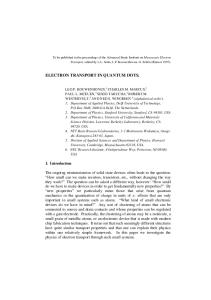
1.3 Photonic crystal waveguides a
Figure 1.2: a, A line defect, i.e.
r
0 .3 4 0 .3 2 0 .3 0 0 .2 8 0 .2 6 0 .2 4 0 .2 2
S la b M o d e s
o d es
F r e q u e n c y [ωa / 2 πc ]
b
R a d ia tio n M
a
S la b M o d e s
0 .3
0 .4 k [ 2 π/ a ]
0 .5
a missing row of holes, in an otherwise perfect lattice of air holes.
The lattice constant is denoted by a, and r stands for the radius of the hole. b, The band diagram of a simple line defect, showing the three propagating modes within the band gap. Typically we work with the fundamental waveguide mode, marked in red.
Photonic crystals are created through a periodic modulation of the refractive index of a material. Bragg scattering at the interfaces leads to the formation of photonic band gaps, akin to electronic band gaps in semiconductors. A nice introduction into this �eld is given in Ref. [12]. In our case the photonic crystals are formed by a periodic array of air holes (n≈
1)
in a GaAs membrane (n≈
3.5).
Removing or shifting holes in an otherwise perfect lattice will lead to the formation of defect states within the band gap. In this thesis we are mostly interested in a particular type of defect called a line defect, see �g. 1.2a. The band diagram of such a structure is shown in �g. 1.2b. Ultimately, we are interested in the interaction between the defect mode and the in-plane transition dipole of a QD and we have therefore only plotted the TE-like modes of the structure. In the black regions there are a continuum of allowed slab guided modes that are not bound to the defect, hence these regions mark
3
Chapter 1. The Basics the edges of the band gap. The green region indicates the light-cone which contains a continuum of leaky modes that are not bound to the slab. The group velocity,
vg , of the waveguide mode is given by
the slope, which goes to zero as we approach the Brillouin zone edge. Thus the group index,
ng = vcg ,
of the mode diverges at the Brillouin zone edge.
1.4 Quantum dots in photonic crystal waveguides Combining the previous two sections we now look at the light-matter coupling between a single quantum dot and the fundamental mode of a photonic crystal waveguide. First we should note that the transition dipoles leading to the x and y-polarized emission are predominantly aligned along the crystallographic directions of the GaAs substrate [13].
Using cleaved edges of the sample as a
reference, the photonic nano-structures can be aligned along the same crystallographic directions. Since the decay rate of the emitter in the waveguide is proportional to the projection of the electric �eld onto the transition dipole moment [14]
Γ ∝ |E(rd ) · d|2 ,
(1.1)
and the waveguide structure is aligned along the same axes as the transition dipoles, it follows that the decay rate of the x and y-polarized transitions are maximized at the extrema of the x and yprojections of the electric �eld, respectively. The ratio between the decay rate of an emitter imbedded in a nano-structure and the decay rate of an emitter in bulk is called the Purcell-factor. In �g. 1.3 a spatial map of the Purcell-factor of the y-polarized dipole (top) and x-polarized dipole (bottom) at
ng = 36
is shown.
For a transition dipole moment optimally aligned with the electric �eld and
positioned at the antinode of the mode-pro�le the Purcell-factor is given by [7]
( PF (ω) =
3λ2 a 4πn3 Ve�
) ng (ω).
(1.2)
7 .0 0 0
+
x y
6 .0 0 0 5 .0 0 0 4 .0 0 0 3 .0 0 0
+
2 .0 0 0
P
1 .0 0 0 0 .0 0 0
F
Figure 1.3: A spatial map of the Purcell-factor, ranging from completely inhibited
cantly enhanced
PF = 7,
PF = 0
to signi�-
for the y-polarized dipole (top) and x-polarized dipole (bottom) at
ng = 36.
The white cross marks one of many spots where both dipoles are enhanced, but to a very di�erent degree. The white cross in �g. 1.3 marks a position where both dipoles are noticeably Purcell enhanced, but to a very di�erent degree. When measuring the decay dynamics of such an emitter the biexponential model mentioned in section 1.2 does no longer apply. Instead, many QDs will exhibit three
4
The β-factor and the importance of specifying the target mode distinct rates, one for each of the two dipoles and one for the decay out of the dark states.
A complete overview of single QDs in photonic crystal nanostructures is given in Ref. [7].
1.5 The β-factor and the importance of specifying the target mode The common thread which connects all chapters throughout this thesis is the
β-factor, and we believe
it to be the most important �gure-of-merit when comparing the performance of 1D-atoms. The factor is de�ned as
β= where and
Γt
Γnr
Γt Γt = , Γt + Γrad + Γnr Γtotal
is the decay rate into the target mode, is the decay rate into non-radiative
Γrad
β-beta (1.3)
is the decay rate into all other radiative modes,
1 modes .
However, if the target mode is not clearly
speci�ed, this can lead to misconceptions about the performance that should be expected for certain applications.
In fact the performance will depend strongly on the optical properties of the actual
emitter used.
In many experiments, including those we present in the next chapter, the target mode is de�ned as the waveguide mode, emission
β-factor.
Γt = Γwg , and we will refer to the β-factor de�ned in this way as the spontaneous
It quanti�es the likelihood that a decay process from the excited state will result
in a single photon in the waveguide mode, but the waveguide mode is spectrally very broad and this value says nothing about the spectral modes of the emitted photons. Thus the spontaneous emission
β-factor
extracted from the decay rates can be thought of as a spatial-mode
β-factor.
However, most
physical phenomena we are interested in, and wish to exploit for the applications discussed in this thesis, rely on interference e�ects between the driving and the scattered �eld. For this interference to take place we require both spatial and spectral overlap of the two �elds. Hence, we should specify a target mode that is single moded with respect to both of these degrees of freedom. For an idealized emitter with only one allowed optical transition from the excited state that can couple to the waveguide, the two ways of specifying the target mode are identical. However, this is not the case for emitters generally used in the experiments.
At this point we want to mention that the
β-factor
and the cooperativity, typically used in cavity
systems, are completely interchangeable as the �gure of merit for our system. The cooperativity is de�ned as
C=
β Γt = , Γtotal − Γt 1−β
and can be extracted in a similar fashion to the spontaneous emission have chosen the
(1.4)
β-factor
2
[15] . The reason we
β-factor as our �gure of merit is because of the rather intuitive interpretation in terms
of mode-selectivity of the scattered light.
1 Most numerical studies of nano-photonic and plasmonic waveguides are interested purely in the radiative β-factor, which assumes an idealized two-level system as the emitter. 2 The de�nition of the cooperativity used here di�ers from that in Ref. [2] by a factor of four.
5
Chapter 1. The Basics In most realistic emitters there exist decay paths that lead to Raman scattering and thus to a �nite probability of the scattered photon being spectrally outside the linewidth of the incident photon. The sum of all the decay rates corresponding to such Raman processes lead to a direct reduction of the
β-factor
into the target mode, relevant for the discussed interference e�ect.
This could either be
due to the non-zero branching ratio for transitions between the excited state and distinct electronic ground-states, as was discussed in the case of the Trion level-scheme shown above, or due to phononsidebands. In the following we give a short phenomenological discussion of the phonon-sidebands in quantum dots and other solid state emitters, but we should mention that similar e�ects should also lead to a reduction of the relevant
β-factor
for schemes exploiting single trapped atoms or ions, when
the experiments do not operate far into the Lamb Dicke regime.
1.5.1 Phonon sideband Several articles investigating the coherent scattering from single quantum dots have shown clear phonon sidebands [16, 17], several nanometer broad and ranging from in the presented data.
5% − 12%
of the total emission
These phonon sidebands have been modeled theoretically and compared to
micro-photoluminescence experiments in Ref. [18]. Following this reference the physical picture used to explain the sideband is that of a formation of exciton-phonon dressed-state level structure.
As
opposed to the dressed state picture in the excited state, the ground state of the system is the neutral QD ground state and a phonon bath. We have illustrated these two manifolds for a particular phonon mode, see �g. 1.4, as two harmonic oscillators where the ladder spacing is given by the phonon energy,
Eq = ~ωq ,
of the mode. Normally the di�erent states in the harmonic oscillator are orthogonal, which
means that the allowed optical transitions would conserve the occupation number of phonons in the system. However, the coupling between the exciton and phonon leads to a shift in the equilibrium position of the lattice [18], shown by the lateral shift of the minima of the excited state parabola in �g. 1.4. This shift leads to a non-zero overlap between states having di�erent phonon occupation numbers and thus to �nite decay probabilities into these states (Franck-Condon principle for lattice vibrations). As shown in �g. 1.4, where the initial state is at T
= 0, interaction with a single phononic
mode leads to several discrete Stokes emission lines when we excite on resonance with the zero-phonon line,
E0 = ~ω0 .
These lines are due to phonon emission and spaced by the phonon energy of the mode
we are considering. Since the exciton can couple to a continuum of phonon modes, the discrete Stokes emission lines turn into a continuous band. At T
> 0,
when there is a �nite initial phonon occupa-
tion, we expect the formation of an anti-Stokes sideband due to phonon absorption, this case is not explicitly shown in �g. 1.4.
The exciton-phonon interaction turns the simple two level system into a multi-level system with additional optical transitions that do not conserve the phonon occupation number, with small but �nite decay rates. The sum of all of these decay processes leads to the formation of sidebands, and thus the integrated intensity of the sideband and the zero-phonon line compared to the total intensity gives the branching ratio of the di�erent decay processes.
When considering the e�ect of the sidebands on the interference discussed above, the simplest case is where we spectrally �lter away everything outside an area corresponding to the zero-phonon line,
6
The β-factor and the importance of specifying the target mode
Figure 1.4: The top and bottom parabolas correspond the excited and the ground state of the quantum
dot and the energy levels within each parabola to the di�erent phonon occupation numbers. At T the population is in the
n=0
ground state. It is brought from the
excited state by a driving �eld resonant with the zero-phonon line,
n=0 E0 .
ground state to the
However, the
n=0
state has a non-zero overlap not only with the corresponding ground state but also with the
n = 2, ...
=0
n=0
excited
n = 1,
ground states. As shown on the far right these transitions lead to Stokes lines in the emission
spectra.
before detection. When doing this, the �nite branching ratio into spectral modes corresponding to the sideband will lead to a direct reduction of the spontaneous emission
β-factor
β-factor.
This is the main di�erence between the
discussed in chapter 2 and the coherent scattering
β-factor
we refer to
in chapter 3 and in chapter 5. One method to minimize this problem would be to move to a di�erent type of QD, with a larger exciton localization length, i.e. larger QDs [18]. Other types of solid state emitters such as single dye molecules embedded in a matrix and NV-centers in diamond have branching ratios into the zero-phonon line which are signi�cantly smaller than those of the QDs discussed here. Typically the zero-phonon line of NV-centers makes up less than 10% of the emission, even at cryogenic temperatures. This rules them out as a candidate emitter for experimental realization of a 1D-atom, unless they are embedded in high-Q cavities designed to selectively enhance the scattering into the zero-phonon line [19]. This illustrates the importance of considering the photonic environment when investigating the e�ect of phonon-sidebands. Following this idea we see that the shape of the LDOS of a standard PCW leads to a strong enhancement of the phonon-sideband for QDs spectrally within a couple of nanometers of the band edge. However, we believe this e�ect can be reduced by engineering the dispersion relation of the waveguide and/or moving to Low-Q, waveguide-coupled cavities far from the waveguide mode band edge.
7
Chapter 2
Spontaneous Emission β-Factor Parts of this chapter are adapted from Ref. [20]. In the previous chapter we discussed possible applications of e�cient single photon (SP) sources in linear optics quantum computing. One approach to achieving high e�ciency SP sources is using a single atom-like emitter coupled e�ciently to a single optical mode. Such a system will additionally enable strong, matter-mediated, photon-photon interaction, which is the essential building block in deterministic optical quantum computation. The basic properties of quantum dots (QDs) and photonic crystal waveguides (PCWs) were introduced, followed by a discussion of the light-matter interaction of QDs embedded in PCWs. Finally we presented the
β-factor
as the �gure-of-merit for such structures. In this chapter a detailed experimental investiga-
tion of the spontaneous emission
β-factor
in PCWs is presented.
Di�erent physical systems have been proposed for obtaining a large rely on the Purcell enhancement thereby increasing
Γwg
suppress the coupling to radiation modes, i.e., decrease an ideal platform to achieve high
β-factors,
β-factor:
plasmonic nanowires
[21], while dielectric nanowires [22, 23] mainly
Γrad .
In this chapter we show that PCWs are
due to the combination of both broadband Purcell en-
hancement into the waveguide mode and a strong suppression of the coupling to radiative loss modes. The preferential emission into a single mode resulting from the combination of these two mechanisms is sketched in �g. 2.1.
It was shown in section 1.4 that the Purcell factor is inversely proportional to the group velocity, and hence diverges when approaching the Brillouin zone edge. In addition to the strong Purcell enhancement into the WG mode, the PC band gap inhibits in-plane decay, while total internal re�ection within the membrane suppresses the out-of-plane decay into radiation modes. A number of theoretical studies have shown that high
β-factors
should be abundant in PCWs [24, 25] and in fact
arbitrarily close to unity can be achieved in theory.
However, measuring a near-unity
experimentally challenging, because the reliable extraction of
Γrad
β-factors
β-factor
is
is not straightforward. Collection
e�ciencies strongly depend on the shape of a given mode in the far-�eld and can vary wildly between di�erent modes. Hence, a direct comparison of the single-photon count rates in the di�erent modes is not a reliable way of extracting spontaneous emission practice to estimate the
β-factor
β-factors.
It has instead become common
by studying the decay dynamics of a QD [26�34]. When measuring
the dynamics the total radiative decay rate of the excited state can be extracted, but it does not
9
Chapter 2. Spontaneous Emission β-Factor allow us to di�erentiate between the radiative decay rates into the di�erent optical modes the QD couples to. It is therefore impossible to separate Experimentally, the waveguide
β-factor
Γwg
in a single decay rate measurement.
and the rate of an uncoupled QD
the case where the di�erence of the total loss rate
β
Γrad
is obtained by recording the decay rate of a QD that is coupled to the
Γc = Γwg + Γrad + Γnr
experimental
and
is written as
β=
Γrad + Γnr
Γuc = Γrad + Γnr .
This is valid in
between the two QDs is negligible. The
Γwg Γc − Γuc . = Γwg + Γrad + Γnr Γc
(2.1)
This approach has been used in a number of studies and we start by summarizing the literature, discussing their results and experimental methods.
The understanding gained from earlier work is
used in the design of new waveguide samples and new experimental methods and setups.
2.1 Summary of previous work Di�erent attempts of measuring the
β-factor
in photonic-crystal waveguides have been published,
but despite the theoretical predictions the highest value of the
β = 89%.
This value was measured by Lund-Hansen
et al.
β-factor
reported in the literature is
[26] using a top-collection confocal setup.
In such a setup both excitation and collection of the QD emission are done from out-of-plane of the WG mode and at the same spot on the sample.
Simply due to the geometry of the measurement
this method preferentially probes QDs with relatively low coupling e�ciency, since high decay into radiative loss modes very weakly, see �g. 2.1.
β-factor QDs
Additionally the propagation loss in our
structures is low leading to well coupled QDs becoming essentially undetectable in out-of-plane measurements. Furthermore, it is challenging to properly determine the decay rate of an uncoupled QD by this method, since the spatial resolution of the collection optics is not su�ciently high to ensure that all detected lines originate from QDs spatially positioned in the waveguide. Indeed a proper measurement of the
β-factor requires the precise determination of Γuc = Γrad + Γnr ,
where
Γrad
is the rate
of coupling to the radiation modes for a QD that is spatially positioned within the waveguide mode as opposed to in a defect-free region of the PC membrane. In fact detailed �nite element frequency domain (FEFD) simulations show that estimating the loss rate by measuring in a defect free region of the PC can lead to underestimates of
Γrad
[7].
In order to overcome the potential issue of spatial mismatch, one approach has been to tune a Purcell-enhanced QD across the waveguide band edge and into the band-gap region [27]. By choosing a Purcell-enhanced QD one can guarantee that the emitter is spatially positioned within the WG mode. However, one has to keep in mind that tuning quantum dots spectrally over several nanometers, either by magnetic �elds, electric �elds or by temperature tuning, is likely to alter their intrinsic properties. These tuning mechanisms can change the polarization of the transition dipole moment, the oscillator strength, and the non-radiative decay rate.
The approach of temperature tuning is limited by the
rather elevated temperatures required to obtain a su�ciently large tuning range (10 cause an increase in the nonradiative decay,
Γnr ,
− 60K),
which
and residual coupling to the waveguide mode due to
phonon-mediated processes. Such phonon-mediated coupling has been observed for PC cavities [35] and similar broadband e�ects are expected when tuning into the band-gap below the waveguide cut-
10
Summary of previous work
G
r a d
G
Figure 2.1: Illustration of the device.
w g
A train of single-photon pulses (red pulses) are emitted from
a triggered QD (yellow trapezoid). The photons are channeled with near-unity probability into the waveguide mode with a rate
Γwg
while the rate
Γrad
of coupling to radiation modes is very weak
and thus only very few photons are lost. The guided photons can be e�ciently extracted from the waveguide through, for example, a tapered mode adapter.
o�. Both of these e�ects signi�cantly contribute to
Γuc ,
and thus limited the extracted values of
β
to
85.4%. Additionally in both of these approaches it was assumed that the radiative loss rate is frequency independent, which in the worst case can lead to systematic overestimates of the
β-factor
[25].
In recent work, experimental e�orts have shifted towards the direct collection of photons coupled to the waveguide mode [32, 33, 36]. However,
Γuc
was still extracted in a top-collection scheme [32, 36],
either from QDs sitting in a defect-free PC or with a method similar to that used in Ref. [26]. These approaches have the drawback of neglecting the changes of the coupling to the radiation modes due to the presence of the line defect. In addition Ref. [33] did not take into account any variation of
Γnr
between di�erent QD samples used in di�erent experiments.
In this chapter we discuss our measurements performed in the side collection geometry, where the
β-factor mode
Γc
is experimentally determined by comparing the decay rate of a QD coupled to the waveguide to that of a very weakly coupled QD, which constitutes an upper bound of
the key di�erences to previous work is that both
Γc
and
Γuc
Γuc .
One of
are obtained by directly detecting the
propagating waveguide mode, hence all measured QDs are spatially positioned in the waveguide. This guarantees that the spatial and spectral dependence of the coupling to radiation modes due to the presence of the PCW can be taken correctly into account, which is essential for the analysis.
The
majority of measurements presented in this thesis were done in side collection and in the following sections we discuss the sample designs and experimental setups that were necessary to perform these measurements.
11
Chapter 2. Spontaneous Emission β-Factor
2.2 Side collection samples With the term "side collection" we refer to all experiments where the measurements are performed directly on the propagating waveguide mode. E�cient out-coupling of the propagating mode is essential for such measurements, and two types of mode adapters were used. Both of these mode adapters transform the in-plane waveguide mode to a well de�ned free-space mode, which can be collected using standard bulk optics. We have previously shown that the light-matter coupling for a QD in a PCW is expected to be the strongest when the mode approaches the Brillouin zone edge where the Purcell factor diverges because it is inversely proportional to the group velocity. Coupling extremely high group index modes to freely propagating modes poses a technical problem which will have to be overcome in these samples. The �rst mode adapter is a second-order grating, designed to couple the in-plane propagating mode orthogonally out-of-plane [37]. This type of grating is well established for out-of-plane butt-coupling from �ber to in plane waveguides [38, 39] and has also been used in the design of photonic bullseye structures [40]. The second mode adapter is an inverse tapered mode adapter [41] where the working principle is equivalent to that used to demonstrate highly e�cient outcoupling from semiconductor nanowires [22, 42] and silicon-on-insulator waveguides [43].
However,
both of these mode adapters work best in the low-ng region of the waveguide mode while the high-ng region is well suited for coupling to QDs. To optimize the performance of the mode adapters we �rst couple the slowly propagating mode into a slightly altered PCW that supports a mode propagating at a higher group velocity for the same frequency. Even for very high-ng modes the coupling to the low-ng waveguide can be facilitated by a short transition region, only few lattice constants long [44]. To minimize the overhead involved with doing detailed numerical studies to optimize the out-couplers we took advantage of the scale-invariance of Maxwell's equations and adapted designs from the literature for our desired wavelength range. More recently however, detailed numerical studies of the fabricated samples have been performed in our group and optimization is being done for the second generation of out-coupling mode adapters.
2.2.1 Second-order grating out-coupler To give a simpli�ed explanation of the operational principles of the grating we start by considering a single in-plane propagating mode with wavevector pointing in the
x-direction |kx | =
2πn λ0
=
2π λ . As
opposed to standard Bragg re�ectors, which are designed so that the wavevector corresponding to the periodic modulation of the grating period of modulation is
Λ = λ/2),
|K| =
2π Λ is twice the wavevector
kx
of the incident light (i.e. a
the grating mode adapter is designed with a total period
Λ = λ.
Conservation of energy and of momentum has to be ful�lled when scattering at these two di�erent types of gratings and is to �rst order given by
kin = kout + K.
(2.2)
ωin = ωout .
(2.3)
While in a standard Bragg re�ector the quasi-momentum contributed by the grating leads to the �rst-order scattering process
kx → −kx ,
maps the in-plane wavevector to zero,
the �rst order scattering process in the second-order grating
kx → 0,
�g. 2.2a. This leads to scattering into the direction
orthogonal to the incoming wave, where the out-of-plane wavevector is given by
12
ky = y ˆ ωout c .
The
Side collection samples designs used are based on the work in Refs. [37, 45], where the above idea is extended to 2D, and is shown in �g. 2.2b. Most of the structures were designed to have a
50% duty-cycle,
which is de�ned as
the ratio between the optical path length in the material and the total optical path length for a single period of the grating. The far-�eld calculated from FEFD simulations of the grating out-coupler are shown in the insets of �g. 2.2c. is found to be
= 0.82
NA
≈ 45%
and
, respectively.
The collection e�ciency of the grating far-�eld into the �rst lens
≈ 70%
for numerical apertures NA
= 0.65,
used in the experiment, and
These calculations were performed for a dipole source emitting into the
high-ng region of the waveguide which is coupled into the low-ng before reaching the out-coupler, and this transition region will be discussed in section 2.2.3. This e�ciency has to be divided by two due to
a
B r a g g r e f le c t o r K
S e c o n d - o r d e r g r a t in g k
k
b x
1 µm
x
2
2 n
Λ
K
c 7 0 %
N A = 0 .8 2
5 0 %
N A = 0 .6 5
G r a t in g E f f ic ie n c y
6 0 % 4 0 %
d lE l2
3 0 %
1 .0
2 0 %
0 ,5
lE l2
0 .5 0 .0
1 0 %
0 %
e
8 9 0
9 0 0
1 ,0
9 1 0
W a v e le n g t h ( n m )
9 2 0
0 ,0
-1 ,0
-0 ,5
0 ,0
N o r m a liz e d R a d iu s
0 ,5
1 ,0
Figure 2.2: a, Illustration of the basic operating principle of the second order grating. For a standard
Bragg re�ector the wavevector of the crystal momentum in-plane propagating mode
K.
kx
K
is twice as large as the wavevector of the
at the design frequency is exactly canceled by the crystal momentum
Hence, the mode is scattered out-of-plane. b, SEM image of an out-coupling grating similar to
the ones used in measurements. c, Collection e�ciency of NA coupler far-�eld at two di�erent wavelengths with NA
= 0.65
= 0.65
lens. Insets: The grating out-
indicated by the black dotted line. d,
The di�erent cross sections of the far-�eld indicate by the light blue, dark blue, red and brown lines in the insets of c, respectively. e, Three alternate designs of out coupling gratings are shown here.
13
Chapter 2. Spontaneous Emission β-Factor the up-down symmetry of the out-coupler (ignoring re�ections from the substrate) and another factor of two, since the structures used in this thesis are mostly designed for transmission experiments and therefore out-coupled on both sides. Leading to a �nal collection e�ciency of
≈ 11%
of the emission
that couples to the waveguide mode. Additionally, we can see from the insets in �g. 2.2c and from �g. 2.2d that the far-�elds are non-gaussian and will thus have a poor overlap with the mode of a single-mode �ber leading to additional losses at the �ber-coupling.
A large number of additional
grating designes have been fabricated. Mainly on passive wafers to test their structural stability. The number of grating periods, the grating support beams, as well as the duty cycle of the grating were varied.
2.2.2 Tapered out-coupler In the tapered out-couplers an adiabatic transition from the waveguide mode to the free-space propagating mode is implemented. As the width of the taper decreases the mode becomes more and more delocalized from the high-index material adiabatically reducing the e�ective refractive index and hence avoiding back-re�ections that would occur at an abrupt GaAs-to-air interface. Additionally, the mode �eld diameter is gradually increasing as the e�ective refractive index is reduced, thus reducing the divergence angle of the free-space mode [42]. This has been successfully demonstrated for GaAs-based PCWs operating at Telecom-wavelengths [41], and this design has been adapted for our wavelengths. The tapper length is scaled with the lattice constant of the PCW,
L = 6a.
An SEM image of a
fabricated taper is shown in �g. 2.3a. The collection e�ciency into the �rst lens for the inverse-taper far-�eld is found to be very similar to that of the grating coupler, numerical apertures NA
= 0.65
and NA
= 0.82
≈ 45% − 50%
and
≈ 70%
for
, respectively. In the majority of the structures both
sides of the waveguide are terminated by out-couplers and we have to divide the e�ciency by a factor of two to get the �nal collection e�ciency into the �rst lens, of
≈ 23%,
for a photon emitted into the
waveguide mode. From the insets of �g. 2.3b and from �g. 2.3c we can see that the far-�eld of this mode-adapter has a larger overlap with the �ber mode, since its shape is signi�cantly more gaussian than those of the second-order grating coupler.
2.2.3
Fast-to-slow transition
As is mentioned above both of these out-couplers work best in the fast-light regime (low-ng mode), while light-matter interaction is stronger in the slow-light regime (high-ng mode). This problem is solved by having two di�erent waveguide regions in each PCW, see �g. 2.4a. The band structure of the two regions is shown in �g. 2.4b where it is clearly seen that the red waveguide band has a region of low-ng modes overlapping with the region of high-ng modes of the blue waveguide band. Intuitively one would think that the re�ection coe�cient at such an interface scales as the standard Fresnel coe�cient, and there will be signi�cant re�ection when coupling two modes of di�erent
ng .
This can
be argued by considering the two waveguides as two di�erent e�ective media and the Poynting vector across such an interface [46].
While the direction of the Poynting vector gives the direction of the
energy �ow, its magnitude is given by the intensity
14
I = uvg ,
where
u
denotes the energy density and
Side collection samples a b
7 0 % 6 0 %
N A = 0 .8 2
N A = 0 .6 5
5 0 % 4 0 %
lE l2
3 0 %
6 a
1 .0
2 0 %
0 .5
0 .0
1 0 %
0 %
c
1 µm
Figure 2.3:
8 9 0
1 ,0
9 0 0
9 1 0
9 2 0
W a v e le n g t h ( n m )
lE l2
0 ,5 0 ,0
-1 ,0
-0 ,5
0 ,0
N o r m a liz e d R a d iu s
0 ,5
1 ,0
a, SEM image of a tapered out-coupler similar to the ones used in measurements.
Collection e�ciency of a NA
= 0.65
and a NA
far-�eld at two di�erent wavelengths with NA
= 0.82
= 0.65
.
b,
Insets: The inverse tapered out-coupler
indicated by the black dotted line. c, The cross
sections of the far-�eld indicate by the respective colours in the insets of d.
vg
1
is the group velocity of the mode . The energy density is given by
u= where
ϵ
is the absolute permittivity,
µ0
B2 1 (ϵE 2 + ), 2 µ0
is the vacuum permeability, and
E
and
B
are the electric
and the magnetic �elds. Looking at the dashed line in �g. 2.4a, which marks the transition between the two waveguide sections, we can see that the absolute permittivity is continuous across this line and hence the �eld is continuous across the doted line. Therefore, the energy density on both sides of the line should also be continuous, but the group velocities in the two sections are very di�erent leading to drastically di�erent magnitudes of the Poynting vectors in the two PCW sections, when considered independently. Since we can not have a pileup of energy at the boundary there must be a signi�cant re�ection in the transition region. This argument ignores the transverse pro�le of the mode and implicitly assumes that the two Bloch modes propagating at di�erent speeds have similar shapes. While this almost holds for PCWs in a square PC lattice this is not the case for PCWs in a hexagonal PC lattice [44, 46]. A detailed explanation of how evanescent Bloch modes in the transition region aid in the coupling in the case of a hexagonal lattice is given in Ref. [46]. This decreased impedance mismatch between di�erent group velocity modes in hexagonal lattice PCWs can be exploited and low-ng modes are used as e�cient injectors into high-ng modes. We create the low-ng (red) waveguide by stretching the lattice in the
y-direction.
450 x-direction, a′ = a 420 , while keeping the lattice spacing constant in the
Hence, we also sometimes refer to the red waveguide as the stretched lattice waveguide.
Additional small changes to the periodicity of the lattice right at the transition between the two WGs
1 This
relation between I , u, and vg assumes that we can treat the PCWs as an e�ective homogeneous medium and does not hold for periodic structures. In PCWs we should replace u by the average energy density over one unit-cell to obtain the correct value of vg [12].
15
Chapter 2. Spontaneous Emission β-Factor can be used to create a coupling region which increases the injection e�ciency [44]. The transition region of the samples designed for this thesis were used with either no coupling region or a coupling region designed for the transition
ng = 100
a
to
ng = 5 . b
F a s t S lo w
F r e q u e n c y [ ωa / 2 πc ]
0 ,2 8
0 ,2 6
F a st
S lo w
0 ,3
F a st
ng
Figure 2.4: a, SEM image of a high-
k x
0 ,4
[ 2 π/ a , 2 π/ a ' ]
0 ,5
region (blue) and two low-ng regions on either side (red). In
the red waveguide the lattice constant in the propagation direction
a′
is stretched by
450 420 , while the
lattice remains unchanged in the direction orthogonal to the propagation direction. The additional rows of holes on the side of the PCW are used in experiments to identify the region of the structure containing the blue mode waveguide. b, The even waveguide bands for the two PCW sections are plotted for the same frequency axes, the frequency range interesting for application is marked in grey. These bands were calculated for a membrane thickness of
h=
16 26 a and a �lling ratio of
r/a = 0.3.
2.3 Side collection setups In the following we introduce the two setups that were used for the experiments discussed in this chapter.
To overcome non-radiative recombination, minimize the e�ect of phonon-dephasing, and
reduce the amount of emission in the phonon sidebands these experiments have to be performed at cryogenic temperatures.
All the experiments we discuss have been performed at temperatures
between 4 and 10 K, and the cryostats used to facilitate these types of measurements are described below. In order to investigate both the spectral properties and the decay dynamics of the QD samples we �rst create an excitation in the QDs. For spectral studies the sample is excited by an above-band continuous wave (CW) excitation laser.
A number of lasers like the Helium-Neon gas lasers and a
Titanium Sapphire laser operated in CW-mode are available for these measurement. For high QDdensity samples taking spectra at excitation powers above single-QD saturation is used as the �rst characterization step, this takes advantage of the inhomogeneous broadening of the QDs to obtain information about the density of optical states (DOS) of the photonic structure. On the other hand, time-resolved studies of QDs give us information about their local photonic environment, i.e. their local density of optical states (LDOS). For time resolved measurements a pulsed excitation source is
16
Side collection setups necessary and the same titanium-sapphire laser (Coherent Mira 900) can be used as a mode-locked laser, able to operate in pico-second and femto-second mode.
Figure 2.5:
This schematic shows the optical paths on the laser table.
We have only included the
sources used in this part of the thesis. The combination HWP and PBS right at the Mira output, labeled by 1 and 2, are used to split the output power into three arms. Two of these arms are coupled into PM-�bers that bring the laser to the cryostats, while the third is sent on the TDA200 photo diode (PD) used to generate the sync signal for time correlation measurements. Each of the three arms has an additional HWP and PBS to control the power in the arm. The beam splitters BS1 and BS2 are are part of a variable delay arm which can be used for HongOuMandel-measurements, but was not used during this thesis. A mirror on a magnetic mount (MM) can be inserted into arm 1 when the variable repetition rate pulsed laser diode (PLD) is used.
The Ti:Sapphire is pumped by a solid state laser which generates up to and can produce close to
2
in pico-second mode (∼
ps). These pulses are su�ciently short compared to typical QD dynamics to
3
W at
800
10 W at 532 nm (Verdi G10)
nm. For our measurements the Ti:Sapphire is usually operated
be viewed as delta-function like excitation. Pico-second pulsed lasers are preferable to those operated in femto-second mode since the spectral width of femto-second pulses can lead to problems when moving to quasi-resonant excitation. The laser has a repetition rate of separation of
∼ 13
ns.
76 MHz corresponding to pulse
For the measurement of slow decay rates, where the lifetime of the excited
state becomes comparable to, or longer than, the pulse separation, the emitter will not be able to fully decay between excitation events leading to unwanted saturation e�ects. Therefore, we instead use a pulsed laser diode emitting at a pulse separation of up to
∼ 785
200
nm with a variable repetition rate of
80
MHz to
5
MHz, giving
ns. The two pulsed lasers can be coupled into the same single-mode
polarization-maintaining (PM) �ber on the laser table (�g. 2.5) and we can easily switch between the two using a mirror mounted on magnetic base plate. There is a second beam path split o� from the Mira output, also coupled into a PM �ber, which allows the laser table to be shared between multiple
17
Chapter 2. Spontaneous Emission β-Factor setups. Before either of the PM �bers a half-wave plate (HWP) in combination with a polarizing beam splitter (PBS) is used as a variable power control. A third beam path is taken from the Mira output and sent to a fast photodiode(TDA200). This diode generates a sync signal for the time correlation measurements used to study the decay dynamics of the QDs.
Figure 2.6:
This schematic shows the optical paths on the table we use for spectral analysis.
The
emission is brought from the cryostat via PM-�ber and the axis of the �ber is aligned with the polarization corresponding to the highest grating e�ciency. A mirror can be inserted into the beam path right after the �ber out-coupler via a �ip mount to direct the light to a Fabry-Perot interferoemter (FPI), otherwise the beam is directed to the spectrometer.
The exit mirror in the spectrometer is
�ipped out of the path for spectral studies of the emission and �ipped into the path for investigation of the decay dynamics of QDs and for autocorrelation measurements. The BS after the spectrometer is sitting on a magnetic mount, allowing us to remove it when measuring decay dynamics of single quantum dots since it is only needed for autocorrelation measurements.
Spectral analysis of the emission from the sample is done using the SP-2558 from Acton Research Corporation which can be used either as a spectrograph or as a monochromator depending on the exit mirror position, which selects between the two output ports (�g. 2.6). When used as a spectrograph the exit mirror is �ipped out and a line of spectral components impinge on a thermoelectrically cooled CCD array made up of
1340
by
100
pixels (Pixis100).
For time resolved measurements the
exit mirror in �g. 2.6 is �ipped in and the spectrometer functions as a monochromator, where a single spectral component exits through the output slit. After the monochromator the light is focused onto a single photon avalanche photodiode (APD) with a detection e�ciency of and a timing resolution of roughly
250
ps for a correctly focused beam.
∼ 35%
at
920
nm
The output port of the
APD is connected to a time tagging module (PicoHarp300) which assigns an individual time tag to each incoming photon count with up to
18
4
ps timing resolution.
Alternatively the PicoHarp300
Side collection setups can be used as a time-correlated single photon counting module. In this mode the individual time tags are not recorded, instead a time-correlation histogram between the excitation pulse (sync signal from the TDA200 trigger diode) and the single-photon detection events are accumulated. In addition to the spectrometer we have a grating setup (not shown here) where the output goes directly into �ber coupled APDs, which can be used when higher system throughput is necessary. This becomes important when performing correlation measurements. Ref. [47]. Inserting a
50 : 50
More details on this setup can be found in
beam splitter together with an additional APD (see �g. 2.7) allows us to
do autocorrelation measurements on the spectral component transmitted through the monochromator.
While there are very speci�c requirements to the setup for measurements on the samples terminated by the inverse taper mode adapter, due to the orthogonality of excitation and collection beams, those terminated by gratings can be used in rather standard experimental setups. These two types of outcouplers are mainly used in a customized helium bath cryostat and a standard helium �ow cryostat respectively, and the two setups are described in the following.
2.3.1 Bath cryo The helium bath cryostat used is an ATTOLIQUID1000 (attocube) with a customized cfm-2 microscope insert, �g. 2.7a. This insert was designed to accommodate measurements on the inverse taper terminated PCWs. The insert tube is partially submerged in the liquid helium bath, which keeps the sample at a constant temperature of
4.2
K. Pumping on the liquid helium reservoir with a vacuum
pump can further reduce the temperature to
∼2
K. The sample stick is not in direct thermal contact
with the insert tube and the sample is cooled via an exchange gas (20 sample can be imaged by two orthogonal objectives, the �rst (NA=
30
mBar of helium gas). The
0.65)
coupling to a free space
beam that is out-coupled vertically from the cryostat dewar, is used for collection, while the second (NA=
0.5)
is SM-�ber coupled and oriented orthogonal to the �rst one. This objective is used for
excitation, �g. 2.7b. The �ber coupled objective and the sample are each mounted on their respective three-axis piezoelectric nano-positioners (ANPxyz51), which allow us to position them with respect to each other and the free space objective. Between the stages and the sample there is a heater allowing us to heat the sample. A minimum step sizes of of
2.5
mm
× 2.5
10
nm is achievable at
4
K for a total travel range
mm. As shown in �g. 2.7c the sample is mounted vertically with the taper pointing
directly towards the free space objective. Additionally, each of the three axis-positioners is equipped with a scanning-piezo allowing us to do confocal re�ection imaging with the �ber coupled objective, �g. 2.7b. Both of the objectives are monochromatic lenses, since composite lens systems required for achromatic objectives usually depend on the use of optical glues, which quickly degrade at cryogenic temperatures. This forces most of the alignment to be done with laser diodes close to the emission wavelength.
A high-NA, achromatic objective made completely without optical glues (NA=
0.82)
has been bought and will be used in future experiments. Illumination of the sample, which greatly simpli�es the positioning of the stages, is done by an LED emitting at
850
nm and the scattered
light is imaged by a CCD camera. These components were originally added to the microscope head delivered by attocube, but due to mechanical stability issues of the delivered product this has been replaced by a much more stable breadboard solution, �g. 2.8a. The breadboard is directly mounted on the dewar and therefore o�ers the same isolation from outside vibrations as the microscope head,
19
Chapter 2. Spontaneous Emission β-Factor
a
c
b
Figure 2.7:
a, Cross section of the helium bath cryostat.
springs in order to damp vibrations from the outside.
The dewar is hanging from its frame by
A SM-�ber brings the excitation laser from
the laser table and enters the cryostat through an optical �ber feedthrough all the way to the sample sitting at
∼4
K. The sample is mounted at the very bottom of the sample stick which sits inside the
insert tube. The superconducting (SC) magnet surrounds the bottom of the insert tube. The emission is polarization �ltered and coupled into PM-�bers on the breadboard mounted on top of the dewar. b, A zoom in to the bottom of the sample stick showing the orthogonal objective excitation-collection
setup needed to measure on the inverse tapered samples. Both the excitation objective and the sample are mounted on three axis nano-positioner stacks in order to align them with respect to the collection objective. c, Illustration of the sample, emission is shown in red and the above band excitation laser is shown in green. The cone of light labeled emission is pointing towards the collection objective.
but greatly improved the mechanical stability. This made the collection less sensitive when optimizing the alignment and created space for additional optics on the cryostat, needed for further optimization of the setup.
The above-band excitation laser is coupled into the SM-�ber leading to the �ber coupled objective. The excitation laser spot can then be moved along the waveguide structure in the search for a suitable QD using the nano-positioners, while keeping the collection �xed. The waveguide emission is polarization �ltered by the combination of a quarter-wave plate (QWP), a HWP, and a linear polarizer (LP) �xed to the optical axis of the PM-�ber used in collection. The axis of the PM-�ber output is aligned on the detection setup �g. 2.6 so it agrees with the polarization that gives the highest grating e�ciency in the spectrometer. Rotating the HWP before the LP we can switch between collecting the
20
Side collection setups b a
2 5 0
T M
2 0 0
T E
C o u n ts/s
1 5 0 1 0 0 5 0 0
Figure 2.8:
8 8 0
9 0 0
9 2 0
9 4 0
W a v e le n g t h [ n m ]
9 6 0
a, Top view of the breadboard setup that has replaced the standard microscope head.
There is a hole in the middle of the breadboard through which we access the cryostat window. The combination of QWP, HWP and LP used for the polarization �ltering is between the cryostat window and the breadboard and not shown here. b, Two spectra taken under identical excitation conditions for two orthogonal settings of the polarization �lter to distinguish between the TE and TM modes(WG design parameters:=
242, r/a = 0.27).
The black dashed line indicates the edge of the blue PCW
mode. Inset: Schematic shows where the sample is excited (green spot) and from where the emission is collected (red cone).
We are exciting in the red waveguide section, but are only collecting the
emission that has been �ltered by the mode in the blue waveguide section.
TE-mode and TM-mode of the PC-membrane. Initial measurements were performed on PCWs with inverse taper out-couplers at liquid nitrogen temperatures and strong above band excitation �g. 2.8b. The excitation laser was placed in the low-ng waveguide section (red mode) away from the taper out-coupler. On the way to the taper the QD emission passes the high-ng waveguide section (blue mode) which behaves like a spectral �lter only passing the section of the red WG mode that overlaps with the blue WG mode in �g. 2.4b. In the spectral region where the red and blue modes overlap we see that all the emission stays in the TE-mode and very little polarization mixing is observed when propagating through the sample. While the frequency range below the cut-o� of the blue mode (black dashed line in �g. 2.8b) shows signi�cant scattering into TM-modes.
Finally, there are also
small features of TE polarization close to the cut-o� of the red mode, seen on the right of �g. 2.8b. We believe this occurs because the band-edge of the mode in the red section, right at the cut-o�, is spectrally outside the band gap of the blue section and can therefore couple to slab modes.
During the course of this work the setup was extended to include a
9
T super-conducting magnet,
and initial tests both in Faraday and in Voigt geometry have been performed, showing the typical behaviour as a function of magnetic �eld outlined in Ref. [8].
More detailed studies involving the
magnet are planned in future low QD-density samples. Finally, one of the main bene�ts of the bath cryostat is its long term stability, enabling uninterrupted data collection over several days.
21
Chapter 2. Spontaneous Emission β-Factor
2.3.2 Flow Cryo
Figure 2.9: A PM-�ber brings the excitation laser from the laser table. After the �ber a HWP and
a PBS are used to set the power on the sample and a 50:50 BS is used together with a powermeter (PM) to monitor the power sent to the cryostat. An additional HWP after the BS is used to set the polarization incident on the sample. The two mirrors marked by dashed squares in the microscope can be taken in and out of the setup depending on if the white-light source and the CCD are being used or not. The �nal HWP and PBS pair is used to switch between collection of TE and TM. Inset: A waveguide terminated by a grating at each end is excited by an above band laser (dim spot in the middle) and emission is seen out of each of the gratings (bright spots). Image is taken by the CCD after passing through the dichroic mirror (BSP/DM) which suppresses the scattered laser light.
The helium �ow cryostat is the MicrostatHires2 from Oxford Instruments. The setup around this cryostat is easily adapted for a large number of applications ranging from simple QD characterization to resonant QD experiments. In the Hires2 the sample sits on a stable cold platform which is in direct contact with the heat exchanger. The heat exchanger is cooled by a �ow of liquid helium supplied through the transfer tube. Special precautions are taken in the design of the thermal connection from liquid helium �ow to the sample holder to minimize the amount of vibrations on the sample. These vibrations are typically kept below
20
nm, which is essential for the study of single QDs in photonic
nanostructures. The cryostat is mounted on two translation stages allowing us to position the sample with roughly
100
nm precision with respect to the objective. These stages allow large area scanning
of the sample, which is very convenient for initial characterization. However, the stages are not very stable to external pressure on the cryostat and the e�ect of tension on the transfer tube is one of the main causes of instability in the setup (�g. 2.9).
A microscope is permanently mounted above
the cryostat (Olympus BXFM) and has two beam-paths, one for excitation and one for collection. The objective used in the microscope (NA=
0.6
from Nikon) was chosen because it can compensate
for the aberrations caused by the cryostat window (∼
22
1.5
mm of crystalline quartz). The excitation
Side collection setups laser is brought to the table by a PM-�ber, which assures a constant polarization. The beam passes through a HWP and a PBS, used to control the power. Half of the remaining power is split o� at the BS and sent to a powermeter, to give a reference for the power that is sent to the sample. The last optical component before the microscope objective is mounted on a �lterwheel and can easily be switch between a standard 90:10 beam sampler (BSP), used when imaging the sample on the CCD while illuminating with the white light source, and a dichroic mirror used for imaging the emission and when taking measurements. The dichroic mirror re�ects below
875 nm and transmits above it, serving
as the �rst step of the spectral �ltering when measuring QD emission under above-band excitation. The two mirrors surrounded by dashed lines can be moved in and out of the beam path depending on if we want to image the sample on the CCD or send the emission to the detection PM-�ber. Before the PM-�ber that is used in detection there is another HWP followed by a PBS which is used to polarization �lter the emission before coupling to the detection �ber. Since the grating out-coupler maps TE- and TM-polarization to di�erent far �eld polarizations, the HWP and PBS can be used to
0 ,8
0 ,8 0 ,6
In t e n s it y
0 ,6 B a n d g a p
F P fr in g e s
0 ,4 0 ,2 0 ,0
H IG H P O W E R
1 ,0
8 9 5
9 1 5
W a v e le n g t h (n m )
B a n d g a p
b
H IG H P O W E R
1 ,0
In t e n s it y
a
W G m o d e
distinguish the TE-mode from the TM-mode.
0 ,4 0 ,2 0 ,0
9 3 5
8 9 0
9 0 5
9 2 0
W a v e le n g t h (n m )
9 3 5
Figure 2.10: High power spectra taken to illustrate the DOS of the investigated waveguide structures.
a, A waveguide terminated by a PC on one side and by a grating on the other side exhibits strong
FP resonances. For this measurement the excitation laser spot was in the red section of the structure (WG design parameters:a
= 238, r/a = 0.25).
b, A waveguide terminated by a grating on either side.
The DOS is more like that expected for a waveguide, with a strong increase towards the band edge. As shown in the schematic the excitation spot was positioned on the blue section of the waveguide (WG design parameters:a
= 238, r/a = 0.25).
This cryostat was only used for the samples terminated with the grating out-couplers. The two types of structures used and their respective emission spectra under high power (far above single QD saturation) excitation are shown in �g. 2.10a and b. Fabry-Perot (FP) resonances.
The results shown in �g. 2.10a show strong
The free spectral range (∆FSR ) between neighbouring resonances is
given by
∆FSR,λ = where
Lng (λ) = Lopt (λ)
λ2 2Lng (λ)
(2.4)
is the optical path length in the resonator, which is dispersive. This allows
us to extract the wavelength dependent group index of the fabricated samples, which is used for the
23
Chapter 2. Spontaneous Emission β-Factor simulations presented together with the measurements in section 2.4. How accurately we can extract
ng
is mainly given by the physical length of our sample, since this determines the
how large a wavelength range we average over for each extracted
ng .
∆FSR
and thus
The strong resonances shown
in �g. 2.10a are seen because one side of the sample is terminated by photonic crystal causing almost perfect re�ection.
Additionally, slightly di�erent gratings were fabricated for the sample used to
extract the group index. The grating duty cycle was changed and the total grating period increased. Similar changes to the grating showed an increase in re�ectivity in numerical simulations. A more detailed discussion and additional measurements are given in [47].
2.4 Measurements of β-factor Using the tools described above in section 2.2 and section 2.3 we are ready to start systematic measurements of the
β-factor
in side collection. The most natural place to look for well coupled QD is
close to the band edge of the PCW mode, where we expect strong Purcell enhancement. However, we now face the problem of avoiding e�ects of Anderson localization present due to intrinsic fabrication disorder in photonic crystal membranes [48]. Interaction with an Anderson localized mode can lead to cavity enhanced decay rates and therefore leads to incorrect extraction of the mode. The e�ective
β-factor
β-factor
into the PCW
of such a cavity-waveguide system includes the coupling e�ciency of the
cavity to the waveguide mode, and since we observe strong out-of-plane emission from many of these cavity modes we know this coupling e�ciency to be low in general. In order to avoid this problem we take special care to measure on QD lines spatially and/or spectrally displaced from Anderson localized modes, the location of which are identi�ed in high-power spectra.
The second problem is related to the extraction of the decay rate of an uncoupled transition,
Γuc ,
Γuc
has
close to the waveguide mode band edge. As we mentioned above the correct extraction of
been one of the limiting problems in experimentally con�rming the theoretically predicted near-unity
β-factors
[24, 25]. Although we have ruled out the issue of measuring QDs spatially and spectrally
outside the waveguide mode by moving to side collection experiments, we encounter the problem of �nding a QD that is weakly coupled to the mode. From simulations (see for example �g. 2.12b) we expect that even close to the band edge there are many positions in the mode where one of the two dipoles is weakly coupled, but since both of the orthogonal dipoles project onto the same waveguide mode we have no means of polarization �ltering between the orthogonal dipoles and our measurements always include all the di�erent rates described in section 1.4. Due to the relatively large density of QDs in the sample the extraction of the slower components when �tting the data can be in�uenced by other transitions decaying into the same spectral window even when no other clear QD emission lines are in the proximity [49]. Therefore, taking the slower decay rates �tted with our double and triple exponential models as the uncoupled rates is not a good approximation. we discuss two approaches to measuring the uncuopled rate,
Γuc ,
In the following sections
and thus the
β-factor.
To show
the validity of our method a detailed comparison between experiments and numerical simulations is necessary. However, since the theoretical Purcell-factor diverges as we approach the Brillouin zone edge it is important that we limit the simulations to experimentally realistic values of the group index.
We independently determined the range of realistic group indexes by measuring on structures like
24
Measurements of β-factor the one shown in �g. 2.10a. In �g. 2.11a a scanning electron microscope (SEM) image of a sample that can be used to extract the dispersion relation of the waveguide mode is shown. As discussed above, these waveguides are terminated by a photonic crystal on one side and by a grating mode adapter on the other side. While the waveguides have the same design parameters as the samples where the
β-factors
have been measured, the grating is designed for longer wavelengths and has a di�erent duty
cycle than the gratings used in
β-factor measurements leading to an increased re�ection back into the
waveguide. The band edge of the blue (red) waveguide mode is spectrally positioned at around
930
nm (960 nm). The measurements are performed by moving the excitation spot along the waveguide from the blue to the red section in �g. 2.11a, and collecting the photoluminescence from the grating.
a
c 1 0 0
E x p n E x p n
lS 1 ,0 5
In t e n s it y
0 ,8 0 ,6
0 ,0
Figure 2.11:
1
2
1 7
2 3
5 6
9 2 0
( λ) 7
9 3 0
9 4 0
6
W a v e le n g t h ( n m )
2
7
3
4 1
1
9 5 0
9 6 0
7
5
1 0 4
3
9 1 0
S
lF
4
0 ,4 0 ,2
6
( λ)
G r o u p in d e x
b
F
8 8 0
9 0 0
9 2 0
W a v e le n g t h ( n m )
5 4
2 3
9 4 0
6
9 6 0
a,Scanning electron microscope image of the sample used to extract the group index.
The waveguide sections supporting low-ng (red) and high-ng (blue) modes in the wavelength region of interest are highlighted in red and blue, respectively. Their physical lengths
lF
and
lS
are indicated by
arrows. b, High-power spectra of the Fabry-Perot resonances when exciting the two di�erent sections of the sample. c, Measured group index in the red section (red triangles) and in the blue section (blue diamonds), theoretical values are plotted as a guide to the eye (solid line). The wavelength range of interest (≃
910 − 930
nm) for the
β-factor
measurements is highlighted in grey.
When the sample is excited in the red section, the wavelengths between the band edge of the red waveguide mode and the blue waveguide mode can not propagate in the blue section of the sample, therefore the interface behaves like a high-re�ectivity mirror. Due to the high re�ectivity of both the transition region and the grating structure, sharp Fabry-Pérot resonances appear in the spectral range between 930 and 960 nm. A high-power spectrum of these resonances is shown on the right side of �g. 2.11b. The wavelength dependent group index
nF (λ)
for the red waveguide mode is extracted as
in [47], a similar method was followed in [50]:
nF (λi ) = where
λi
is the central wavelength between the
λ2i 2lF ∆FSR,λi
ith
and the
(2.5)
(i + 1)th
resonance,
lF
the length of the
25
Chapter 2. Spontaneous Emission β-Factor red waveguide section, and
∆FSR,λi
the free spectral range. The position of the resonance has been
extracted by �tting each peak in the high-power spectrum with a Lorentzian lineshape. Due to the presence of Anderson localization in the proximity of the band edge, the analysis has been limited to the wavelength region in which the Fabry-Pérot resonances could be clearly distinguished from resonances arising due to random localization.
For excitation in the blue waveguide section, only wavelengths below 930 nm can propagate to the grating, and the Fabry-Pérot fringes shown on the left side of �g. 2.11b are observed. In this second case, the optical path length is given by waveguide section and
nS (λ)
Lopt = nF (λ)lF + nS (λ)lS ,
nS (λi ) = nF (λ)
and
is the length of the blue
nS (λ)
nS (λ)
lF λ2i − nF (λi ) . 2lS ∆FSR,λi lS
can be
(2.6)
extracted experimentally are shown in �g. 2.11c, and values obtained
from eigenvalue calculations are plotted as a guide to the eye.
λ < 930
lS
its wavelength dependent group index. The group index
calculated from:
The values of
where
nS (λ)
nm have been used to extract
shown here the group index reaches
nS ≈ 48.
according to Eq.
nF (λ)
The calculated values of (2.6).
for
For the speci�c waveguide
Furthermore we have measured
ng > 50
for several
samples close to the band edge of the high-ng waveguide sections, which is where the high
β-factors
are observed in our experiments. We have thus limited the group index in the following simulations to be
ng ≤ 58.
2.4.1 Uncoupled rates close to the light-line One way of increasing the probability of measuring slow decay rates for QDs within the waveguide mode is by moving further away from the band edge. We know that the Purcell enhancement decreases as we approach the light line and we thus expect a smaller coupling to the PCW-mode. To reiterate, the
β-factor
can be extracted by comparing the decay rate of a QD that is coupled to the waveguide
Γc = Γwg + Γrad + Γnr the total loss rate
and the rate of an uncoupled QD
Γrad + Γnr
Γuc = Γrad + Γnr
only when the di�erence of
between the two QDs is negligible.
The �rst condition is that no frequency dependent change of the nonradiative loss rate is observed for the QDs investigated, over the frequency range of interest. Indeed no trend was seen in reference measurements done on unpatterned (no PC) parts of the sample and an average nonradiative decay rate of
Γnr =
0.030±0.018 ns
−1
is extracted, while the average radiative decay rate of QDs in the
unpatterened region is found to be
Γhom =
0.91±0.08 ns
−1
.
Similar results, showing no frequency
dependence of the nonradiative decay rate over the investigated range have previously been found in a more thorough study in Ref. [9].
The second condition we need to investigate is the spatial
and spectral dependence of the radiative loss rate. to compare the position dependent edge.
Γrad
for emitters close to the light line and close to the band
Additionally, this will give us insight into the theoretically achievable radiative
our samples. By computing the values of orientations, the radiative
Γwg
and
Γrad
β-factors
in
(see below) for speci�c positions and dipole
β-factor can be obtained from β = Γwg /(Γwg +Γrad ), where the nonradiative
contribution has been neglected.
26
For this a detailed numerical study is needed
Measurements of β-factor a
R a d i a t i v e β- f a c t o r
1 0 0 %
Y -p o l
9 0 %
X -p o l
8 0 % 7 0 % 2 % 0 %
W a v e g u i d e d e c a y Γw g ( n s - 1 )
b
1 0 0 ,1
1
3
5
7
1
3
5
7
x
z y
1
9
1 1
1 3
1 5
1 7
9
1 1
1 3
1 5
1 7
1 3
1 5
1 7
P o s it io n
1 7
1
0 ,0 1
1 E -3
R a d i a t i v e l o s s r a t e Γr a d ( n s - 1 )
c
1 E -7 1 E -9
Figure 2.12: a,
β-factor
1 0
-1
1 0
-2
1
n g = 5 8 , X -p o l n g = 5 , X -p o l 3
5
P o s it io n
n g = 5 8 , Y -p o l
7
n g = 5 , Y -p o l 9
P o s it io n
1 1
of the y-dipole (squares) and the x-dipole (circles) in the slow-light regime
(ng = 58). The positions chosen for the simulations are shown in the inset in the bottom-right corner. b, Decay rate into the waveguide mode of a y- and an x-dipole emitting at (blue)
ng
ng
= 58 and (green)
= 5. c, Corresponding position dependent radiative loss rates of the y- and x-dipoles.
Numerical simulations using a �nite-element frequency domain (FEFD) method have been implemented in Comsol to model the coupling to radiation modes for a dipole emitter coupled to a PCW. The total power emitted by the dipole relative to the total emitted power in a homogeneous medium can be expressed as
P/Phom = (Γwg + Γrad )/Γhom .
The total power radiated by the dipole,
P,
is
extracted by integrating the power �owing out of a small cube surrounding the emitter. The power coupling to radiation modes,
Prad ,
is extracted by the same method, but using a box that surrounds
almost the entire simulation domain. Only the yz-faces of this second box are left open to avoid any contribution from the waveguide mode in the integration. More details about the method used for the numerical simulations and additional results can be found in Ref. [51].
Using the above outlined method
Γrad
is calculated for both of the dipole moments at di�erent
spectral and spatial positions within the waveguide and the results are presented in �g. 2.12c. Figure 2.12a shows the position dependent radiative
β-factor
obtained from the simulations for the two
orthogonal linearly polarized dipoles coupled to the slow light mode of
ng = 58.
The radiative
β-factor
of the y-dipole remains well above 90% in all the investigated positions, whereas the low values of
27
Chapter 2. Spontaneous Emission β-Factor β-factor
of the x-dipole in positions 1 to 4 are due to the presence of a node in the
the E-�eld along the symmetry axis (y
= 0)
Γwg
at
ng = 58
is shown with blue lines in �g. 2.12b. For comparison,
emitting in proximity of the light line (ng
of
of the waveguide (see �g. 1.3). In fact deviations from
β-factor equal to zero at these positions are likely due to numerical inaccuracies. rate
x-projection
= 5)
The waveguide decay
Γwg
of the two dipoles
is presented. As expected, the enhancement of the
decay rate for the dipoles detuned from the band edge is smaller.
1 0 0 %
n g = 5 8
β- f a c t o r
9 5 %
Figure 2.13:
ng = 5
9 0 % 8 5 % x
8 0 %
2 0 % 1 0 % 0 % 1
Maximum of the two
n g = 5 y
3
5
1
β-factors
7
9
1 7
P o s it io n
1 1
1 3
1 5
1 7
ng = 58
of the two orthogonal dipoles at
(blue) and
(green) calculated at the positions indicated in the inset.
In �g. 2.12c one can see that
Γrad
is strongly suppressed for all the positions, dipole orientations
and emission frequencies that have been simulated. The strong inhibition of radiative
Γrad
leads to a near-unity
β-factor for at least one of the two QD-dipoles even at positions where the decay rate into the
waveguide mode,
Γwg ,
is suppressed compared to bulk decay rates. The fact that the emitters studied
in the experiment have a quantum e�ciency smaller than 1 (i.e. they can decay nonradiatively) lowers the achievable
β-factor.
The e�ect of including a realistic
Γnrad
is more signi�cant in spatial positions
where there is no strong Purcell enhancement as can be seen comparing the purely radiative in �g. 2.12a to the total in �g. 2.13.
β-factor,
β-factor
including the average nonradiative loss rate found experimentally,
In the slow-light regime
(ng = 58), β-factors
exceeding
95%
are predicted for dipole
positions close to the �eld maxima of the waveguide mode, with a maximum
β-factor
of
agreement with previous simulations [24, 25]. Even outside the slow-light regime (ng = 5), exceeding 90% are predicted for many positions in the waveguide. For the extraction of
Γuc
99.4%,
in
β-factors from QDs
close to the light line �g. 2.12c is the most relevant plot. Comparing the radiative loss rate of a dipole far blue-detuned from the band edge (ng = 5) to that of a QD close to the band edge (ng = 58) we see a general increase of the radiative loss rate as the emission frequency approaches the light line, indicating that this can be a reliable way of extracting a lower bound of the
In �g. 2.14 we present the measurements that lead to the best
β-factor
β-factor.
extracted by this method.
Time-resolved photoluminescence spectroscopy is employed to characterize the dynamics of QDs in a 20 nm range, blue-detuned from the band edge cut-o�. Due to the high QD-density and the large enhancement of the PCW, background emission into the mode is very strong and makes the reliable extraction of the saturation power di�cult. Instead we make sure to stay well below the powers where we start to observe e�ects attributed to QD saturation in the time-resolved measurements. We extract
28
Measurements of β-factor
0 ,4
0
3
0 ,2 0 ,0
9
9 1 1
9 1 2
9 1 3
1 ,0
2
1 0
1
1 2
9 1 4
-1
1
9 2 2
9 2 3
W a v e le n g t h ( n m )
9 2 4
1 0
1
0 ,4 0 ,2 0 ,0
D e c a y R a te (n s
-1
)
0 ,8 0 ,6
Figure 2.14:
0 ,1
9 2 5
In t e n s it y ( a . u .)
b
9 1 0
6
T im e ( n s )
1 0
C o u n ts
In t e n s it y ( a . u .)
0 ,6
9 2 2 .7 0 n m
)
9 1 2 .2 6 n m
0 ,8
3
1 0
1 0
D e c a y ra te (n s
1 ,0
a
9 0 5
9 0 6
9 0 7
9 0 8
9 0 9
9 1 8
9 1 9
W a v e le n g t h ( n m )
9 2 0
9 2 1
0 ,1
a, The spectrum of a waveguide terminated by a grating on either side is shown. the
decay rates of dots close to the band edge (right) and close to the light line (left) are indicated on the right axis. For this measurement the excitation laser spot was in the blue section of the structure (WG design parameters:a
= 238, r/a = 0.25).
Inset: Shows two of the measured decays with the
corresponding �t plotted as a black line. b, Same as in a but the waveguide was terminated by grating on one side and inverse taper out-coupler on the other(WG design parameters:a
Purcell-enhanced decay rates of up to
Γc = 5.03 ± 0.03
ns
−1
= 238, r/a = 0.25).
in the investigated high-ng waveguide
sections (�g. 2.14a) The fastest decay rates measured, close to the band edge of the mode, along with the slowest decay rates found in the low-wavelength tail of the waveguide mode are shown in �g. 2.14a for the grating out-coupled and in �g. 2.14b for the inverse taper out-coupled waveguides. In these measurements we only compared decay rates from within the same structure and although we measured signi�cantly higher decay rates in the grating terminated waveguide, the slowest decay rate was found in a taper terminated structure leading to still signi�cantly below the values predicted in �g. 2.13.
β ≃ 95.7%.
Although promising, this is
Since the design parameters of these two
structures are the same we can compare the slow rate from �g. 2.14b to the fast rates in �g. 2.14a and in this way obtain
β ≃ 97.3%.
Unfortunately extracting the realistic upper limit of
ng
β-factor
with this method has several serious limitations. For the
= 58 only positions 3-5 and 8-10 in �g. 2.12b have su�ciently large Purcell
enhancement to lead to the measured decay rate of see that even at
ng
Γc = 5.03 ± 0.03
ns
−1
. On the other hand we
= 5 the waveguide decay rate at positions 1-12 is so large that it rules out these
positions as a possible location for the QD decay rates blue detuned from the band edge �g. 2.12a and b. This shows that the two QDs are sitting in completely di�erent regions of the mode pro�le which makes their direct comparison not reliable. Ideally we would like to suppress the residual coupling to
29
Chapter 2. Spontaneous Emission β-Factor the PCW-mode as much as possible and we will addressee this problem in section 2.4.2.
2.4.2 Uncoupled rates between FP-resonances Although the extraction of
Γuc
in the side collection method will always su�er from some residual
coupling to the mode we want to suppress this coupling as much as possible. In the sample shown in �g. 2.10a strong Fabry-Perot resonances are seen within the waveguide bandwidth. In these structures the coupling to the waveguide mode for QDs spectrally positioned in between two resonances is very weak, implying that the measured decay rate is close to the theoretical limit measure inhibited decay rates down to
Γuc = 0.098 ± 0.001
ns
−1
Γuc = Γrad + Γnr .
between two FP resonances in the
low-ng waveguide section �g. 2.15a. The speci�c QD which was used for the measurement of shown in the low power spectrum of �g. 2.15b. Combining the extracted value of ns
−1
In fact we have measured the
β-factor
is
β-factor
of
of in total 71 di�erent QDs, �g. 2.15, in both
the samples with grating (purple dots) and taper mode adapters (red dots).
β-factors
Γuc
Γuc = 0.098 ± 0.001
with the Purcell enhanced decay rates shown in �g. 2.14a leads to the measured
98.0 ± 0.8%.
We
In both samples, the
are well above 90% for most of the QDs in a 5 nm range from the band edge of the PCW
β-factor
mode. A decrease in the
but most of the QDs show
is observed for increased detuning from the waveguide band edge,
β > 70%
over a large bandwidth. Indeed we measure
β-factors
above 90%
for QDs up to 20 nm spectrally detuned from the band edge. This result is consistent with theoretical predictions (see �g. 2.13), showing that QDs with
β-factor above 90% can be expected even at ng = 5
for speci�c positions in the waveguide.
The measurement presented in �g. 2.15b is of a QD in the red waveguide section and additional numerical simulations have to be carried out to con�rm the validity of comparing the fast rate measured in the standard PCW to the slow rate measured in the stretched lattice (i.e. red waveguide section) PCW FP-resonator. red waveguide (ng
The results of the numerical studies of a dipole in the low-ng region of the
= 7)
are shown in �g. 2.16. Measurements of the group index like those shown
in �g. 2.11 taking advantage of the neighbouring resonances indicate that the QD is at a spectral position corresponding to
For most positions,
Γuc − Γnr
ng ≃ 8
Γrad
and therefore in good agreement with the numerical simulations.
is found to be lower than the experimental estimate based on
Γrad =
(indicated by the dashed line in Figure 2.16a), which is expected since residual coupling
to the waveguide will increase
Γuc .
At a few spatial positions in Figure 2.16a, the predicted
Γrad
is
found to be higher than the experimental rate. However, looking at Figure 2.16b these are not the positions where the large Purcell-enhanced decay rates are observed in the experiment (experimental values indicated by the dashed line in Figure 2.16b), and we can thus exclude that the QDs with the highest
β-factors
are positioned here.
An equivalent line of reasoning can be used for a dipole far
blue detuned from the waveguide mode band edge,
ng = 5
in structures corresponding to the high-ng
waveguide section. For the QD detuned 20nm from the waveguide mode band edge, for which we have measured a
β-factor above 90%, a total radiative decay rate of 1.05 ± 0.004 ns−1
is measured. Looking
at �g. 2.16b we can see that there are again only a few positions that have su�ciently large Purcell enhancement to lead to the measured decay rate and just as was done above we can show the validity of our extraction method for this QD. We can not say with the same certainty that we have correctly
30
In t e n s it y
0 ,6
B a n d g a p
0 ,8
b
1
0 ,8
0 ,1
0 ,4 0 ,2
0 ,2
c 1 0 0 %
P O W E R
0 ,6
0 ,4 0 ,0
L O W
1 ,0
In t e n s it y
H IG H P O W E R
1 ,0
F P fr in g e s
a
8 9 5
9 1 0
9 2 5
W a v e le n g t h ( n m )
0 ,0
9 4 0
D e c a y r a t e Γu c ( n s - 1 )
Measurements of β-factor
9 0 8
9 1 0
9 1 2
9 1 4
W a v e le n g h ( n m )
0 ,0 1
9 0 %
β- f a c t o r
8 0 % 7 0 % 6 0 % 5 0 % 4 0 %
9 1 0
9 1 5
9 2 0
W a v e le n g t h ( n m )
9 0 0
9 2 5
9 0 5
9 1 0
9 1 5
W a v e le n g t h ( n m )
9 2 0
9 2 5
Figure 2.15: a, Same high power spectrum of the PCW structure shown in �g. 2.10a.b, A zoom into
the corresponding low power spectrum showing a single QD resonance at of this quantum dot was measured to be
0.098 ± 0.001
ns
−1
. c,
911.4
β-factors
nm. The decay rate
measured on the grating
samples (purple data, left) and on the samples with tapered waveguides (red data, right), where the error bars are small compared to the size of the dots. The band gap region above the waveguide cuto� is indicated in grey.
extracted all the
β-factors for the QDs shown in �g. 2.15c,
since the argument is only reliable for QDs
that are particularly well coupled, i.e. they have a relatively high decay rate considering where they are positioned spectrally within the mode.
In other words, the method is only valid when we can
narrow down the possible positions of the QD to being close to an antinode of the waveguide mode.
2.4.3 Single-photon nature of the emission The SP nature of the emission lines is con�rmed by recording the normalized second-order intensity correlation function under pulsed excitation. The correlation function is given by
g (2) (τ ) = where
a ˆ† = a ˆ† (t)
and
a ˆ†τ = a ˆ† (t + τ ).
⟨ˆ a† a ˆ†τ a ˆτ a ˆ⟩ † 2 ⟨ˆ a a ˆ⟩
In an experimental scenario an HBT-interferometer is used to
measure the second order coherence of a mode. This interferometer consists of a beam splitter and two detectors, one in each output arm of the beam splitter (see �g. 2.6), to take intensity correlation measurements.
31
Chapter 2. Spontaneous Emission β-Factor
1 0
-1
R a d i a t i v e l o s s r a t e Γr a d ( n s
-1
)
a
1 0
b
-2
1
n g = 5 8 , X -p o l n g = 7 , X -p o l 3
5
n g = 5 8 , Y -p o l
7
Γw g + Γr a d ( n s - 1 )
1 0
n g = 7 , Y -p o l 9
P o s it io n
1 1
1 3
1 5
1 7
1 3
1 5
1 7
1
0 ,1
0 ,0 1
1
n g = 5 8 , Y -p o l n g = 5 , Y -p o l
3
5
7
n g = 5 8 , X -p o l n g = 5 , X -p o l
9 1 1 P o s it io n
Figure 2.16: a, Position-dependent radiative loss rate for a y-polarized (squares) or x-polarized (circles)
dipole emitting at either
ng = 58 (blue) in blue PCW or ng = 7 (red) in red PCW. The shaded region
indicates where the predicted
Γrad
is above the experimentally extracted value of
0.063 ± 0.008
ns
−1
.
b, Total radiative rate as a function of position for a dipole aligned along the y-direction (squares) or
the x-direction (circles) and emitting at
ng = 58.
The corresponding emitter positions are indicated
in the inset of Figure �g. 2.13. The shaded region indicates where the predicted decay rate is above the experimentally extracted value of
5.00 ± 0.03
ns
−1
for the high-β-factor QDs.
First we checked the second-order correlation function of the QDs in the tapered samples placed in the helium bath cryostat, �g. 2.7. Due to the high stability of the bath cryostat these measurements can be taken at powers far below saturation and integrated over night. The initial correlation measurement had two surprising spikes, symmetrically spaced around the zero time delay (�g. 2.17a). These peaks are due to weak photoemission generated by the avalanche of charge carriers produced in a single-photon detection event [52]. For experimental con�gurations where the two APDs used are not well optically isolated this can lead to signi�cant cross talk between them. The spacing between the two peaks corresponds to half the optical length between the detectors and can help identify the surface that leads to back re�ection into the other path, i.e. the source of the crosstalk. Although this should not have a large e�ect on the peak at zero time delay, additional measurements were carried out with the goal of completely removing the �ashing peak. Implementing both spatial and spectral �lters between the APDs reduced the e�ects of �ashing, but also reduced the signals coincidence rate. Ideally we want to eliminate the source of back-re�ection leading to the crosstalk and this can for example be done by using �ber coupled APDs and a �ber beam-splitter instead of the free space setup shown in �g. 2.6.
32
Conclusion
g (2) (0) = 0.34
A typical result of
is shown in �g. 2.17b.
These correlation measurements are
taken under the same excitation conditions as the decay curves and clearly proof the single-photon nature of the emitter.
β = 0.94%.
The speci�c QD presented in �g. 2.17b has a decay rate corresponding to
Stronger antibunching has been observed for select QDs in spectrally very clean regions of
the waveguide mode reaching down to to the values of
a
g
(2 )
b
(0 ) < 0 .0 5
(2 )
(0 ) = 0 .3 4
-6 0
-4 0
N o r m a liz e d c o in c id e n c e r a t e
0 ,7 5
0 ,7 5
0 ,5 0
0 ,5 0
0 ,2 5
Figure 2.17:
g
1 ,2 5
100µm−1 ).
1 ,0 0
N o r m a liz e d c o in c id e n c e r a t e
1 ,0 0
0 ,0 0
(see �g. 2.17a). We believe the main limitation
achieved to be the high QD-density in our sample (∼
g (2) (0)
1 ,2 5
g (2) (0) < 0.05
0 ,2 5
-1 0 0
-7 5
-5 0
-2 5
0
2 5
5 0
7 5
T im e D e la y ( n s )
a, One of the lowest
g (2) (0)
1 0 0
0 ,0 0
-8 0
-2 0
0
2 0
T im e D e la y ( n s )
measured from our sample.
4 0
6 0
8 0
The correlation function is
unfortunately dominated by the strong blinking peaks due to signi�cant cross talk of the detectors. b, This QD was measured to have a decay rate corresponding to
β = 0.94%.
2.5 Conclusion We have introduced a method of extracting the
β-factor in side collection measurements and shown the
validity of this method through comparison with detailed numerical simulations. Using this method we have been able to extract
g
(2)
(0) = 0.5
β-factors
of
98%
and show anti-bunching, with dips signi�cantly below
clearly showing the single-photon nature of the emission.
During the writing of this thesis additional measurements were performed on these waveguide structures for di�erent excitation wavelengths and signi�cantly cleaner spectra than those presented in �g. 2.14 have been achieved.
Under these excitation conditions the saturation power could be
extracted despite of the high QD densities in our samples, and a of saturation power was measured.
g (2) (0) ≈ 0.33
at close to two-thirds
These autocorrelation measurements show clear signs of long
timescale blinking and for some applications that are based on the interference of consecutive photons from the same QD the relevant �gure-of-merit will not be the
g (2) (0),
but one that is de�ned as the
probability of having two photons in one pulse as compared to one photon in each of two consecutive pulses [53]. This is extracted by comparing the middle area to the nearest-neighbour peak and gives
C (2) = 0.2.
More information about these measurements and additional results can be found in
33
Chapter 2. Spontaneous Emission β-Factor Ref. [20].
34
Chapter 3
Coherent Photon Scattering from an Arti�cial 1D-Atom A strong interaction between a single dipole transition and a 1D-propagating mode will enable strong, matter-mediated, photon-photon interaction which is an essential building block in deterministic optical quantum computation. In this chapter we dicuss the two main pathways by which matter can mediate this interaction. The �rst is the strong nonlinearity due to the saturation of the dipole of a quantum emitter by a single photon. This saturation e�ect leads to a photon number nonlinearity, i.e., di�erent scattering properties for a one-photon Fock state and higher photon number Fock states interacting with an emitter [2, 54�59]. In the second type of photon-photon interaction the two photons interact with the emitter sequentially, the �rst altering the internal state of the emitter, which in turn changes the scattering of the second photon [3, 5, 58, 60, 61]. Although such an interaction can be mediated by a single two-level system [62] this is limited by the lifetime of the excited state and much better performance can be achieved using multi-level emitters where one of the levels serves as a metastable shelving state. Below we go through the calculations for both one-photon and two-photon scattering events and propose several ways of creating the neccessary multi-level systems using QDs in PCWs. We conclude the chapter with a short dicussion about the scattering of coherent input �elds in such a 1D QD-PCW system [2, 3, 60, 63], since this is of relevance for the proposed experiments in chapter 4.
3.1 The Hamiltonian In the following we closely follow the derivation presented in Refs. [56, 59].
1 Hamiltonian , Ht = Ha + Hf + Hi ,
The total real-space
of the system can for simplicity be broken into three parts. The
�rst being the free-atom Hamiltonian,
Ha : Ha = Eeg σee
(3.1)
1 We
have chosen the real-space Hamiltonian as the starting point since we think this helps give a more intuitive understanding of the right/left to even/odd mode transformation.
35
Chapter 3. Coherent Photon Scattering from an Arti�cial 1D-Atom where
Eeg
is the energy di�erence between the ground and �rst excited state and
σee
is the occupation
Hf : ] 1 d d d † † † dx vg aR (x) aR (x) − vg aL (x) aL (x) + vr b (x) b(x) i dx dx dx
number operator of the excited state. The second being the free-�eld Hamiltonian,
∫ Hf = where
a†R (x)
and
a†L (x)
[
are the creation operators of the right and left going waveguide mode, propa-
gating with group velocity
vg , while b† (x) is the creation operator of the bosonic reservoir, propagating
away from the emitter with group velocity
vr .
Their respective annihilation operators are given by
aR (x), aL (x), and b(x). The third term of Ht describes the light matter interaction, Hi : ∫ {[ ] } ∫ { } Vwg Hi = dx √ δ(x) a†R (x) + a†L (x) σge + H.c. + dxVr δ(x) b† (x)σge + H.c. 2 where
Vwg
(3.2)
(3.3)
is the coupling strength to the photonic waveguide mode (total into both propagation
directions) and
Vr
is the coupling strength to the loss modes. "H.c." denotes the hermitian conjugate
of the preceding term and
σge
is the atomic lowering operator.
The fact that the interaction with
the incoming mode can only take place at the position of the emitter leads to a delta function in the interaction Hamiltonian.
In the above free-�eld Hamiltonian we have assumed that the dispersion
relation can be linearized over the frequency range relevant for the system, which leads to the two constant group velocities. Additionally, the coupling strengths in the interaction Hamiltonian have been assumed to be constant over the frequency range relevant to the interaction. These assumptions are also known as the Wigner-Weisskopf approximation, which has been shown to be valid for the experimentally achievable photonic crystal waveguide systems considered in this thesis [7]. Now it will be helpful to rewrite this Hamiltonian in the even/odd mode picture where the photonic annihilation (creation) operators of the waveguide mode are de�ned as
(†)
(†)
(†)
(†)
a(†) e (x) =
aR (x) + aL (−x) √ 2
a(†) o (x) =
aR (x) − aL (−x) √ . 2
and
(3.4)
These are the even and odd superposition of the left and right propagating modes, see �g. 3.1, which means that the two propagation directions are either exactly in phase or out of phase with one another at the position of the emitter.
The new Hamiltonian has two terms that can be written purely in
2
terms of the even (He ) or odd (Ho ) mode operators .
∫ He = Eeg σee +
[ ] d d 1 † † ae (x) + vr b (x) b(x) dx vg ae (x) i dx dx ∫ ] } {[ + dxδ(x) Vwg a†e (x) + Vr b† (x) σge + H.c. ∫ Ho =
1 d dx vg a†0 (x) a0 (x) i dx
(3.5)
(3.6)
From Eq. 3.6 it becomes clear that the odd mode does not interact with the emitter and all interesting physics is contained in Eq. 3.5. An intuitive picture of why the odd mode does not interact is given in
2 We
rule.
36
insert eq. (3.4) into eqs. (3.2) and (3.3), and rewrite the equations using substitution of variables and the chain
The Hamiltonian O d d
E v e n
Figure 3.1: The solid black line indicates the position of the emitter. For the odd mode (top) the two
counter propagating �elds drive the emitter exactly
π
out of phase, leading to zero total driving �eld
and hence no interaction between the emitter and this mode. The even mode (bottom) on the other hand is in phase at the position of the emitter, and thus interacts with the emitter.
�g. 3.1. Next one should transform the real-space Hamiltonian of Eq. 3.5 into momentum space using the following Fourier transforms for the photon operators of the waveguide and of the reservoir
b(x) =
∫ He = Eeg σee +
[ dk
√1 2π
∫
a(x) =
√1 2π
∫
dkak eikx ,
dkbk eikx .
vg ka†e,k ae,k
+
vr kb†k bk ∫
{[
∫
] +
dk
] } Vr † Vwg † √ ae,k + √ bk σge + H.c. 2π 2π
dkvg ka†0,k a0,k
Ho =
(3.7)
(3.8)
As was mentioned above the interesting physics is contained in the even mode in eq. (3.7). Thus, only the even mode Hamiltonian has to be considered from now on and therefore the subscript specifying the even mode operator can be omited. The total photon number operator for the even mode and the reservoir mode is given by emitter is
σee .
Nph =
∫
[ ] dk a†k ak + b†k bk ,
and the occupation number operator of the
It can be shown that the Hamiltoninan in Eq. 3.7 commutes with
Nph + σee
which
means that the total number of excitations is conserved allowing us to solve for the scattering matrix elements of the single photon and two photon scattering processes independently. We now write the k-space Hamiltonian in terms of frequency integrals
∫ H = Eeg σee +
[
dωk ωk a†ωk aωk
+
b†ωk bωk
]
3.
{[
∫ +
dωk
] } Vr Vwg † † √ aω + √ b σge + H.c. vr 2π ωk vg 2π k
All integrals are over frequency, however, for brevity the notation
k = ωk
(3.9)
is adopted. To simplify the
calculations the term coupling to the reservoir will no longer be considered explicitly, since it has been
Eeg → Eeg − i γ2 in the Vr2 vr . The Heisenberg equations of motion of the operators are
show in Ref. [59] that the exact result can be reproduced by the substitution, resulting scattering matrix, where readily found to be
3 where
we have used dk =
γ=
( ) √ d Γ ak (t) = −i kak (t) + σge (t) , dt 2π dωk vg
, aωk =
a √k vg
, and bωk =
(3.10)
b √k vr
37
Chapter 3. Coherent Photon Scattering from an Arti�cial 1D-Atom √ ∫ d Γ σge (t) = −iEge σge (t) + i dk (2σee (t) − I) ak (t), dt 2π √ ∫ ( ) d Γ σee (t) = i dk a†k (t)σge (t) − H.c. . dt 2π
and
(3.11)
(3.12) 2
V Γ = vwg . g
Here the radiative decay rate into the waveguide mode is denoted by of eq. (3.10) by
e
ikt
We multiply both sides
t0 < t to obtain. √ ∫ t ′ Γ ak (t) = ak (t0 )eik(t0 −t) − i dt′ σge (t′ )eik(t −t) , 2π t0
and integrate from initial time
(3.13)
The �rst term of eq. (3.13) is know as the "free-�eld" operator and corresponds to the �eld operator having evolved freely from initial time,
t0 ,
before the interaction takes place. The second term
corresponds to the �eld radiated by the two-level system and is referred to as the "source �eld" [64]. Following the de�nition in Ref. [65] the time-dependent input operator is given by
1 ain (t) = √ 2π
∫
dkak (t0 )eik(t0 −t) ,
and the output operator is given by
1 aout (t) = √ 2π where
t1
∫
dkak (t1 )eik(t1 −t) ,
represents a �nal time long after the interaction. As shown in Refs. [56, 65]
1 √ 2π
∫ dkak (t) = ain (t) − i
1√ 1√ Γσge (t) = aout (t) + i Γσge (t), 2 2
(3.14)
which leads to the following relation between the input and the output operators of the system
√ aout (t) = ain (t) − i Γσge (t).
(3.15)
Inserting eq. (3.14) we can rewrite the atomic Heisenberg equations of motion
√ d Γ σge (t) = −iEge σge (t) + i Γ (2σee (t) − I) ain (t) − σge (t) dt 2 ( ) √ d σee (t) = i Γ a†in (t)σge (t) − H.c. − Γσee (t) dt
(3.16)
(3.17)
in terms of the input operator, which will let us solve for the processes. The scattering matrix elements for the one and two-photon scattering processes can be written as
and
where
|k⟩
at time
⟨ ⟩ Sp,k = ⟨p| S (1) |k⟩ = p− k +
(3.18)
⟨ ⟩ − + + Sp1 ,p2 ,k1 ,k2 = ⟨p1 , p2 | S (2) |k1 , k2 ⟩ = p− 1 , p 2 k 1 , k2
(3.19)
is the input state of the system at time
t → ∞,
while
|k ⟩ +
and
−
|p ⟩
t → −∞
and
|p⟩
is the output state of the system
denote the incoming and outgoing scattering eigenstates.
Ref. [56] it is shown how the input and output operators, de�ned by
+⟩ k = a† (k) |0⟩ , in
38
In
Single photon case and
−⟩ p = a†out (p) |0⟩
are related to the time dependent �eld operators of the input-output formalism through the appropriate fourier transform.
1 ain/out (t) = √ 2π
∫
dkain/out (k)e−ikt
(3.20)
Now we can follow Ref. [56] step by step to solve for the di�erent scattering amplitudes. Before moving on to the two-photon scattering amplitudes we discus the single-photon scattering amplitudes in some detail.
3.2 Single photon case The single-photon scattering matrix element in the even/odd mode picture, found using eqs. (3.15) to (3.17):
where
t¯k
⟨ ⟩ Sp,k = p− k + = ⟨0| aout (p)a†in (k) |0⟩ = t¯k δ(k − p)
(3.21)
denotes the even mode transmission amplitude for a monochromatic incoming �eld. Since
¯k must go to one in the there is no coupling between the even and the odd mode the absolute value of t limit of no losses to the reservoir, and is therefore also referred to as the transmission phase factor.
t¯k δ(k − p) =
(k − Ege ) − i Γ2 δ(k − p) (k − Ege ) + i Γ2
The phase change, found by taking the argument of
k − Ege .
t¯k ,
(3.22)
is plotted as a function of detuning,
∆E =
One can see a clear detuning dependents of the phase shift imparted on the single photon
transmitted in the even mode. On resonance,
∆E = 0,
the phase shift peaks at a value of
Θ = π.
Using Ref. [59] it is straight forward to include coupling to loss modes by introducing the variable
1.0
Q•p
0.5 0.0 -0.5 -1.0 -10
Figure 3.2:
Arg H tk L -5
0 DE•G
5
10
The phase shift of the even mode after interaction with the emitter, in the case of no
losses, is shown for an incoming plane wave detuned from the two-level system energy by
∆E .
39
Chapter 3. Coherent Photon Scattering from an Arti�cial 1D-Atom substitution
Eeg → Eeg − i γ2
in the scattering matrix element of eq. (3.22), where
γ
is the emitter
decay rate into the loss modes. This leads to the more realistic result presented below which we will use from now on.
t¯k δ(k − p) =
(k − Ege ) − i( Γ2 − γ2 ) δ(k − p) (k − Ege ) + i( Γ2 + γ2 )
Here one can see that there is a loss dependent phase shift on resonance i.e.
there is a
π
phase shift for
β> 50%.
(3.23)
Θγ>Γ = 0
and
Θγ