Pricing Credit Value Adjustment for Interest Rate Swaps under the Cheyette model A Least-Squares Monte Carlo approach

Aadne Ravndal Aadland Vegard Lofthus Devold Eyvind Thommesen Sæbø

Industrial Economics and Technology Management Submission date: June 2015 Supervisor: Einar Belsom, IØT

Norwegian University of Science and Technology Department of Industrial Economics and Technology Management

Problem Description

The main purpose of this thesis is to develop a model to price the credit value adjustment for interest rate swaps. The interest rates are modeled under the Cheyette framework and the credit value adjustment is priced by using Least Square Monte Carlo. 1. Brief introduction and discussion of interest rates, interest rate derivatives and interest rate models with a particular focus on the Cheyette model 2. Brief introduction of counterparty credit risk (CCR) and the credit value adjustment (CVA) 3. Implementation of CVA calculations on interest rate swaps under the Cheyette framework using a Least Square Monte Carlo approach 4. Comparison to other methods 5. Overall assessment of the model and discussion of the obtained results

Preface This thesis concludes our M.Sc in Industrial Economics and Technology Management at the Norwegian University of Science and Technology (NTNU). We have found it highly rewarding to be accepted for the Danske Thesis program, which has given us a unique opportunity to gain insights into practical applications of financial mathematics. We would like to thank our supervisor, Associate Professor Einar Belsom at the Department of Industrial Economics and Technology Management for valuable guidance and support. We would also like to thank Nicki Rasmussen and his colleagues at the Counterparty Credit and Funding Risk desk of Danske Bank in Copenhagen. Their knowledge and support has been truly motivating in writing this thesis.

Trondheim, June 11, 2015

Vegard L. Devold

Eyvind T. Sæbø

Aadne R. Aadland

Abstract In this thesis we consider two alternatives to the Brute Force approach for credit value adjustment (CVA) calculations for interest rate swaps. Both methods, the Proxy approach as well as the CVA Notional apply a regression-approximation for the portfolio value by using the least squares Monte-Carlo algorithm. We see how the performance of the Proxy approach is dependent on the approximation’s ability to give a satisfying representation of the portfolio value in the entire state space, while the CVA notional represents an improvement as it is less sensitive to the proxy quality. This is achieved by a rewriting of the CVA expression, which also leads to a beneficial decoupling of the portfolio value and the cash flows generated by the portfolio contracts. By only relying on the regression proxy to denote whether the portfolio is positive or negative, and subsequently valuing the potential loss (given counterparty default and a positive portfolio value) by using simulated cash flows, the CVA notional yields more precise calculations. The di↵erence is particularly prominent when considering non-linear portfolios. By being less dependent on the proxy, one can use fewer basis functions and less simulations in the regression and still calculate the CVA precisely when compared to the brute force benchmark. Furthermore we demonstrate the benefits of a four-factor Cheyette model in governing the dynamics of interest rate derivatives. We see how the four stochastic factors yields a desirable flexibility in replicating the nature of the modelled yield curve, and how its Markov properties makes it a suitable choice as it reduces computational e↵ort in a simulation framework.

Sammendrag I denne Masteravhandlingen vil vi betrakte to ulike alternativer til Brute Force for utregninger av credit value adjustment (CVA) for rentederivater. B˚ ade Proxy metoden og CVA Notional bruker Least Squares Monte-Carlo algoritmen for ˚ a konstruere en regresjonsbasert approksimasjon for porteføljeverdien. Vi oppdager at velegenheten til Proxy metoden er direkte avhengig av approksimasjonens evne til ˚ a korrekt representere porteføljeverdien i hele utfallsrommet. CVA Notional representerer imidlertid en forbedring ettersom den er mindre sensitiv for kvaliteten p˚ a regresjonen. Dette oppn˚ as ved en omskrivning av CVA-utrykket, som ogs˚ a fører til en fordelaktig frikobling av porteføljeverdien og kontantstrømmene som dets kontrakter utgjør. Ved ˚ a kun avhenge av approksimasjonen til ˚ a bestemme hvorvidt porteføljeverdien er positiv eller negativ, og videre finne det samlede tapet (gitt motpartskonkurs og positiv porteføljeverdi) ved ˚ a bruke de simulerte kontantstrømmene fra kontraktene, oppn˚ ar vi mer presise beregninger ved CVA Notional. Forskjellen er spesielt fremtredende ved ikke-lineære porteføljer. Ved ˚ a være mindre avhengig av approksimasjonen kan man benytte seg av færre basis funksjoner og færre simuleringer i regresjonen men fortsatt oppn˚ a nøyaktige CVA tall n˚ ar man sammenligner med Brute Force metoden. Videre demonstrerer vi fordelene ved en fire-faktor Cheyette modell som styrende for dynamikken til rentederivatene. Vi ser hvordan fire stokastiske faktorer gir en ønsket fleksibilitet i ˚ a replisere egenskapene til den modellerte rentekurven, samt hvordan Markov egenskapene fører til redusert kjøretid som en følge av færre simuleringer.

Contents 1 Introduction

5

2 Introduction to Counterparty Credit Risk 2.1 Defining Counterparty Credit Risk . . . . 2.2 Definition of Exposure . . . . . . . . . . . 2.3 Mitigating Counterparty Credit Risk . . . 2.4 Credit Value Adjustment (CVA) . . . . . .

. . . .

. . . .

. . . .

. . . .

. . . .

. . . .

. . . .

. . . .

. . . .

. . . .

. . . .

. . . .

. . . .

. . . .

. . . .

. . . .

. . . .

. . . .

8 8 10 10 12

3 Introduction to Interest Rates and Derivatives 3.1 Interest Rate Basics . . . . . . . . . . . . . . . . . 3.1.1 No-Arbitrage Pricing and Numeraires . . . 3.1.2 Zero Coupon Term Structure . . . . . . . 3.1.3 Forward Rates . . . . . . . . . . . . . . . . 3.1.4 xIBOR Rates and Day-count Conventions 3.2 Interest Rate Derivatives . . . . . . . . . . . . . . 3.2.1 Fixed Rate Bond . . . . . . . . . . . . . . 3.2.2 Floating Rate Bond . . . . . . . . . . . . . 3.2.3 Plain Vanilla Interest Rate Swap (IRS) . . 3.2.4 Interest Rate Cap/Floor . . . . . . . . . . 3.2.5 Capped Swap . . . . . . . . . . . . . . . . 3.2.6 Swaption . . . . . . . . . . . . . . . . . . . 3.3 Two-Curve Setup . . . . . . . . . . . . . . . . . . 3.3.1 Overnight Index Swap (OIS) . . . . . . . . 3.3.2 Building an EURIBOR Bond Curve . . . .

. . . . . . . . . . . . . . .

. . . . . . . . . . . . . . .

. . . . . . . . . . . . . . .

. . . . . . . . . . . . . . .

. . . . . . . . . . . . . . .

. . . . . . . . . . . . . . .

. . . . . . . . . . . . . . .

. . . . . . . . . . . . . . .

. . . . . . . . . . . . . . .

. . . . . . . . . . . . . . .

. . . . . . . . . . . . . . .

. . . . . . . . . . . . . . .

. . . . . . . . . . . . . . .

. . . . . . . . . . . . . . .

15 15 15 17 17 18 19 19 19 19 20 21 21 21 21 22

4 Interest Rate Models 4.1 Endogenous and Exogenous Short-Rate 4.2 The Heath-Jarrow-Morton Framework 4.3 Market Models . . . . . . . . . . . . . 4.4 Choosing an Interest Rate Model . . . 4.4.1 The Cheyette Model . . . . . . 4.4.2 Choosing Factors . . . . . . . .

. . . . . .

. . . . . .

. . . . . .

. . . . . .

. . . . . .

. . . . . .

. . . . . .

. . . . . .

. . . . . .

. . . . . .

. . . . . .

. . . . . .

. . . . . .

. . . . . .

23 24 25 26 27 27 29

Models . . . . . . . . . . . . . . . . . . . . . . . . .

. . . . . .

5 The Cheyette Model 31 5.1 Original Cheyette Formulation . . . . . . . . . . . . . . . . . . . . . . . . . 32 5.1.1 Instantaneous forward rate dynamics . . . . . . . . . . . . . . . . . 32 5.1.2 Volatility specification . . . . . . . . . . . . . . . . . . . . . . . . . 33

1

5.2

5.3

5.4

5.5

Quasi-Gaussian Cheyette formulation . . . . . . . 5.2.1 One-factor Model . . . . . . . . . . . . . . 5.2.2 Multi-factor Cheyette model . . . . . . . . The Displaced Four-Factor Cheyette Model . . . . 5.3.1 Volatility structure . . . . . . . . . . . . . 5.3.2 Two-Curve Setup and Change of Measure 5.3.3 Interpretation of the Stochastic Factors . . Presentation of the Data . . . . . . . . . . . . . . 5.4.1 Parameters . . . . . . . . . . . . . . . . . 5.4.2 Input Yield Curves . . . . . . . . . . . . . 5.4.3 Discretization . . . . . . . . . . . . . . . . 5.4.4 Simulated Dynamics . . . . . . . . . . . . Swaption Valuation and Model Verification . . . . 5.5.1 Pricing Setup . . . . . . . . . . . . . . . . 5.5.2 Results . . . . . . . . . . . . . . . . . . . .

6 Credit Value Adjustment (CVA) 6.1 Default Probability . . . . . . . 6.1.1 Intensity Model . . . . . 6.2 Linear Least Squares Regression 6.3 Calculating CVA . . . . . . . . 6.3.1 Brute Force . . . . . . . 6.3.2 Proxy Approach . . . . . 6.3.3 CVA Notional . . . . . .

. . . . . . .

. . . . . . .

. . . . . . .

. . . . . . .

. . . . . . .

. . . . . . .

. . . . . . .

. . . . . . .

. . . . . . .

. . . . . . .

. . . . . . . . . . . . . . . . . . . . . .

. . . . . . . . . . . . . . . . . . . . . .

. . . . . . . . . . . . . . . . . . . . . .

. . . . . . . . . . . . . . . . . . . . . .

. . . . . . . . . . . . . . . . . . . . . .

. . . . . . . . . . . . . . . . . . . . . .

. . . . . . . . . . . . . . . . . . . . . .

. . . . . . . . . . . . . . . . . . . . . .

. . . . . . . . . . . . . . . . . . . . . .

. . . . . . . . . . . . . . . . . . . . . .

. . . . . . . . . . . . . . . . . . . . . .

. . . . . . . . . . . . . . . . . . . . . .

. . . . . . . . . . . . . . . . . . . . . .

. . . . . . . . . . . . . . .

34 34 35 38 38 39 42 43 43 44 45 45 48 48 49

. . . . . . .

51 51 52 53 55 55 56 60

7 Results 64 7.1 Linear Portfolio . . . . . . . . . . . . . . . . . . . . . . . . . . . . . . . . . 64 7.2 Non-linear Portfolio . . . . . . . . . . . . . . . . . . . . . . . . . . . . . . . 70 8 Discussion

77

9 Concluding Remarks

81

A Input Data

82

B Portfolio Description

85

C Random Number Generation

88

D C++ Implementation D.1 Cheyette 4F Process Class Declaration . . . D.2 Cheyette 4F Process Class Implementation . D.3 CVA Calculation function - Proxy approach D.4 CVA Calculation function - CVA Notional .

. . . .

. . . .

. . . .

. . . .

. . . .

. . . .

. . . .

. . . .

. . . .

. . . .

. . . .

. . . .

. . . .

. . . .

. . . .

. . . .

. . . .

89 89 91 97 99

List of Figures 2.1

Netting concept . . . . . . . . . . . . . . . . . . . . . . . . . . . . . . . . . 11

4.1 4.2

Realizations of the future yield curve generated by the Cheyette model . . 30 Realizations of the future yield curve generated by the Hull-White model . 30

5.1 5.2 5.3 5.4 5.5 5.6

Testing the simulated numeraire undter T¯-forward measure Plotted -parameters for the 6M, 2Y, 10Y and 30Y tenors Initial EURIBOR and risk-free OIS yield curves . . . . . . Realization of the simulated state variables x(t) . . . . . . Realization of the simulated benchmark rates fi (t) . . . . . Realizations of the local volatility functions f (t, f (t)) . . .

6.1 6.2

Simplistic illustration of outlier path. . . . . . . . . . . . . . . . . . . . . . 59 CVA Notional as a cash flow loss ratio function . . . . . . . . . . . . . . . 63

7.1 7.2 7.3 7.4 7.5 7.6 7.7 7.8 7.9 7.10 7.11 7.12 7.13 7.14

Exposure Profiles EE(ti ) in A C - Proxy 1 . . . . . . . . . . . . . . . . . . . Exposure Profiles EE(ti ) in A C - Proxy 2 . . . . . . . . . . . . . . . . . . . Exposure Profiles EE(ti ) in A C - Proxy 3 . . . . . . . . . . . . . . . . . . . Exposure Profiles EE(ti ) in A C - Proxy 4 . . . . . . . . . . . . . . . . . . . Exposure Profiles EE(ti ) in A C - Proxy 5 . . . . . . . . . . . . . . . . . . . Proxy 5 values vs. Realized portfolio values (A C) at t70 , S(t70 ) on x-axis . Exposure Profiles EE(ti ) in A C - Proxy 6 . . . . . . . . . . . . . . . . . . . Proxy 6 values vs. Realized portfolio values (A C) at t70 , L6M (t70 ) on x-axis Exposure Profiles EE(ti ) in A C - Proxy 7 . . . . . . . . . . . . . . . . . . . Proxy 7 values vs. Realized portfolio values (A C) at t70 , L6M (t70 ) on x-axis Exposure Profiles EE(ti ) in A C - Proxy 8 . . . . . . . . . . . . . . . . . . . Proxy 8 values vs. Realized portfolio values (A C) at t70 , L6M (t70 ) on x-axis Comparison of exposure profiles - Proxy approach . . . . . . . . . . . . . Comparison of exposure profiles - CVA Notional . . . . . . . . . . . . . .

dynamics . . . . . . . . . . . . . . . . . . . . . . . . . . . . . .

. . . . . .

. . . . . .

. . . . . .

. . . . . . . . . . . . . .

42 43 45 46 46 47

66 66 67 68 68 69 71 72 73 73 74 74 76 76

List of Tables 5.1 5.2 5.3 5.4 5.5 5.6 5.7

Calibrated (t) parameters . . . . . . . . . . . . . . . . . . . . . . . . . Correlation between benchmark rates . . . . . . . . . . . . . . . . . . . Mean-reversion parameters, displacement and volatility skew parameter Swaption-contract specification . . . . . . . . . . . . . . . . . . . . . . Comparison of ATM swaption premiums . . . . . . . . . . . . . . . . . Comparison of ATM-1% swaption premiums . . . . . . . . . . . . . . . Comparison of ATM+1% swaption premiums . . . . . . . . . . . . . .

. . . . . . .

. . . . . . .

43 44 44 48 49 49 49

7.1 7.2 7.3 7.4 7.5 7.6 7.7

Description of the alternative regression proxies CVA calculations - Proxy approach - Proxy 1-5 CVA calculations - CVA Notional - Proxy 1-5 . CVA calculations - Brute force . . . . . . . . . . Description of the regression proxies . . . . . . . CVA calculations - Proxy approach - Proxy 6-8 CVA calculations - CVA Notional - Proxy 6-8 .

. . . . . . .

. . . . . . .

65 70 70 70 70 75 75

. . . . . . .

. . . . . . .

. . . . . . .

. . . . . . .

. . . . . . .

. . . . . . .

. . . . . . .

. . . . . . .

. . . . . . .

. . . . . . .

. . . . . . .

. . . . . . .

. . . . . . .

A.1 EURIBOR Forward Rates and OIS Discount Factors . . . . . . . . . . . . 83 A.2 Credit Default Spreads . . . . . . . . . . . . . . . . . . . . . . . . . . . . . 84 B.1 Portfolio case 1 . . . . . . . . . . . . . . . . . . . . . . . . . . . . . . . . . 86 B.2 Portfolio case 2 . . . . . . . . . . . . . . . . . . . . . . . . . . . . . . . . . 87

Chapter 1 Introduction The financial crisis of 2007-08 highlighted the importance of measuring and controlling counterparty credit risk (CCR). The crisis revealed that counterparties previously regarded as being more or less risk free, should also be considered defaultable. This was demonstrated by the fall of major triple-A entities and large investment banks such as Lehman Brothers, and the following European sovereign-debt crisis showed that even sovereigns were prone to severe counterparty risk1 . In turn, this made the concept of credit value adjustment (CVA) highly relevant. Prior, the standard practice in the industry was to value portfolios of derivatives mark to market (MtM) without including any measure related to counterparty credit risk. Thus, this value could almost be seen as risk free2 . Post-crisis however, the risk related to CCR and the creditworthiness of counterparties gained increased attention among practitioners as well as regulators. In fact, the Basel Committee on Banking Supervision states that about two-thirds of the CCR losses during the financial crisis were due to CVA losses following falling credit quality, and only one-third due to actual defaults [3]. Practitioners realized the importance of including CVA when valuing their positions in order to incorporate the default risk of their counterparties, while regulators introduced a new CVA capital charge in the Basel III accord [2]. As we will see, the former can be seen as the market price of risk, while the CVA capital charge is a requirement meant to cover for the potential losses due to changes in this market price caused by a downgrade in the credit rating of the given counterparty. During the last decades there has been a substantial growth in the volume of OTC trades. According to a published survey from the International Swaps and Derivatives Association (ISDA) [5], the volume of cleared transactions at the end of 2012 reached $346.4 trillion. By comparison, the amount was $866 billion in 1987. As the volume of OTC trades has increased, counterparty exposure and potential losses driven by OTC trades has grown correspondingly. In turn this has made the trading parties more prone to CCR risk, and stressed the importance of precise calculations of relevant measures such as the CVA. Furhtermore, our comparison and discussion regarding CVA calculations will be performed in the environment of interest rate derivatives. This is motivated by their significant role in the OTC market, which is the marketplace where counterparty credit risk is relevant 1

Greece, Ireland, Portugal and Cyprus all su↵ered from difficulty or inability to repay their governmental debt and received bailout support during 2010-12. 2 The chosen discounting curve did incorporate some of the present credit risk embedded in market risk, counterparty risk was however not included.

6 [34]. Moreover, we consider portfolios consisting of interest rate swaps. This choice is mainly motivated by their large trading volume in OTC markets. In fact, interest rate swaps counted for 60% of the total interest rate derivatives turnover in the OTC market in 2013, with the daily trading volume of reaching $1, 415 billion in 2013 [4]. Interest rate swaps therefore span a substantial part of what is actually traded in OTC markets, and is thus a key driver of CVA for many banks and institutions trading derivatives OTC. Furthermore, CVA calculations are relevant only at counterparty level, and has to be computed considering the entire portfolio of contracts with a given counterparty. In fact, since CVA represents the adjustment in order to incorporate the market price of risk for financial contracts, it can be thought of as an exotic option with the entire portfolio of derivatives as the underlying (more on this later). For banks trading derivatives over-thecounter (OTC) this imposes a challenge as their portfolios can be very large, but most of all because the portfolios are likely to span across several asset classes. Thus, a bank having separate desks for the asset classes they trade, each with their own modelling framework and computational methodology to value its positions, will struggle to price CVA for all products in a consistent manner. Consistency is important since default will a↵ect the entire exposure towards the given counterparty, which may span various asset classes. In other words, banks should seek to build a system enabling a counterparty view. Bearing this in mind, we will in this thesis try to demonstrate how this can be done in practice. Although we present a simplistic case, we believe the demonstrated techniques for pricing CVA in combination with the stochastic model does indeed represent a consistent framework for CCR calculations. More specifically, we will in this thesis outline and compare two di↵erent approaches to calculating CVA and one of its key constituents; counterparty exposure. The two methods, the Proxy approach and CVA Notional, are closely related and both rely on an approximation3 for the portfolio value obtained by applying the least squares MonteCarlo algorithm (LSM)4 . The Proxy approach use this proxy to represent the true portfolio value and is used directly in the expressions for exposure and CVA calculations. Using a regression-based proxy in this setting was first described by Cesari et al. [27]. However, as there will always be uncertainty related to an approximation, the CVA Notional benefits from being less dependent on the quality of the regression proxy. This is obtained by reducing the use of the proxy to simply determining whether the portfolio value is positive or not, i.e. to determine whether there is a risk of losing money if the counterparty defaults. To determine exposure and CVA, it can instead rely on the simulated cash flows from the di↵erent contracts which will be more accurate than an approximation. As we will see, the CVA Notional yields an improvement as it can relieve the computational burden of creating a proxy which must be accurate for all portfolio values. To the best of our knowledge, CVA Notional has not yet been described in the literature, but rather been suggested as an improved method by practitioners [8]. The main motivation behind both these methods is the drawbacks of the traditional 3

To not confuse the reader we underline that the term Proxy approach is used for a method of calculating exposure and CVA, while proxy is used for the regression-based approximation of the portfolio value which both the Proxy approach and the CVA Notional apply. 4 The LSM algorithm was originally developed by Longsta↵ and Schwartz [50] with the purpose of valuing American options.

7 way of performing these calculations, namely the Brute Force approach. In the wellestablished framework, future market scenarios are simulated and each contract in the portfolio is valued separately in each path and at every time step. As we will see, this approach is not suitable for evaluating the CVA of real-world portfolios for banks due to the limitations appearing as soon as exotic contracts are included. We will however apply the Brute Force framework in this thesis as a benchmark for further CVA calculations when using the regression proxy. In the context of pricing interest rate derivatives, the consideration of a suitable termstructure model to govern the underlying dynamics is important. We have chosen to implement a four-factor Cheyette model proposed by Andersen and Piterbarg [7], which is an extension of the original formulation proposed by Cheyette [28]. The Cheyette model belongs to the Heath–Jarrow–Morton (HJM) framework for interest rate modelling and is specified by a certain specification of the volatility structure of the instantaneous forward rates. As we will see, this leads to desirable Markov properties, which reduces computational e↵ort significantly in a simulation framework. The four stochastic factors provide desirable flexibility in replicating the nature of the yield curve we seek to model. Furthermore, the Cheyette model o↵ers fast and accurate calibration, and can incorporate stochastic volatility, which provides more flexibility in the generation of volatility smiles and skews for a wide range of market conditions [10]. The latter feature is not implemented in our model and somewhat reduces the explanatory power of the model in terms of volatility skew, but it does not impose any crucial limitations for the purpose of this thesis. Furthermore, in the aftermath of the 2007 financial crisis it became apparent that the standard single-curve no-arbitrage relations were no longer valid. Thus, we have incorporated a two curve setup, in order to ensure proper discounting. The outline of this master thesis is as follows. The first chapter contains an introduction to the field of counterparty credit risk and a more thorough presentation of the CVA. This is followed by an introduction to interest rates and derivatives, before we review various types of interest rate models. In chapter 5 we describe and discuss the implementation of the Cheytte interest rate model, which includes a verification of our setup. We then look further into CVA and explain three di↵erent methods for calculating the CVA. Emphasis is put on using the Proxy approach and the CVA Notional method respectively. In chapter 7 we present our results for the CVA calculations, which are further discussed in chapter 8. Finally we conclude and suggest possible extensions of our work.

Chapter 2 Introduction to Counterparty Credit Risk We will begin this chapter by giving a general introduction to counterparty credit risk (CCR). The field of CCR is broad and complex, and it is not our ambition to cover the topic in its entirety. For readers not familiar with this field, [24], [34], [26] and [60] serve as good introductions. These are also our main references throughout this section. We will proceed with a few key definitions, before we discuss two main ways of mitigating CCR, namely netting and collateral posting. We then introduce the concept of the credit value adjustment. This is an alternative way of handling CCR, as it is based on actually including CCR when pricing and valuing transactions. Besides stating a few definitions and CVA equations, the nature of this chapter is somewhat qualitative, and a more technical and quantitative description of methods to calculate CVA is saved for chapter 6.

2.1

Defining Counterparty Credit Risk

Counterparty credit risk is defined as the risk taken on by a party entering a financial contract where there is a non-zero probability that the counterparty will default prior to the maturity of the contract. If default occurs, the counterparty will not be able to fulfill its current and/or future payment obligations and by that imposing a loss on the other party. There are mainly two properties of CCR which sets it aside from traditional credit risk (or lending risk). Firstly, if payments are made in both directions CCR is bilateral. This means that the contract value can be both positive and negative for both parties, so that each party experience a financial risk of their counterparty defaulting. Credit risk however, will normally only apply to the one party which is lending money to the other. The borrower does not face any loss if the lending party defaults as they have already received the notional amount. Secondly, exposure (see definition 2.1 below) towards a given counterparty will be uncertain as it stems from various derivatives contracts which have an unknown future value. In the case credit risk however, the exposure of the lending part is equal to the notional amount and is in general known with a higher degree of certainty.

2.1. DEFINING COUNTERPARTY CREDIT RISK

9

In general there are two areas where the evaluation of CCR is important, namely in risk-adjusted pricing of financial contracts and for risk management purposes. For the former case CCR mainly arise from OTC trades [34]. The reason is that, in contrast to exchange traded derivatives where the exchange guarantees for the cash flows promised by the contract, cash flows from OTC derivative contracts are in most cases not guaranteed by any entity1 . Whilst CCR for exchange traded contracts thus reduces to the solvency risk of the exchange itself, the losses for OTC-traded contracts might be substantial and should therefore be handled and mitigated. For risk management purposes on the other hand, CCR is related to how financial institutions mitigate the risk of default of their counterparties. This can be done by assessing the potential future exposure (see Definition 2.1) for a given counterparty, and making sure that this does not exceed a certain threshold at a given confidence interval, known as credit limits. 1

It is worth to mention that CCR can in fact be reduced also for OTC transactions by transferring to a clearing house providing risk reduction by the means of netting, collateral and monitoring of credit worhiness of the trading parties.

2.2. DEFINITION OF EXPOSURE

2.2

10

Definition of Exposure

Counterparty exposure, or just exposure, is a key element for quantifying CCR, and to describe it we consider a contractual relationship between part A and part B. If part B defaults, the outstanding contract between the two will either be a negative or positive value from part A’s point of view. In the former case, part A will be in debt to the defaulting B and the event of default does not change this. Part A must meet their obligations to B regardless and thus A neither loses or gains from the default of B. However, if the value is positive for A, the event of default will yield them a loss equal to the contract value at the time. This yields the following definition of exposure2 Definition 2.1: Metrics for Exposure 1. Counterparty exposure (Ex) is defined as the maximum of zero and the markto-market (MtM) value of the portfolio, and represents the loss given counterparty default. If we let V(t) denote the portfolio value given the filtration Ft , we can define Ex(t) as Ex(t) = max V (t), 0 = V + (t) 2. The expected exposure (EE) is the discounted average of all exposure values over the set of possible scenarios at a given time in the future. EE(t) = EQ [Ex(t)|Ft ] = EQ t [Ex(t)] where Ft is the filtration containing information available at time t. 3. An exposure profile is the curve representing the discounted expected exposure over time. Note that the exposure profile will be dependent on the probability measure Q under which the expectation EQ is taken. 4. The Potential Future Exposure (PFE) is the maximum amount of exposure expected to occur on a future date with a given confidence level ↵. PFE is thus more of a risk management measure than used for pricing CCR. For instance, the 95% PFE denotes the level of future exposure that will not be exceeded with 95% probability P F E(t)↵ = inf{x : P(V + (t)  x)

2.3

↵}

(2.1)

Mitigating Counterparty Credit Risk

There are various means to mitigate counterparty credit risk, such as diversification, hedging, close-outs and the use of credit triggers. The two most common tools are however netting and collateral agreements, which will be elaborated in this section. The interested reader will find more on CCR mitigation in Gregory [34]. 2

Some of the measures related to exposure might be defined di↵erently elsewhere, but we rely on the definitions from [1] which are restated by Gregory [34].

2.3. MITIGATING COUNTERPARTY CREDIT RISK

11

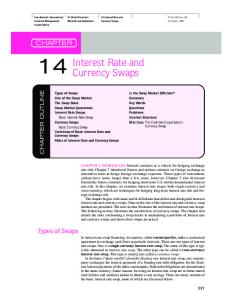
Netting A netting agreement between two parties is a part of the ISDA Master Agreement3 , which is an established framework for governing OTC transactions between counterparties. Netting, or more specific closeout netting, is a key way of mitigating counterparty credit risk and is simply an o↵setting of positive and negative cash flows. In the case where no netting agreement is in place, the potential loss of the surviving party will be the sum of counterparty exposure towards the defaulting counterparty. This sum will be posted as a claim in the bankruptcy process alongside the claims from other creditors, and will be recovered depending on the value of the remaining assets of the defaulting party. The surviving party would further have to fulfill all its financial obligations towards the defaulting party, and is una↵ected by the default of the counterparty. However, when there is a netting agreement in place, positive and negative cash flows towards the given counterparty will o↵set each other, causing the two payments to be reduced into one net payment. In the event of default, netting is beneficial for the surviving party as it potentially lets them retrieve (parts of) their outstanding value of the assets. If the net payment is negative for the counterparty, the event of default will not cause the surviving party any additional losses.

T

No netting Positive cash flows Negative cash flows

+50 +110 +60 +70 +110 +70 +50 -70

-90

-70

With netting Cash flow

+50 +40 +60 -20 +110

0

+50

Figure 2.1: Netting concept Collateral Furthermore the ISDA Master Agreement might be supported by a Credit Support Annex (CSA). This is related to posting of collateral (margining) and/or an independent amount. The former is most used, but they are both further ways of reducing counterparty credit risk. The CSA can for instance say that collateral have to be posted once the entire portfolio exposure with a given counterparty reaches a pre-determined threshold. If this threshold is set to zero, collateral has to be posted by the counterparty as soon as the exposure turns positive. If an independent amount is posted, the exposure will be limited 3

The ISDA Master Agreement is published by the International Swaps and Derivatives Association and outlines the terms applied to a derivatives transaction between two parties.

2.4. CREDIT VALUE ADJUSTMENT (CVA)

12

to the level above this amount. The CSA will further normally include aspects related to the timing and frequency of collateral postings, as well as what kind of collateral is to be posted. Preferred collateral is typically cash or liquid securities such as government bonds. Any exposure below the threshold specified in the CSA is not collateralized and is thus at risk in the case of counterparty default. Exposure above is collateralized and does therefore not face the same risk. In the event of default the surviving party will claim the collateral posted, and if this is enough to cover the entire positive exposure after netting, the net loss is zero. Additionally, there might be a time-lag between the last collateral posting and the time of default. During this time increment, the value of the portfolio might change. This is called gap risk. If the market moves a lot between the last collateral posting and default of the counterpart, this could lead to a substantial loss. With the introduction of collateral, independent amount and threshold in place, we can expand definition 2.1 to also include these mitigation tools Definition 2.2: Counterparty Exposure (Ex) In the case of collateral postings over the threshold H, we can define Ex(t) as Ex(t) = max (min (H, V (t)) , 0) When the contract includes a threshold H and independent amount IA in addition to the collateral posted above the threshold H, the exposure is Ex(t) = max (V (t)

2.4

IA, 0)

Credit Value Adjustment (CVA)

A basic and traditional way of handling counterparty credit risk is the use of credit limits, and making sure that the PFE of a given counterparty is not exceeding the set limit. The choice of the credit limit may vary according to the counterparty in question and risk preference, and it might also be time-dependent. The idea is that trades that will make the PFE breach the credit limit will typically not be accepted. However, using credit limits as a deciding measure whether the risk towards a counterparty is too high or not, is a rather static form of counterparty risk management. It does not incorporate any dynamical decision-making related to the probability and correlation of counterparty default, recovery rate or likelihood of credit downgrade. As these factors are likely to influence the determination of the credit limit in one way or another, a more general and dynamic approach for appraising the price of counterparty risk is likely to yield a better way of handling CCR. The solution to these issues is the credit value adjustment. CVA is the measure of including the monetary value of CCR when pricing contracts. For the contract value to reflect

2.4. CREDIT VALUE ADJUSTMENT (CVA)

13

its true value, it must include the probability and following consequences of the counterparty defaulting. This adjustment of the risk-free contract value is the CVA. Since the CVA is the di↵erence between the risk-free and risky value of a contract, it can intuitively be thought of as the market price of counterparty credit risk. CVA = Risk-free value - Risky value CVA moves beyond the binary world of credit limits, where the decision to accept a trade is determined according to whether the credit limit for the given counterparty is breached or not. By actually pricing in the risk and consequences of default via the CVA, the decision whether to include the trade or not is determined whether the profit of the trade covers the additional CVA from the trade. In practice, many adjustments can be made to the risk-free value of a contract in addition to CVA. Examples are debit (DVA), funding (FVA), liquidity (LVA) and margin (MVA) value adjustments. These are all abbreviated by the term xVA. We will however limit our focus to the credit value adjustment in this thesis. We will further assume that the party we are considering (typically a bank) is default-free. This means that we are considering unilateral CVA. The alternative approach is bilateral CVA where the party itself has a non-zero default probability. A further discussion of this is provided by Gregory [34]. CVA Formulation Unilateral CVA is the risk-neutral expectation of the discounted loss incurred if the counterparty defaults at some future time between today and a time horizon T . Definition 2.3: Credit Value Adjustment CV A(t = 0) = CV A(0) = (1

R)N (0)

Z

T 0

ENt



V + (t) ✏ = t dP D(0, t) N (t)

Here R is the recovery rate, given as the percentage of the outstanding value with the counterparty that is expected to be recovered in the case of the counterparty defaulting. (1-R) is consequently the loss given default, the amount assumed to be lost in the default event. Furthermore, ENt [. . . |✏ = t] is the time-t expectation conditional on default time ✏ = t under the probability measure N corresponding to the numeraire N (t). The CVA is independent of the probability measure N as it is a price adjustment. V + (t) is the counterparty exposure as defined in 2.1 and P D(s, t) denotes the probability of counterparty default between two times s and t. As we will see in section 6.1 this can be found by using market quoted credit spreads. If we further assume that there is independence between the exposure towards a counterparty and the credit quality of the counterparty (no wrong-way risk, see below), the expression above simplifies. In the expectation we do no longer need to condition on default time, thus the Z T  + V (t) CV A(0) = (1 R)N (0) ENt dP D(0, t) (2.2) N (t) 0

2.4. CREDIT VALUE ADJUSTMENT (CVA)

14

The standard discretization of (2.2) given in Gregory [34] is stated below. CV A(0) ⇡ (1

R)

m X

DF (ti ) EE (ti ) PD (ti

1 , ti )

(2.3)

i=1

in which DF is the relevant discount factor used to discount the future cash flows. CVA as an Option Given the definitions above, we return to our statement in the introduction claiming that the CVA can in fact be regarded as an option itself with the portfolio of trades as the underlying. The reason is simply that in case of counterpary default, the financial consequences (i.e. the option payo↵) will depend on the portfolio value to the surviving party. If this value is positive, the surviving party will only recover a fraction R of the outstanding value. If the value is negative however, they must fulfill all their monetary obligations to the defaulting party. It is precisely this asymmetry that gives rise to CVA and pricing it as an option. The option is American since default can happen at any time, and of the same reason the maturity of this option will be unknown. Looking at CVA this way, it is clear that it must also be priced the way one would price a ”normal” derivative contract. Wrong Way Risk (WWR) An important assumption we make in this thesis is that the counterparty�s probability of default is independent from the level of the exposure towards the counterparty. The situation where there is a positive correlation between the two, i.e. the probability of default increase when the exposure increase and vice versa, is called wrong-way risk (WWR). The opposite case where probability of default is low when exposure is high (and vice versa) is called right-way risk (RWR). Various attempts have been made to correct quantify and incorporate WWR in CVA calculations, including the works of Hull and White [40], B¨ocker and Brunnbauer [21] and Rosen and Saunders [58]. However, there is still no standard approach that is widely accepted by the industry, and WWR will not be included in our CVA calculations.

Chapter 3 Introduction to Interest Rates and Derivatives This chapter is intended for readers without prior experience to interest rates and interest rate derivatives. We start with a section on interest rate and interest rate derivatives basics under the traditional singe yield-curve setup, before we introduce the post-crisis two-curve setup which we implement in our Cheyette model.

3.1

Interest Rate Basics

This section contains a basic introduction to discount factors, forward rates and xIBOR rates under a single-curve setup. We start by defining basic financial assets such as zero coupon bonds (ZCB) and show how they represent the building blocks of interest rate modelling.

3.1.1

No-Arbitrage Pricing and Numeraires

A complete presentation of the building blocks of the theory of arbitrage free pricing is not in the scope of this thesis. For a thorough discussion on self-financing portfolios, absence of arbitrage, probability measures and martingales we refer the reader to Bj¨ork [17] and Cont and Tankov [30] which also serves as our main sources for this part. We consider an asset which is driven by a price process ⌘(t). In the theory of no-arbitrage pricing the time-t value of this asset ⇧(t) = ⇧(t, T, ⌘(t)), can be obtained by the use of numeraires. Roughly speaking we say that a numeraire N (t) is a positively priced asset which denominate other assets and facilitate comparison of the relative value of di↵erent assets. The time-t value of the asset is given by an expectation under an equivalent martingale measure N conditional on the filtration Ft , or the information available at time t. Hence, we have that ⇧(t) is defined by the expression  N ⇧(T ) ⇧(t) = N (t)Et (3.1) N (T ) For example if the numeraire is selected to be the money market account B(t), the price of the contingent claim is given by

3.1. INTEREST RATE BASICS

16

⇧(t) =

B EQ t



B(t)

⇧(T ) B(T )

Here QB denotes the equivalent martingale measure such that

(3.2) ⇧(t) B(t)

is a martingale.

In many areas of pricing it is often assumed that the instantaneous rate or short-rate r(t), at which the risk-free money-market account accrues, is a constant or a deterministic function of time. In the standard Black and Scholes option pricing formula one assumes that the short-rate is constant, as the main driver of the option price will be the movements of the underlying. However, in the context of pricing products where the main variability stems from the movements of interest rates, the probabilistic nature of the interest rates themselves is what matters the most. It is therefore necessary to consider a stochastic setup for the evolution of r(t). Definition 3.1: Money Market Account The stochastic money market account B(t) at time t is given by ⇣Z t ⌘ B(t) = exp r(s)ds

(3.3)

0

Let P (t, T ) denote the price at time t of a risk free contract which pays its face value of 1 at maturity at T , such that P (T, T ) = 1 with certainty. The contract, also known as a zero coupon bond, does not involve any periodic coupon payments. Thus, the arbitrage-free price of this contract is only the time-t expectation of the stochastic discount factor.   ⇣ Z T ⌘ B(t) QB QB P (t, T ) = Et = Et exp r(s)ds (3.4) B(T ) t

Furthermore, as we assume that the contract is risk-free (no default) the price of a ZCB can be viewed as a measure of the value of a future unit payment. ZCBs can therefore be scaled to fit the value of any future cash flow and the price P (t, T ) is therefore often referred to as a discount factor between a given time t and future time T . If we assume that the price process ⌘(t) is independent of the short-rate r(t), which is often assumed for equity prices, we see that equation (3.2) is just  ✓ Z T ◆ ⇤ B⇥ QB ⇧(t) = Et exp r(s)ds ⇧(T ) = P (t, T )EQ ⇧(T )|F (3.5) t t t

However, when dealing with interest rate derivatives we cannot assume independence and we can therefore not separate the expectation1 . Thus, in the case of a interest rate dependent derivative the expression (3.6) becomes difficult to evaluate as it involves two terms that both depend on the value of the underlying price process. This can be solved through what is known as the change of numeraire technique. We are allowed to change the numeraire N (t) ! N 0 (t), but this also involves a change of probability measure. The Girsanov theorem [32] implies that there exists a martingale measure N0 such that 1

If two stochastic variables X and Y are independent. The expectation E[XY ] is given by E[X]E[Y ].

3.1. INTEREST RATE BASICS

⇧(t) = N

17

0

0 (t)ENt



⇧(T ) N 0 (T )

(3.6)

Where N0 is the probability measure making N⇧(t) 0 (t) a martingale. Using the bond price P (t, T ) as our numeraire corresponds to the T -forward measure QT . Since P(T,T) = 1, we have that  ⇧(T ) QT ⇧(t) = P (t, T )Et (3.7) P (T, T )

The Girsanov theorem states that changing measure involves a drift adjustment of the stochastic process driving P (t, T ). We will later elaborate on how the drift adjustment is actually done.

3.1.2

Zero Coupon Term Structure

With the time-0 forward bond price denoted P0 (T1 , T2 ), with the special case of Pt (t, T ) = P (t, T ), we can through a simple no-arbitrage argument show that P (0, T ) = P (0, t)P0 (T1 , T2 ) ) P0 (T1 , T2 ) =

P (0, T ) P (0, t)

(3.8)

Thus, given that we can observe the market price of P (0, t) for di↵erent times t, we can easily calculate the forward price P0 (T1 , T2 ). Another interesting quantity is the continuously-compounded spot interest rate R(t, T ) which is the constant rate at which an investment of P (t, T ) at time t accrues continuously to pay a unit amount at maturity T . P (t, T ) = exp( R(t, T )(T

t)) ) R(t, T ) =

ln P (t, T ) T t

(3.9)

Knowing the current market price of P (0, T ) for di↵erent maturities T the mapping of ZCB to the corresponding interest rates T ! R(t, T ), is known as a the zero-coupon curve or a zero coupon term structure.

3.1.3

Forward Rates

Roughly speaking we can say that a forward rate reflects the price of a loan between two future dates. Forward rates are interest rates that can be locked in today for a certain future time period. Forward rates are characterized by three di↵erent points in time; the current time t at which the forward rate is considered, its expiry T1 and maturity T2 for which t  T1  T2 . The simply compounded forward rate is given by the relation ✓ ◆ 1 P (t, T1 ) F (t; T1 , T2 ) = 1 (3.10) (T2 T1 ) P (t, T2 ) By letting T2 ! T1 we obtain the instantaneous forward rate at time t for the maturity T1 as f (t, T1 ) =

@ ln (P (t, T1 )) @T1

(3.11)

3.1. INTEREST RATE BASICS

18

Instantaneous forward rates are fundamental quantities in interest rate modelling. Later we will see that one of the most flexible frameworks for interest rate modelling rely on the modelling of instantaneous forward rates. By reintegrating we see that we alternatively can express the ZCB prices as a functional of the instantaneous forward rate. Z T1 P (t, T1 ) = exp f (t, u) du (3.12) t

The information embedded in forward rates is exactly the same as in the prices of ZCB, as knowledge of ZCB prices implies what the forward rates are and vice versa. The instantaneous short rate at time t is also related to the instantaneous forward rate through r(t) = f (t, t)

3.1.4

(3.13)

xIBOR Rates and Day-count Conventions

The xIBOR rate is an official benchmark rate which is a reference for the average rate banks o↵er to lend unsecured funds to other banks. xIBOR is an abbreviation for the x Interbank O↵ered Rate, where the x usually refers to the first letter of the capital of the country or just just the first letter of the country in which the entity that fixes the rate resides. Examples are LIBOR, EURIBOR and NIBOR which are fixed by the British Bankes Association, The European Central Bank and the Oslo Bors Stock Exchange, respectively. Most interest rate derivatives are written on these official floating interest rates with varying maturity, e.g. EURIBOR3M is fixed for every third month. The maturity or tenor of these benchmark rates can range from a single day up to 12 months. EURIBOR rates are simply-compounded rates, typically linked to ZCB prices through a given day-count convention. For practitioners it is important to note that day-count conventions and market practice can vary between countries and contracts. As a complete description of di↵erent day-count conventions is not in the scope of this thesis, we will limit ourselves by just describing our chosen day-count fraction2 for this thesis, which is the 30e/360 convention. In this convention, also called the Eurobond basis, a year is assumed to be 360 days long, and a month is always assumed to have 30 days. If either the first or second date falls on the 31st , it is changed to 30. The EURIBOR rate can be defined as either a spot or a forward interest rate. The simply compounded spot EURIBOR rate at time t is defined as L (t, T ) =

1 P (t, T ) ⌧ (t, T )P (t, T )

for 0  t  T

(3.14)

Here ⌧ (t, T ) is the year-fraction between time t and time T in the day-count convention used. Whereas the the simply compounded forward EURIBOR rate is defined by ✓ ◆ 1 P (t, T1 ) F (t; T1 , T2 ) = 1 for 0  t  T1  T2 (3.15) ⌧ (T1 , T2 ) P (t, T2 ) 2

A brief discussion of di↵erent day-count conventions is given by Brigo and Mercurio [23]

3.2. INTEREST RATE DERIVATIVES

3.2

19

Interest Rate Derivatives

In the following we will give a brief description of the dynamics and cash flows related to fixed and floating rate bonds, interest rate swaps, interest rate caps and swaptions. The main source of this section is Brigo and Mercurio [23].

3.2.1

Fixed Rate Bond

A fixed rate bond is an instrument which at each time Ti pays a coupon given by a fixed rate ⇡ of a notional amount A, and at maturity Tm = T¯ also pays the notional itself. We denote ⌧i = Ti Ti 1 and obtain the payments ( ⌧i A⇡ i 2 1, 2, . . . , m 1 Z f ixed (Ti ) = ⌧m A⇡ + A i = m Thus the time t  T¯ value of the fixed rate bond is given by the following expectation under the T¯-forward measure. V

f ixed

¯

T (t) = P (t, T¯)EQ t

X m i=1

3.2.2

Z f ixed (Ti ) P (Ti , T¯)

Floating Rate Bond

A floating rate bond di↵ers from the fixed rate bond in that the coupon payments are determined by a floating rate, for instance the EURIBOR rate L(Ti 1 , Ti ) instead of a fixed rate ⇡. ( A⌧i L(Ti 1 , Ti ) i 2 1, 2, . . . , m 1 Vif loating (Ti ) = A⌧m L(Tm 1 , Tm ) + A i = m Similarly to above, we can derive the time t value of these payments. V

f loating

¯

T (t) = P (t, T¯)EQ t

X m i=1

3.2.3

Z f loating (Ti ) P (Ti , T¯)

Plain Vanilla Interest Rate Swap (IRS)

A plain vanilla interest rate swap is an agreement where two parties agree to exchange a fixed flow (fixed leg) of interest payments against a floating flow (floating leg) of interest payments. The payments exchanged are interest on a notional amount A. When both legs are in the same currency, the notional is itself usually not exchanged, only the accrued interest. The payments are exchanged on predetermined dates in a predetermined time period, specified in the IRS contract. The party paying the fixed leg is said to have entered a payer swap while the party paying the floating leg and receiving the fixed leg have entered a receiver swap. In a swap agreement, the floating leg is typically linked to some benchmark rate, like LIBOR or EURIBOR. In addition there might be a spread on top, such that the floating

3.2. INTEREST RATE DERIVATIVES

20

leg could be quoted in the format of LIBOR + 50 basis points. The floating rate is set at some time (the reset date) before the actual payments are exchanged (settlement date). At every reset date throughout the life of the swap, a new floating rate becomes e↵ective. The value of the floating rate at the reset date then determines the size of the floating leg for the following accrual period. To find the value of the receiver and payer swap payments, as well as the par swap rate S, we replicate the position by noting that the cash flows can be replicated by the use of fixed and floating rate bonds respectively. We first look at the payer swap, where the holder of the contract pays the fixed rate ⇡ and receives the floating rate. This position is equivalent to paying a fixed rate bond and receiving a floating rate bond. Assuming that the floating-leg rate reset at dates T↵ , T↵+1 , . . . , T 1 and the float payments are made at T↵+1 , T↵+2 , . . . , T the value of a payer swap is given by V payer (t) = P (t, T↵ )A

P (t, T )A

X

⇡P (t, Ti )A⌧i

(3.16)

i=↵+1

where ⌧ is the year fraction according to the relevant day-count convention. The value of the receiver swap is derived in a similar way, only now the position is equal to paying a floating rate bond and receiving the fixed bond V receiver (t) = P (t, T )A

P (t, T↵ )A +

m X

⇡P (t, Ti )A⌧i

(3.17)

i=↵+1

Knowing the expression of both the fixed and floating leg of the swap, we can find the par swap rate S making the value of the fixed and floating payments equal such that the swap value zero. S(t, T0 , TM ) =

P (t, T↵ ) P (t, T ) P P (t, Ti )⌧i

(3.18)

i=↵+1

3.2.4

Interest Rate Cap/Floor

An interest rate caplet/floorlet is a derivative in which the payo↵ is specified by a benchmark rate and a strike K. The payo↵ equals the di↵erence between the strike and the level of the benchmark if positive, and zero otherwise. The payo↵ is in other words equivalent to a European call/put option on the benchmark rate, i.e. XTCaplet = max (L(Ti , Ti 1 ) i

K, 0) A⌧i

(3.19)

XTFiloorlet = min (L(Ti , Ti 1 )

K, 0) A⌧i

(3.20)

where A is the notional amount and ⌧i = Ti Ti 1 . Moreover, an interest rate cap/floor is a stream of interest rate caplets/floorlets. Caps are frequently used by borrowers to hedge the risk of increasing interest rates. If rates increase above K, the received payo↵ from the contract will compensate for the increased interest the buyer/borrower has to pay. It thus places a roof for the floating interest payment.

3.3. TWO-CURVE SETUP

3.2.5

21

Capped Swap

An interest rate swap is combined with an interest rate cap is known as a capped swap. The representation of a capped swap is similar to the plain vanilla swap, but the floating leg is capped to a certain predetermined level(s), such that the capped leg payments are given by Vicapped (Ti ) = max (L(Ti , Ti 1 ), K(Ti )) A⌧i One will often adjust the fixed rate of the capped swap to include the premium such that the swap is traded at-the-money. The value of the capped swap can be found a replicating portfolio consisting of a long position in a corresponding vanilla swap and short position in an interest rate cap.

3.2.6

Swaption

In a plain vanilla swaption, the holder has the right to enter a swap contract with predetermined specifications at the swaption maturity. The entered swap can be either a payer swap or a receiver swap, and the corresponding option is thus either a payer swaption or a receiver swaption. As the equivalent call option, the swaption can be of the European, Bermudan or American type. In the European case, the holder of the payer swaption will exercise the swaption at maturity if the value of the underlying swap is positive. We will elaborate more on the swaption payo↵ definition and swaption valuation in section 5.5 regarding verification of our stochastic interest rate model.

3.3

Two-Curve Setup

In the pre-2008 financial environment, one would say that the probability of a EURIBORrated bank to lose its rating was practically equal to zero. This would implicate that the yield of a 12-month bond would be the same as entering a 6-month contract and subsequently another 6-month, e↵ectively P (0, 12M ) = P (0, 6M )P (6M, 12M ), in line with the no-arbritrage argument we saw in equation (3.8). The post-crisis market assess this di↵erently, as discussed in Bianchetti [15] and Mercurio [52]. As a EURIBOR-rated bank may very well lose its rating after 6 months, the 12-month contract is traded at a higher yield than a contract entering the 6-month spot rate and the 6-month-to-6-month forward rate (the forward contract ensures the EURIBOR rate). Consequently, there is in a simulation based setup a need for separate curves for risk-free discounting and EURIBOR fixings, as opposed to the traditional single-curve setup. A common practice in the euro interest rate derivatives market today is to utilize two separate yield curves; one derived from overnight index swap (OIS) quotes used for discounting, and one derived from the euro-swap quotes for EURIBOR fixings.

3.3.1

Overnight Index Swap (OIS)

An overnight index swap (OIS) is an interest rate swap where the floating leg is tied to some overnight rate index. An example of such an index rate is the Federal Funds Rate, which is the rate for overnight unsecured lending between banks in US dollars and serves as an important benchmark rate. According to Hull and White [41] the OIS rate currently

3.3. TWO-CURVE SETUP

22

serves as the best proxy for the risk-free rate when valuing derivatives, rather than the LIBOR rate which has been market standard prior to the financial crisis of 2007-08. The rates derived from the OIS curve can therefore be used to compute risk free discount factors.

3.3.2

Building an EURIBOR Bond Curve

The EURIBOR swap rate in the two-curve setup at time t can be expressed as S(t, T0 , Tm ) =

P V f loat (t) BpV f ixed (t)

(3.21)

in which T0 and Tm are the start time and the maturity of the swap contract, respectively. P V f loat (t) is the present value at time t of the floating leg, and BpV f ixed (t) is the basis point value of the fixed leg at the same time. In this setting we define PV

f loat

(t) =

m X1

⌧if loat FEur (t, Ti , Ti+1 )POIS (t, Ti+1 )

i=0 m X1

BpV f ixed (t) =

(3.22) ⌧if ixed POIS (t, Ti+1 )

i=0

⌧if loat

f loat Ti+1

Tif loat

f ixed where = and ⌧if ixed = Ti+1 Tif ixed . POIS (t, Ti ) is taken to be the appropriate discount factor at time t for the maturity Ti , and is computed based on OIS quotes. Since the initial discount factor curve, POIS (0, Ti ) used in this thesis were provided by Danske Bank, we will not go further into detail on how to extract the OIS discount factors from the OIS quotes. FEur (t, Ti , Ti+1 ) denotes the arbitrage-free EURIBOR forward rates at time t, hence the variable that gives the payo↵ L(Ti ,Ti+1 ) ⌧Fi (t,Ti ,Ti+1 ) zero market value.

Furthermore, when we have a set of euro swap quotes and a set of risk-neutral discount factors, we can compute FEur (t, Ti , Ti+1 ). Having computed the forward rates, we can obtain the appropriate EURIBOR bond prices derived from the forwards by the following relation FEur (t, Ti , Ti+1 ) =

PEur (t, Ti ) PEur (t, Ti+1 ) ⌧i PEur (t, Ti+1 )

(3.23)

in which PEur (t, T ) is taken to be the bond price based on the EURIBOR spot rate with the given maturity. We can then solve for PEur (t, Ti+1 ) to get PEur (t, Ti+1 ) =

PEur (t, Ti ) 1 + ⌧i FEur (t, Ti , Ti+1 )

(3.24)

which can solved iteratively as we know that P (t, t) = 1 and that initially the forward rate is equal to the spot EURIBOR rate, i.e. FEur (t, t, T1 ) = LEur (t, T1 ).

Chapter 4 Interest Rate Models In general terms, an interest rate model can be said to be a probabilistic description of future evolution of interest rates, characterizing the uncertainty of future interest rates based on information available today. As most financial instruments have interest rate sensitive cash flows, the valuation of these derivatives will involve application of interest rate models. The selection and calibration of interest rate models, as well as the use of these models, are therefore important aspects for any trader, investor or portfolio manager in fixed-income markets. In the literature as well as in the practitioners world, there is a large variety of models available, each with their advantages and disadvantages. A tremendous amount of research has been done within the field of interest rate modelling and the literature contains a large set of di↵erent models. Trying to summarize this would be an immense task, but we will in the following give a brief review of the main lines. This review is mainly inspired by the presentation of interest rate models by Brigo and Mercurio [23]. Furthermore, the field of applications is broad. There is however no general agreement regarding which approach that yields the best results in any given market situation and for all applications. Nevertheless there exists a few common requirements which should be met for a practitioner to be able to rely on a given model. A discussion of these requirements, as well as a justification of our choice of the Cheyette model for this thesis is provided in section 4.4. Classification of Models Various attempts to model the evolution of interest rates can in general be classified into three di↵erent approaches; endogenous and exogenous short-rate models, models within the HJM-framework1 and market models. In particular we will focus on a separable HJM formulation presented in the pioneering work by Cheyette [28], Ritchken and Sankarasubrahmanyam [56], Babbs [13] and Jamshidian [42] known as Cheyette models. 1

Although virtually any exogenous interest rate model can be derived within the HJM-framework, we have decided to keep this classification of models due to clarity of presentation and their chronological appearance in the literature.

4.1. ENDOGENOUS AND EXOGENOUS SHORT-RATE MODELS

4.1

24

Endogenous and Exogenous Short-Rate Models

The earliest models for evolution of interest rates are the so called short-rate models. They all have in common that they model the dynamics of the instantaneous spot rate process of r(t) as defined in section 3.1. Modelling this spot rate, which is a non-observable variable, is very convenient as fundamental quantities such as rates and bonds are through no-arbitrage assumptions defined as expectations of functions depending on r(t). Defining the dynamics of r(t) and its distributional properties will characterize the entire zerocoupon curve through equation (3.4) and thus also any rate. In addition, short-rate models inhabit Markov properties. This is a desired property as it reduces the valuation problem for many instruments to solving a partial di↵erential equation (PDE) for which there exists analytical and numerical solving techniques. The selection of the driving process for the spot rate give rise to di↵erent versions of short-rate models. As an example, it was suggested in the seminal work by Vasicek [59] that the dynamics of r(t) could be governed by a mean-reverting Ornstein–Uhlenbeck process. Under the risk-neutral measure the dynamics of the spot rate under the Vasicek model is written as dr (t) = k[✓

r (t)]dt + dW (t) ,

r(0) = r0

(4.1)

Where r(0), k, ✓ and are all positive constants. As the stochastic di↵erential equation (4.1) is linear and the short-rate is Gaussian, we can solve it explicitly and find an analytical expression for the ZCB-price P (t, T ; k, ✓, , r(t)) (see [23] for more on this). However, a considerable disadvantage of such models is their endogenous nature. If we have an initial zero-coupon bond curve available from the market P M rkt (0, T ), we ideally want our model to incorporate this curve. This e↵ectively results in an optimization problem, where we seek to find the value of the model parameters such that the di↵erence between the model and market data is minimized. However, one will have difficulties with reproducing a given term structure satisfyingly even though P M rkt (0, T ) is only observed for a finite number of maturities. The inability to successfully fit an initial yield curve makes these models less attractive, but in order to improve on this problem a basic strategy is to transform an endogenous model into an exogenous model. This is done by inclusion of a time-varying parameter, and was first proposed by Ho and Lee [37]. In the case of the Vasicek model this can be done in the following way dr (t) = k[✓

r (t)]dt + dW (t) ! dr (t) = k[ (t)

r (t)]dt + dW (t)

(4.2)

(t) is chosen based on the market curve P M rkt (0, T ) such that the model reproduces exactly the current term structure of rates. The SDE in (4.2) is in fact a formulation of the well known Hull-White extended Vasicek model [39] (usually shortened to the HullWhite model). Other models of this type is the Black-Derman-Toy (BDK) [20] and the Black-Karasinski (BK) [19] models. Furthermore there exists multi-factor extensions of many short-rate models in order to accommodate a better fit to market data. However, this comes at the cost of less mathematical tractability and can also result in reduced stability of calibrated parameters. A general discussion of extensions to multi-factor models is provided in section 4.4.2 below. Using short-rate models to describe the evolution of interest rates have many advantages in terms of the large availability of di↵erent dynamics of the short-rate, as well as the

4.2. THE HEATH-JARROW-MORTON FRAMEWORK

25

Markov properties. Furthermore, the short-rate models are tractable and fairly easy to understand and implement. However, when valuing assets requiring information of longer rates this will be difficult for generic short-rate models like the BDT or BK. As stated by Cheyette [29] these models do not posses the desirable property that the entire forward curve can be expressed through fairly simple analytical formulas. Thus, a clear understanding of the covariance structure of the di↵erent forwards rates is difficult to achieve. This means that when valuing the individual contracts in a portfolio of interest rate derivatives, whose values depend on various forward rates, one cannot expect to use the same interest rate model in each valuation. It is however possible to show that the only exogenous short-rate models where one can obtain the entire forward curve analytically belongs to a class that includes models with the following short-rate volatility [44] (r, t) =

p a(t)r(t) + b(t)

where a(t) and b(t) are two deterministic, time-dependent functions. The Hull-White model [39] is special case of models in this class.

4.2

The Heath-Jarrow-Morton Framework

Another approach to modelling the evolution of interest rates is to define the dynamics of the entire yield curve. This is a significant advantage compared to just modelling the short-rate. In contrast to the short-rate models, models belonging to the framework put forth by the authors Heath, Jarrow and Morton (HJM) [36] are based on modelling the dynamics of the instantaneous forward rate rather than the short-rate and are sometimes referred to as whole-yield models. We emphasize that HJM should be thought of as a framework for interest rate models, rather than a specific model itself. Under the HJM-framework, the instantaneous forward rate is assumed to evolve according to the following di↵usion process df (t, T ) = ↵ (t, T ) dt + (t, T )> dW (t)

(4.3)

f (0, T ) = f M rkt (0, T )

W (t) = (W1 (t), . . . , WM (t)) is here a vector of Brownian motions of size M , where M is the number of stochastic factors included. The di↵usion coefficient (t, T ) = ( 1 (t, T ), . . . , M (t, T )) is an M-dimensional vector consisting of adapted processes. f M rkt is the market yield curve observed at t = 0. We will see next that the adapted process ↵(t, T ) is determined through the specification of the di↵usion coefficient (t, T ), as the dynamics described in (4.3) are not necessarily arbitrage-free. In order for a equivalent martingale measure to exist, certain restrictions apply to the forward rate drift ↵(t, T ). The relationship between the drift ↵(t, T ) and the volatility (t, T ) is in fact the central insight of the HJM-models. Specifically, under the risk-neutral measure, the drift must have the following structure ↵(t, T ) = (t, T )

Z

T

(t, s)ds = t

M X k=1

k (t, T )

Z

T k (t, s)ds t

(4.4)

4.3. MARKET MODELS

26

This yields the following dynamics of the instantaneous forward rate f (t, T ) under this measure Z t Z T Z t f (t, T ) = f (0, T ) + (u, T ) (u, s)dsdu + (s, T )dW (s) = f (0, T ) +

0 M XZ t k=1

u

k (u, T )

0

Z

0

T

k (u, s)dsdu u

+

M Z X k=1

(4.5)

t

k (s, T )dWk (t) 0

This expression tells us that the forward rates dynamics are entirely specified by its volatility structure (t, T ). Thus, choosing a particular model from the HJM-framework reduces to the choice of volatility structure for the forward rate (in addition to the initial yield curve f (0, T )). This is in contrast to the short-rate models where one can choose both the drift and volatility structures freely. The ability to specify di↵erent volatility structures for di↵erent maturities is also a key source of popularity for the HJM-models. From (3.13) the short-rate r(t) in the HJM-framework is defined as Z t Z t Z t > r(t) = f (t, t) = f (0, t) + f (u, t) f (u, s)dsdu + f (u, t)dW (u) 0

u

(4.6)

0

It is worth noticing that this short-rate process is not a Markov process. This precludes using PDE’s to value interest rate derivatives under the HJM-framework, and one has instead to rely on time-consuming simulations where the entire history of the interest rate evolution has to be dragged along. Since each forward rate of fixed maturity evolves separately, this leads to a high-dimensional stochastic process of the underlying. However, we will later discuss specifications of the di↵usion coefficient (t, T ) such that the shortrate process in the HJM-framework indeed becomes a Markov process.

4.3

Market Models

The third class of interest rate models we will present is the so-called LIBOR market model framework. They are called market models because of their compatibility with popular, fundamental market-formulas for two of the most traded interest-rate derivatives, namely caps and swaptions. The log-normal forward-LIBOR model (LFM) prices caps with Black’s cap formula and the log normal forward-swap model (LSM) prices swaptions with Black’s swaption formula respectively [18]. Besides this desirable convenience, market models have gained popularity as working directly with quantities that are actually quoted in the market and appear in derivatives payo↵ descriptions are more intuitive and natural than dealing with the instantaneous short-rate or the forward rate. The LFM approach first described by Brace et al. [22], Jamshidian [43] and Miltersen et al. [53] suggests the direct modelling of a finite set of simply compounded forward LIBOR rates. Under a given probability measure the forward LIBOR rate is in the LFM modelled as a driftless Brownian motion, whereas in the LSM it is the forward swap rate that is modelled as a driftless Brownian motion. Thus, dealing with models of this type will involve familiar Gaussian calculus. We will refer the interested reader to Brigo and Mercurio [23] for a more detailed description of the model dynamics.

4.4. CHOOSING AN INTEREST RATE MODEL

27

However, the non-Markovian nature of these models represents some implementation issues. There exists satisfying Markovian approximations, but the usual way of dealing with this is some rather computationally intensive Monte-Carlo simulations, as was the case for (most) models under the HJM-framework. Using these approximations one will have to deal with the estimation of complicated conditional expectations. Additionally, the inconsistency between the LFM and the LSM model is another drawback with this framework. It can be shown that the modelling of forward LIBOR rates as lognormal does not comply with the forward swap rate being lognormal in the LFM model [23]. Empirical evidence suggests that the forwards swap rates are not far from being lognormal, but the problem remains of choosing either of the two models for the entire market.

4.4

Choosing an Interest Rate Model

Given the large variety in ways of modelling the term structure of interest rates, the choice of which model to employ is not trivial. As stated in the beginning of this chapter, there is no general consensus amongst practitioners nor academics on a unified approach suitable for all applications. As of today, the market models mentioned above might be closest to achieving such a position. Despite their recent popularity however, we saw above that they still exhibit drawbacks that prevent them from being the preferred model for all cases, such as their non-Markovian nature. Models with a various degree of complexity are still being used for various purposes, and although interest rate models tend to get more and more complex, simpler models are still used for certain applications. From a practitioners view in particular there are certain requirements that should be fulfilled for a given interest rate model to be preferred, as mentioned in the introduction of this chapter. There is a rich discussion about this in the literature, including the works of Rogers [57] and Cheyette [29]. First of all the model should be flexible enough to fit market quotes of fundamental assets when calibrating in various market states. A flexible model is also more likely to give a satisfying volatility smile fitting, which is a desired property for an interest rate model. The interest rate model must furthermore be simple enough to provide efficient valuation algorithms for relevant financial contracts so that prices can be computed within reasonable time. Interest rate modelling is often performed by simulating a large number of scenarios, and the time horizon can be long. An efficient implementation is therefore important in order to keep the computational time within an acceptable range. Moreover, by having analytical valuation expressions available, calibration of the model is easier which is a significant advantage. In addition the model should be well specified such that the required parameters and inputs can either be observed directly or at least estimated in a reasonable manner. Finally the term structure must be realistic in the way that it is able to generate a realistic evolution of the yield curve. Again, this is especially important for interest rate modelling as one is often encountering long time horizons, which in turns leads to a large set of outcomes for the future market states.

4.4.1

The Cheyette Model

Given our purpose of computing CVA calculations on a portfolio of interest rate derivatives, we will naturally seek an interest rate model that complies with the above-described

4.4. CHOOSING AN INTEREST RATE MODEL

28

requirements. A specific model that we find suitable is the Cheyette model [28]. The model has its origins from the HJM-framework discussed above, and is specified by restricting the volatility structure (t, T ) of the forward rates to be separable into time and maturity dependant functions2 . This allows for a desirable Markov representation of the yield curve dynamics, which we will be elaborated below. A key reason for choosing the Cheyette model is the mentioned possibility of specifying it as a Markov process. By imposing the separable condition on the volatility, the model is Markovian in a finite number of state variables, as opposed to what is the case if the volatility structure is arbitrary specified[14]. This yields extensive benefits when applying valuation methods such as Monte-Carlo methods and valuation via partial di↵erential equations. As we mentioned in the previous section, one has to carry the entire history of simulated state variables to obtain the yield curve at a current point when using MonteCarlo in a non-Markovian structure. This path dependency increases the computational complexity considerably, which is not desirable when performing CVA calculations. Although calibration is not in the main scope of this thesis, the quick and accurate calibration of the Cheyette model also make it a preferable choice for interest rate modelling [45]. The model yields satisfying results when calibrated to both swaptions and caps. An important reason for this efficient calibration is the availability of closed-form pricing of caps and swaptions given by the Cheyette model. Furthermore, Hoorens [38] shows how a displaced di↵usion stochastic volatility (DDSV) formulation of the Cheyette model can efficiently be calibrated to the swaption market. Calibration of the Cheyette model is also discussed in Beyna [14] who implements several minimization algorithms in order to develop his calibration method3 . Furthermore, the Cheyette model is also popular because of its ability to incorporate stochastic volatility in a satisfying way. By including stochastic volatility, the model is able to match the market observed volatility smiles to a greater extent. According to Jesper Andreasen [45] the often preferred SABR-model [35] for stochastic volatility is difficult to handle when applied to full yield curve models. Instead they use the approach outlined by Andreasen and Andersen [10] to include stochastic volatility in the Cheyette model. This yields good results in terms of fitting the model to observed prices for swaption and caps. Although the benefits of including stochastic volatility is not exploited and implemented in this thesis, the Cheyette model’s compatibility of doing so makes it an attractive model choice. Finally, the strength of the Cheytte model is confirmed by its endorsement from practitioners Jesper Andreasen [45] as well as Andersen and Piterbarg [7]. They state that this class of models is among the best models for its purpose in their opinion. This is due to their ease of calibration, flexibility of volatility smile specification and the possibility of efficient numerical implementation. 2

The same model specification was also proposed by Babbs [13], Ritchken and Sankarasubrahmanyam [56] and Jamshidian [42]. 3 Beyna uses a slightly di↵erent formulation of the Cheyette model than we implement by imposing a parametric restriction of the functional form of the volatility.

4.4. CHOOSING AN INTEREST RATE MODEL

4.4.2

29

Choosing Factors

An important aspect of choosing a term-structure model is the number of stochastic factors to incorporate. Choosing factors represents a trade-o↵ between model flexibility and computational efficiency. The simplest case with one factor o↵ers a very simple model with good tractability, but will only be able to produce yield curves with deterministic, time-dependent shapes. With only one stochastic factor driving the entire yield curve, the interest rate for all maturities will be perfectly correlated. This means in turn that a shock to the interest rate at a given time will be transmitted equally to all maturities, moving the entire curve in the given direction. The fact that one-factor models only allows for time-dependent parallel shifts of the yield curve will impose a significant limitation for valuation cases that are dependent on multiple rates on the curve. For some products however, the value only depends on one point on the curve and a one factor model can produce satisfying results4 . In most cases however, the chosen interest rate model should allow for a more realistic correlation structure between forward rates, and thus a multi-factor model is required. When discussing the shape of the yield curve, it is important to distinguish between deterministic contributions (from the time-dependent functions) and the stochastic contributions generated by the underlying factors. We can think of the stochastic factors in the model as interpolation points on the curve, which means that an increased number of factors will generate increased flexibility in the stochastically induced shape of the curve. In general, we can see that a two-factor model will be able to generate a stochastic shift in the slope of the curve, but not a stochastic concave or convex shape. This feature is however possible in a three-factor setup. By assuming a multi-factor term-structure model driving the movements of the various forward rates, Litterman and Scheinkman [49] performed a principal component analysis (PCA) on the US treasury yield curve and found three components that explained up to 97 % of all variance in the forward rates. These factors are connected to the level, slope and curvature of the curve, and later studies have further confirmed their findings [48]. However, all the mentioned studies came from periods when negative interest rates did not exist. This questions the relevance of the findings in the market conditions today, and motivates the need for an even more flexible setup. For instance, we can see that using a three-factor model would not be able to generate a curve like the OIS yield curve we experience today forward in time, which has a wave-like shape (see the curve for t = 0 in figure 4.1 below), unless the input curve inhabits the same kind of shape. A four-factor model, is however able to capture these kinds of shapes nicely, and is therefore the chosen number of factors in this thesis. In the following figures, we have plotted a set of Monte-Carlo based realizations forward in time of the yield curve for the four-factor Cheyette model and for the Hull-White model5 . Time to maturity has been chosen to lie between 1 month and 14 years, and the time points in question are the initial time up to five years with one year increments. We can see that the Hull-White yield curve dynamics are restricted to time-dependent parallel shifts, and the Cheyette model spans a larger space of possible market states than 4

According to Rebonato and Cooper [55] the only examples are caps and some cases of knock-outs. If choosing M = 1, the Cheyette formulation can be reduced to the Hull-White extended Vasicek model we saw in equation (4.2) in the previous section. 5

4.4. CHOOSING AN INTEREST RATE MODEL

30

the Hull-White. This underlines the benefits of a mulit-factor model. 0,012 t=0 t = 1Y t = 2Y t = 3Y t = 4Y t = 5Y

0,01

0,008

yield to Maturity

0,006

0,004

0,002

0

−0,002

−0,004

0

2

4

6 8 Time to Maturity

10

12

14

Figure 4.1: Realizations of the future yield curve generated by the Cheyette model

0,01 t=0 t = 1Y t = 2Y t = 3Y t = 4Y t = 5Y

0,005

yield to Maturity

0

−0,005

−0,01

−0,015

−0,02

0

2

4

6 8 Time to Maturity

10

12

14

Figure 4.2: Realizations of the future yield curve generated by the Hull-White model

Chapter 5 The Cheyette Model In this chapter we will present derivations of the Cheyette model which we have implemented. After revealing the Markov properties of the Cheytte model, we derive the original Cheyette model proposed by Cheyette [28]. The model utilize a separable volatility structure of the underlying dynamics to formulate a term-structure model in the HJMframework with the desired Markovian properties. Subsequently we extend the derivations to an alternative model specification put forth by Andersen and Piterbarg [7], namely the Quasi-Gaussian formulation, and finally we present our implemented model setup. Investigating Markov properties As we saw in section 4.2 the dynamics of the instantaneous forward rate under the riskneutral measure in the HJM-framework can be written as Z T > > df (t, T ) = f (t, T ) (5.1) f (t, u)dudt + f (t, T ) dW (t) t

and a short-rate on the form

r(t) = f (t, t) = f (0, t) +

Z

t f (u, t) 0

>

Z

t f (u, s)dsdu + u

Z

t f (u, t)dW (u)

(5.2)

0

We can see that the expression contains an infinite number of state variables and is not Markovian in general. For a Markov process we have P (X(s) 2 B|Ft ) = P (X(s) 2 B|X(t)) t  s

(5.3)

where B is the set of possible outcomes for X. Hence, the future value of X depends only on the value at time t, and not on the entire history Ft . We denote Z t > D(t) = f (u, t) dW (u) 0 (5.4) Z T > D(T ) = D(t) + f (u, T ) dW (u) t

Since an incremental shift in the variable t will a↵ect the whole path of the function f (u, t) and not only over the incremental time step, the expressions are non-Markovian, i.e.

5.1. ORIGINAL CHEYETTE FORMULATION

32

E(D(T )|D(t)) 6= E(D(T )|Ft )

(5.5)

Now, we choose a separable form of the volatility function f (t, T )

= g(t)h(T )

(5.6)

and the short-rate can be rewritten as Z t Z t ⇣Z t ⌘ > r(t) = f (0, t) + h(t) g(u) g(u) h(s)ds du + h(t) g(u)> dW (u) 0

u

(5.7)

0

D(T ) now only depends on D(t) and information arriving after t Z T Z T h(T ) > D(T ) = h(T ) g(u) dW (u) = D(t) + h(T ) g(u)> dW (u) h(t) 0 t

(5.8)

We can thereby see that with the given volatility specification, the dynamics in equation (5.1) inhabits Markov properties.

5.1

Original Cheyette Formulation

In this section we present the novel formulation of the Cheyette model presented by Cheyette [28] in order to obtain a starting point and motivation for the subsequent, implemented formulation.

5.1.1

Instantaneous forward rate dynamics

The instantaneous forward rate, f (t, T ), can be represented in the general M -factor HJMframework as df (t, T ) =

M X ⇥

k (t, T )

k=1

Z

T t

M X ⇤ (t, s)ds dt + k

k (t, T )dWk (t)

(5.9)

k=1

where W (t) denotes an M -dimensional Brownian motion under the risk-neutral measure. The model is entirely specified by the choice of volatility-structure { (t, T )}T t . The volatility-function takes the form of an M -dimensional vector 0 1 (t, T ) 1 C B .. (t, T ) = @ (5.10) A . M (t, T )

The volatility function of each factor is defined as k (t, T )

=

Nk (k) X ↵ (T ) i (k) i=1 ↵i (t)

(k) i ,

k = 1, . . . , M

(5.11)

where Nk denotes the number of volatility summands of factor k. With the given volatility structure, the forward rate can be formulated as

5.1. ORIGINAL CHEYETTE FORMULATION

f (t, T ) = f (0, T ) +

✓ (k) Nk M X X ↵j (T ) (k)

j=1

k=1

↵j (t)

(k) Xj (t)

+

33

Nk (k) X A (T )

(k)

Ai (t)

i

(k)

↵i (t)

i=1

(k) Vij (t)

◆

(5.12)

where the state variables are given as

(k) Xi (t)

=

Z

t

(k)

↵i (t)

(k) 0 ↵i (s)

(k) i (s)dWk (s)

+

Z

t

X Nk (k) i (s)

(k)

↵i (t)

(k) ↵i (s)

0

(k)

Aj (t)

j=1

(k)

Aj (s)

(k) ↵j (s)

(k) j (s)

ds

(5.13)

Furthermore, the deterministic time-functions are defined as (k) Vij

=

(k) Vji

(k)

Ai (t) =

Z

=

t 0

Z

t

(k)

(k)

↵i (t)↵j (t)

(k) (k) i (s) j (s)ds (k) (k) 0 ↵i (s)↵j (s)

(5.14)

(k)

↵i (s)ds

for k = 1, . . . , M and i, j = 1, . . . , Nk . The dynamics of the forward rate are in turn (k) determined by the state variables Xi (t), which are formulated as independent Markov processes by (k) dXi (t)

=

✓

(k) Xi (t)

t

i.e. we assume that

⇣

log

⇥

⇤ (k) ↵i (t)

⌘

+

(k) Vij (t)

j=1

hdWk , dWl i = 0,

5.1.2

Nk X

◆

dt +

(k) i (t)dWk (t)

(5.15)

k, l = 1, . . . , M

Volatility specification

In this section we examine the volatility specification of the originally formulated Cheyette model. As discussed in section 4.2, the dynamics of the instantaneous forward rate can be determined entirely by the volatility structure, given by equations (5.9) and (5.10). Beyna [14] proposes the following parametric form of the volatility structure i (t, T ) (i)

(i)

= P(i) m exp

i (T

t)

i = 1, . . . , M.

(5.16)

(i)

in which Pm = am tm + am 1 tm 1 + . . . + a0 . This volatility specification is consistent with the original Cheyette form where (1)

↵i (t) = exp(

(1)

t),

(1) i (t)

= P(i) m (t)

(5.17)

According to Beyna [14], one way to increase the accuracy of the model calibration would be to incorporate a constant term such that the volatility function will converge toward this value in the limit T ! 1. In particular, it is shown that the calibration to short

5.2. QUASI-GAUSSIAN CHEYETTE FORMULATION

34

maturities improve significantly with this approach. A multi-factor Cheyette model on this form gives a better fit to volatility skews and smile than for instance the Hull-White model, and will also in some cases provide analytical solutions to the SDE’s driving the processes. However, the model is restricted by the form of the volatility function, in addition to relying on the questionable assumption that the stochastic factors are independent, which ultimately reduces the flexibility of the model.

5.2

Quasi-Gaussian Cheyette formulation

Following Andersen and Piterbarg [7], we present an alternative formulation of the Cheyette model with no restriction of the functional form of the volatility, hereby denoted as the Quasi-Gaussian formulation. The extension comes at additional computational cost, as extra state variables are required to preserve the no-arbitrage condition of the model. The Quasi-Gaussian formulation combines the flexibility of volatility smile and skew specification with relative ease of calibration and efficient numerical implementation. In this setting volatility skew referes to market conditions where the implied volatility is either higher or lower for out-of-the-money options than in-the-money options. Consistent with the original Cheyette formulation, the Quasi-Gaussian is obtained by imposing a separability condition on the volatility structure of an HJM-model, although non-parametric. The section will start with a derivation of the one-factor model followed by a multi-factor extension.

5.2.1

One-factor Model

By choosing the following separable form of the volatility function, (t, !, T ) = g(t, !)h(T ), where g(t, !) is a one-dimensional stochastic process and h(T ) is a deterministic function, we can formulate the instantaneous forward rate by the following SDE ⇣Z > ⌘ > > df (t, T ) = h(T ) g(t, !) g(t, !) h(u)du dt + h(T )> g(t, !)> dW (t) (5.18) t

Now, we define the state variables x(t) and y(t) as dx(t) =

⇣ h0 (t) h(t)

⇣

⌘ x(t) + y(t) dt + h(t)g(t)dW (t),

dy(t) = [h(t)g(t)]2 + 2

0

⌘

h (t) y(t) dt, h(t)

x(0) = 0 (5.19)

y(0) = 0

Given the substitution of variables, x(t) and y(t), we can write the instantaneous forward rate as the solution to the SDE in (5.18) ! Z h(T ) y(t) T f (t, T ) = f (0, T ) + x(t) + h(s)ds (5.20) h(t) h(t) t Here, f (0, T ) = f mrkt (0, T ), hence taken to be the spot rate for various maturities. If we further introduce

5.2. QUASI-GAUSSIAN CHEYETTE FORMULATION

r (t, !)

=

r (t, x(t), y(t))

35

⌘ h(t)g(t, x(t), y(t)) (5.21)

h0 (t) h(t)

(t) ⌘ we get the following dynamics

dx(t) = y(t)

(t)x(t))dt +

r (t)dW (t)

(5.22) dy(t) =

r (t)

2

2(t)y(t) dt

y(t) is a locally deterministic, auxiliary variable upholding the no-arbitrage condition. By formulating the short-rate as r(t) = f (t, t), can see that x(t) perturbates the short-rate r(t) ⌘ f (t, t) = f (0, t) + x(t)

5.2.2

(5.23)

Multi-factor Cheyette model

Consider the instantaneous forward rate process df (t, T ) =

f (t, T, !)

>

hZ

T f (t, u, !)du t

i

dt + dW (t)

!

(5.24)

where f (t, T, !) is a d-dimensional stochastic process, and W (t) a d-dimensional Brownian motion under the risk-neutral measure. As for the one-factor case, we assume that f (t, T, !) is separable, so that we can rewrite it as f (t, T, !)

= g(t, !)h(T )

(5.25)

in which g(t, !) is a d ⇥ d stochastic matrix-valued process and h(t) is a d-dimensional deterministic vector-valued function of time. Now let 0 1 h1 (t) 0 ··· 0 B 0 h2 (t) · · · 0 C B C H(t) = diag(h(t)) = B .. (5.26) C .. . . @ . . . 0 A 0 0 0 hd (t) We further assume that hi (t) 6= 0, i = 1, . . . , d, which means that H(t) is invertible and we can define the diagonal matrix (t) by (t) =

dH(t) H(t) dt

1

(5.27)

Furthermore, we define G(t, T ) =

Z

T

H(u)H(t) 1 1du,

r (t, !)

= g(t, !)H(t)

t

where 1 = (1, 1, . . . , 1)> . Now, consider the processes x(t) and y(t) defined by

(5.28)

5.2. QUASI-GAUSSIAN CHEYETTE FORMULATION

x(t) = H(t)

y(t) = H(t)

Z

t

>

g(s, !) g(s, !) 0

⇣Z

t

Z

36

t

h(u)duds + H(t)w(t) s

(5.29) ⌘

g(s, !)> g(s, !)ds H(t)

0

where w(t) is a random d-dimensional vector satisfying dw(t) = g(t, !)> dW (t),

w(0) = 0

(5.30)

We can see that y(t) solves the system of ODE’s below dy(t) = H(t)g(t, !)> H(t) dt The state variables can thus be formulated as dx(t) = (y(t)1

(t))dt +

(t)y(t)

r (t)

>

y(t)(t)

dW (t),

(5.31)

x(0) = 0 (5.32)

dy(t) = ( r (t)

>

r (t)

y(t)

y(t)),

y(0) = 0

The instantaneous forward rate is thereby given by f (t, T, x(t), y(t)) = f (0, T ) + 1> H(T )H(t)

1

x(t) + y(t)G(t, T )

(5.33)

As in the one-factor case, f (0, T ) is taken to be the spot rate. The short rate is given as r(t) = f (t, t) = f (0, t) + 1> x(t)

(5.34)

Volatility specification In this section, we will present the general volatility structure in the Quasi-Gaussian formulation, with both a locally deterministic and a stochastic component. We start by defining a one-dimensional process z(t) by dz(t) = ✓(z0

z(t))dt + ⌘(t)dZ(t),

z(0) = z0 = 1;

(5.35)

with hdZ(t), dW (t)i = 0. We would like to specify a model with the following volatility specification > r (t, !) =

p z(t) x (t, x(t), y(t))>

(5.36)

in which x (t, x(t), y(t)) is a multi-dimensional local volatility function responsible for inducing the skews in volatility smiles for swaptions. It is, however, not obvious how to parametrize f (t, x, y) sensibly, as the volatility function is not only responsible for skews, but also for the general volatility structure of the model (including volatilities and correlations of all the rates). Defining d benchmark tenors 1 < . . . < d and subsequently the instantaneous forward rates fi (t) = f (t, t + i ), i = 1, . . . , d, a beneficial way to formulate the dynamics would be on an affine form in the forward rates

5.2. QUASI-GAUSSIAN CHEYETTE FORMULATION

37

⇣ ⌘ p dfi (t) = z(t) i (t) ↵i (t) + bi (t)fi (t) dUi + O(dt),

i = 1, . . . , d

(5.37)

where {Ui (t)}di=1 is a d-dimensional vector of Brownian motions with the correlation matrix X f (t) = { i,j (t)}, i (t) is a volatility calibration parameter, and ↵i (t) and bi (t) are parameters related to the volatility skews observed in the swaptions-markets. Now, let us define the following d ⇥ d process 0 1 h(t + 1 )> B C .. H f (t) = @ (5.38) A . > h(t + d ) f

and

f

(t, f (t)) by

(t, f (t)) = diag

⇣

1 (t)(↵1 (t)

+ b1 (t)f1 (t)), . . . ,

d (t)(↵d (t)

where f (t) = (f1 (t), . . . , fd (t))> . We further specify a structure of p > z(t) x (t, x(t), y(t))> r (t, !) = x (t, x(t), y(t))

>

= H(t)H f (t)

1 f

>

+ bd (t)fd (t)) r (t, !)

>

as

⌘

(5.39)

(5.40)

(t, f (t))Df (t)>

Df (t) is given by the Cholesky-decomposition of the matrix X f (t) = Df (t)> Df (t). X f (t) is taken to be the correlation matrix of the benchmark tenors, and the i (t)-parameters are specified for all benchmark tenors, which means that we can distribute volatilities out on factors. The bond reconstruction formula can in turn be written as

P (t, T, x(t), y(t)) =

⇣ P (0, T ) exp P (0, t)

G(t, T )> x(t)

⌘ 1 G(t, T )> y(t)G(t, T ) 2

(5.41)

Proof of bond reconstruction formula Defining M (t, T ) = H(T )H(t) 1 1, we can formulate the bond price as

P (t, T ) = exp = exp

⇣

Z

Z

T

f (t, u)du t

!

T

f (0, u)du t

⇣Z

⇣ P (0, T ) = exp G(t, T )> x(t) P (0, t)

T t

⌘

>

M (t, u) du x(t) Z T Z > M (t, u) y(t) t

u

Z

T

>

M (t, u) y(t) t

M (t, s)dsdu t

⌘

We identify that Z

T

>

M (t, u) y(t) t

Z

u

M (t, s)dsdu = t

Z

T t

@G(t, u) > y(t)G(t, u)du @u

Z

u

M (t, s)dsdu t

⌘

5.3. THE DISPLACED FOUR-FACTOR CHEYETTE MODEL

38

y(t) is symmetric, and matrix calculus shows that @ @G(t, u) > @G(t, u) > G(t, u) y(t)G(t, u) = y(t)G(t, u) + G(t, u)y(t) @x @u @u @G(t, u)> =2 y(t)G(t, u) @u Finally, we have that Z

T t

Z @G(t, u) > 1 T @ y(t)G(t, u) = G(t, u)> y(t)G(t, u) du @u 2 t @x 1 = G(t, T )> y(t)G(t, T ) 2

Calibration and Specification of Parameters The calibration of the model is linked to a set of swaption-quotes with various expiry and maturity. The i (t)’s are chosen so that the computed model volatility for the swaptioncontracts match with the implied volatility from Blacks formula quoted in the market. The maturities are chosen to coincide with the chosen benchmark rate tenors. The timeevolution of the i (t)’s are computed based on the di↵erent expiries of the swaptioncontracts, and each expiry constitutes a data point in time of the f (t)’s. We will not further go into detail of the calibration process, as calibration is not within the scope of this thesis. The remaining parameters are not computed from markets quotes, but simply given based on general assumptions of the market dynamics.

5.3

The Displaced Four-Factor Cheyette Model

The given formulation of the Cheyette model has utilized inspiration from the LIBOR Market Model. The LMM models each simply compounded forward rate simultaneously. The interpretation of the volatility is therefore intuitive, and is related to how much each factor in the model contributes to the forward rate’s volatility. One specific version of the multi-factor Quasi-Gaussian formulation is the four-factor case. Stochastic factors are chosen to span the term structure of interest rates, in which we have chosen the 6 months (6M), 2 years (2Y), 10 years (10Y) and 30 years (30Y) tenors.

5.3.1

Volatility structure

For the formulation stated above we end up with the following volatility structure 0

h1 ( Bh 1 ( B r (t) = @ h1 ( h1 (

1)

h2 ( 2 ) h2 ( 3 ) h2 ( 4 ) h2 (

1)

h3 ( 2 ) h3 ( 3 ) h3 ( 4 ) h3 (

1)

h4 ( 2 ) h4 ( 3 ) h4 ( 4 ) h4 (

1)

1

C A 3) 4) 2 )C

1

0

f 1 (t)

B 0 B @ 0 0

0 f 2 (t) 0 0

0 0 f 3 (t) 0

1 0 0 C C D> 0 A f 4 (t)

(5.42)

5.3. THE DISPLACED FOUR-FACTOR CHEYETTE MODEL

39

D is the Cholesky-decomposition of the correlation matrix X of the benchmark rates, and we choose hi (t) = exp( i t) to obtain the state variables on the familiar mean-reverting form, in which the 4 ⇥ 4 matrix (t) is given by 0 1 1 0 0 0 B 0 2 0 0 C C (t) =  = B (5.43) @ 0 0 3 0 A 0 0 0 4 The parameters in equation (5.39) are chosen to be bi (t) = b ↵i (t) = (1

(5.44)

b)f (0, t + i )

for i = 1, . . . , 4, where the constant b denotes the volatility skew parameter. In order to handle negative realizations of the instantaneous forward rate and keep the local volatility function positive, we incorporate a displacement parameter ⇣. The displaced, local volatility function is therefore stated as f

(t) =

p z(t)

f

(bf + (1

b)f0

⇣)

(5.45)

where f ⌘ f (t, ), f ⌘ f (t, t + ) and f0 ⌘ f (0, t + ). The variable z(t) is a onedimensional process governed by dz(t) = ✓(1

z(t))dt + ⌘(t)

p

z(t)dZ(t)

(5.46)

in which dZ(t) is a standard Wiener process, and the local volatility is thereby stochastic. This means that the volatility itself can experience shocks independent of shocks in the instantaneous forward rate, and e↵ectively yields flexibility in yet an additional stochastic dimension. However, we will proceed with ⌘(t) = 0, i.e. with a locally deterministic volatility structure. Recall the definition of G(t, T ) in equation (5.28), and the specification of the meanreversion parameters hi (t) = e

i t

i = 1, . . . , 4

(5.47)

G(t, T ) is therefore stated as a 4-dimensional vector on the form G(t, T ) =

5.3.2



1

e

1 (T t)

1

,

1

e

2 (T t)

2

,

1

e

3 (T t)

3

,

1

e

4 (T t)

4

>

(5.48)

Two-Curve Setup and Change of Measure

In the presentation of the four-factor Cheyette model above we have represented the dynamics of the model under the risk-neutral measure QB , with the money market account B(t) as our numeraire. Under this measure we model the OIS discount factors given by the bond reconstruction formula (5.41) as

5.3. THE DISPLACED FOUR-FACTOR CHEYETTE MODEL

POIS (t, T, x(t), y(t)) =

⇣ POIS (0, T ) exp POIS (0, t)

40

⌘ 1 G(t, T )> y(t)G(t, T ) (5.49) 2

G(t, T )> x(t)

in which POIS (0, t) and POIS (0, T ) denote the initial OIS discount factors for maturities t and T . Hence the initial OIS bond curve deduced from the OIS swap quotes, constitutes the input curve to the model. As we have a closed form expression for the POIS (t, T, x(t), y(t)) it would be convenient to use this as our appropriate discount factor, instead of having to evaluate the integral in (3.5). In the risk-neutral measure, the stochastic discount factor is given by ⇣ Z T ⌘ B(t) D(t, T ) = = exp r(s)ds (5.50) B(T ) t We can see, in particular that given (5.49)

POIS (t, T, x(t), y(t)) 6= exp

Z

⇣

T

r(s)ds t

⌘

(5.51)

Using POIS (t, T, x(t), y(t)) as the appropriate discount factor requires to change measure of the dynamics to the T -forward measure QT . This is done by utilizing the Radon-Nikodym [23] derivative given the filtration Ft , denoted as 0,T t

=

dQT dQ0

For this case, we get 0,T t

=

(5.52) Ft

B(0) B(t) P (0,T ) P (t,T )

(5.53)

in which its di↵erential in this case is given as d

0,T t

=

0,T t

r (t)G(t, T )dW

The solution of this SDE is taken to be ⇣ 1Z t t = exp r (s)G(s, T )ds 2 0 Identifying

r (t)G(t, T )

Z

0

(t)

t r (s)G(s, T )dW (s) 0

as the Girsanov kernel and defining dW T (t) := dW B (t) +

r (t)G(t, T )dt

(5.54) ⌘

(5.55)

(5.56)

we can see from Girsanov’s theorem, that W T (t) is a standard Brownian motion under QT . The drift corrected dynamics under the T -forward measure then becomes ⇣ ⌘ > d˜ x(t) = y(t)1 ˜ x(t) (t) (t)G(t, T ) dt + r (t)> dW T (t) (5.57) r r which result in the following expression for the OIS discount factors

5.3. THE DISPLACED FOUR-FACTOR CHEYETTE MODEL

⇣ POIS (0, T ) POIS (t, T, x˜(t), y(t)) = exp POIS (0, t)

41

⌘ 1 > G(t, T ) y(t)G(t, T ) (5.58) 2

>

G(t, T ) x˜(t)

It is important to notify that in the two-curve setup, the drift correction only applies to the OIS discount curve. When computing simulated EURIBOR bond prices, the state variables should therefore not be adjusted, as that would indicate that we are underestimating the drift of the actual payo↵s (since the rates are proportional to the state variables) from the derivative in question, which in turn gives a lower value than the true value of the derivative. The spread between the EURIBOR and OIS curves is assumed to be deterministic, and is computed based on the spot curves at time zero. Denoted on discount factor form, it is called basis, B(0, t), and can be computed by the following relation PEU R (0, t) = POIS (0, t)B(0, t)

(5.59)

where P (0, t) is the discount factor over the time frame [0, t] provided by the EURIBOR curve, and POIS (0, t) is the discount factor from the OIS curve. When computing the simulated EURIBOR bond price, PEU R (t, T ), we evaluate the bond reconstruction formula with the risk-neutral stochastic state variables with the appropriate scaling, i.e. ⇣ POIS (0, T )B(0, T ) PEU R (t, T, x(t), y(t)) = exp POIS (0, t)B(0, t)

>

G(t, T ) x(t)

⌘ 1 > G(t, T ) y(t)G(t, T ) 2 (5.60)

Numeraire Test Under the given probability measure, given the relation in (3.6), we should be able to reproduce the set of initial discount factors, POIS (0, Ti ) for all maturities Ti , by specifying a unit payment at Ti , which is discounted back to time zero using the appropriate numeraire, hence  1 N POIS (0, Ti ) = N (0)E0 N (Ti ) Using POIS (t, T¯, x˜(t), y(t)) as our numeraire N (t), we should be able to check if the numeraire have been constructed properly by using the fact that the ratio (5.61) should equate to one under the T¯-forward measure. Here T¯ is a horizon time chosen big enough to cover all cashflows relevant for the eventual pricing under consideration. POIS (0, Ti ) ⇤ =1 ¯⇥ N (0)ETt N (Ti ) 1

(5.61)

In the following plot, we can see the results from testing the accuracy of the discount factors under the two di↵erent measures described above. We have compared the results of using the simulated OIS bond prices directly as discount factors under the risk-neutral measure, with the drift adjusted OIS bond prices under the rward measure. Particularly, we can conclude that the bond price, POIS (t, T, x(t), y(t)), cannot be used as a discount

5.3. THE DISPLACED FOUR-FACTOR CHEYETTE MODEL

42

factor under the risk-neutral measure, as pointed out in equation (5.51). This would generate arbitrage opportunities relative to the initial discount factor over certain time periods, which is a violation with the no-arbitrage assumptions made in section 3.1.1. Furthermore, we see that the drift-adjusted OIS bond prices under the T -forward measure give substantially higher accuracy, although still with an observable error. This will be further discussed in section 5.5. 1.007 With drift correction Without drift correction

1.006 1.005 1.004 1.003 1.002 1.001 1 0.999 0

20

40

60 80 Months

100

120

Figure 5.1: Testing the simulated numeraire undter T¯-forward measure dynamics

5.3.3

Interpretation of the Stochastic Factors

In the four-factor case, the local volatility function related to each factor is given as f i (t)

=

p z(t)

f

(bfi + (1

b)f0i

⇣) i = 1, . . . , 4

The volatility structure of the stochastic factors is thereby dependent on the realizations of the benchmark rates. From the bond reconstruction formula in equation (5.41), we can see that the vector of weights, G(t, T )> , determines how much weight each stochastic factor constitutes in the bond price for a given (t, T ). Looking at the particular case of bond prices P (t, t + i ) for i = 1, . . . , 4, where G(t, t + i ) = G( i ), the dependency structure to the stochastic factors become quite apparent. For instance, when computing P (t, t + 2Y ), the weighting of x2Y (t) is higher than in the P (t, t + 6M ), which corresponds to the intuition behind the the factors. This relation is consistent throughout the tenors, as for instance the weighting of x30Y (t) is higher for P (t, t+30Y ) than for the P (t, t+10Y ) and P (t, t+2Y ) bonds. In terms of bond-price calculations, we can think of the stochastic factors as separate building blocks of the bond price. The magnitude of each factor-weight will therefore increase as the tenor increases. This is why x6M (t) has a higher weight (in absolute terms) in P (t, t + 30Y ) than P (t, t + 6M ).

5.4. PRESENTATION OF THE DATA

5.4

43

Presentation of the Data

In this section, we will present the input data used in the displaced four-factor Cheyette model, and discuss some practical issues regarding the implementation. The data was retrieved on March 31 2015, and provided by Nicki Rasmussen from the Counterparty Credit and Funding Risk desk at Danske Bank in Copenhagen.

5.4.1

Parameters

As briefly discussed in section 5.2.2, the -parameters are bootstrapped to a set of marketquoted swaption-premiums. By calibrating to the set of swaption-contracts ranging from one year to 20 years expiry and maturities consistent with the 6M, 2Y, 10Y and 30Y tenors, the time-evolution of i are given by i (t)

31.mar.16 31.mar.17 31.mar.18 31.mar.19 31.mar.20 31.mar.22 31.mar.25 31.mar.27 31.mar.30 31.mar.35

6M

2Y

10Y

30Y

0.277088665 0.432663473 0.478775455 0.526043695 0.569190886 0.423348024 0.61470724 0.419315568 0.36633221 0.538352429

0.375262617 0.370208663 0.387325279 0.351438297 0.302125887 0.330169421 0.317216441 0.344957612 0.157625833 0.19809944

0.419681129 0.443347904 0.398787776 0.368574909 0.382206147 0.348373918 0.383723704 0.486732797 0.317706939 0.404493446

0.593531387 0.478331979 0.419899231 0.286642116 0.230694637 0.143252904 0.06417227 0.441485524 0.05 0.05

Table 5.1: Calibrated (t) parameters

0.7 6M tenor 2Y tenor 10Y tenor 30Y tenor

0.6

0.5

λ(t)

0.4

0.3

0.2

0.1

0

0

2

4

6

8

10 t

12

14

16

18

20

Figure 5.2: Plotted -parameters for the 6M, 2Y, 10Y and 30Y tenors

5.4. PRESENTATION OF THE DATA

44

The remaining input parameters to the model are based on general assumptions of the market. The correlation between the benchmark rates are assumed stationary, and intuitively range from high to low correlation as the di↵erence in tenor length increases. Rate Correlation X f (t) 6M 2Y 10Y 30Y

6M 2Y 1.00 0.60 0.60 1.00 0.30 0.60 0.00 0.30

10Y 0.30 0.60 1.00 0.60

30Y 0.00 0.30 0.60 1.00

Table 5.2: Correlation between benchmark rates It is natural to assume that interest rates will be more mean-reverting in the long term than in the short term, and for the mean-reversion parameters in table 5.3 we see that for instance the 6M-tenor inhabits a mean-reversion parameter equal to zero. The displacement parameter is chosen sufficiently high to o↵set the maximum negative instantaneous forward rate, in order to keep the local volatility functions positive. The volatility skew parameter, b, is set to give the best possible fit to swaption premiums. 1

2

3

4

⇣

b

0.0

0.1

0.3

1.0

-0.01

0.2

Table 5.3: Mean-reversion parameters, displacement and volatility skew parameter

5.4.2

Input Yield Curves

As discussed in section 5.3.2, the given Cheyette formulation utilizes the two-curve setup outlined in section 3.3.2. As of March 31 2015, the initial risk-free yield and EURIBOR yield curves are plottet below (EURIBOR forward rates and OIS discount factors are given in Appendix A).

5.4. PRESENTATION OF THE DATA

45

0,01 Risk−free yield Euribor yield 0,008

Yield to maturity

0,006

0,004

0,002

0

−0,002

0

5

10

15

20

25 30 Time to maturity

35

40

45

50

Figure 5.3: Initial EURIBOR and risk-free OIS yield curves

5.4.3

Discretization

In the simulations, we have utilized an Euler-Maruyama discretization for the state variables on the form xi+1 = xi + yi 1 yi+1 = yi + where

Wi = Wti+1

r (ti )

xi >

t+

r (ti ))

r (ti )

>

y(ti )

Wi y(ti )

t

(5.62)

Wti and 1 = (1, 1, 1, 1)> .

To evaluate the function r (ti ) at the correct point in the discretized time grid, we have chosen to utilize a linear interpolation method. This has also been done for the bond-value computations in (5.49) and (5.60), in which we need the proper values for POIS (0, t). A linear method leads to a higher degree of interpolation error than for instance a splinemethod, but has proven to be satisfactory for the purposes of this thesis as the time increment in the simulations has been chosen sufficiently small. According to Jesper Andreasen [45] using a monthly time grid should yield satisfying results.

5.4.4

Simulated Dynamics

In the following plots, the dependency structure between the stochastic state variables, the benchmark rates and the local volatility functions is visualized for a given realization of the Monte-Carlo simulated dynamics. The time variable t is quoted in years. Investigating the simulated state variables, we can clearly see the di↵erences in the level of mean reversion among the stochastic factors. We can observe mean reversion among the factors x2Y (t), x10Y (t) and x30Y (t), and in particular we see that x30Y (t) reverts faster towards its mean than the other factors, as indicated by the chosen -parameters. Furthermore we see that the x6M (t) factor exhibit substantially lower variability than the other factors. This

5.4. PRESENTATION OF THE DATA

46

comes as an e↵ect of the parameter 1 set to zero and the chosen model volatility structure outlined in section 5.3.1. 0,2 x6M(t) x2Y(t)

0,15

x10Y(t) x30Y(t)

0,1

0,05

x(t)

0

−0,05

−0,1

−0,15

−0,2

−0,25

0

2

4

6

8

10 t

12

14

16

18

20

Figure 5.4: Realization of the simulated state variables x(t) Investigating the latter part of the simulation period, the overall density mass of the stochastic factors increases above zero, giving rise to increasing benchmark rates for the time-period considered. Furthermore, we can see that the simulated benchmark rates appears to be correlated. 0,09 f6M(t) 0,08

f2Y(t) f10Y(t)

0,07

f30Y(t)

0,06

f(t)

0,05

0,04

0,03

0,02

0,01

0

−0,01

0

2

4

6

8

10 t

12

14

16

18

20

Figure 5.5: Realization of the simulated benchmark rates fi (t) Considering the local volatility functions for the stochastic factors, we can see that the

5.4. PRESENTATION OF THE DATA

47

local volatility of the di↵erent factors behaves quite di↵erently over time. For the x30Y (t)factor, the volatility closely follows the evolution of its corresponding -parameter, and hence the scaling factor (bf30Y + (1 b)f0 ⇣) appears to be relatively stable over time. The volatility function exhibits in turn low variability. For the x10Y (t)-factor, we observe an entirely di↵erent local volatility evolution. Its -parameter is quite stable over time, but the respective local volatility function is pushed upwards by the end of the time period by a rapid increase in the benchmark rate f10Y (t), and inhabits in general .

0.015 6M tenor 2Y tenor 10Y tenor 30Y tenor

σf(t,f(t))

0.01

0.005

0

0

2

4

6

8

10 t

12

14

16

18

Figure 5.6: Realizations of the local volatility functions

20

f

(t, f (t))

5.5. SWAPTION VALUATION AND MODEL VERIFICATION

5.5

48

Swaption Valuation and Model Verification

In this section, we present results from a Monte-Carlo based valuation of payer EURIBORswaptions with the purpose of verifying our Cheyette model setup. The parameters are as stated earlier calibrated by Danske Bank to match the market-quoted premiums of the given swaption-contracts. With the swap-rate in the two-curve setup formulated in section 3.3.2, we have chosen to value the simplest form of the swaption, namely the ”xY6M”-contracts. These contracts inhabit the nice feature that the underlying swapcontract only has one fixed and floating payment, and the payment dates of these coincide. In this setting, x denotes the expiry of the swaption contract and 6M denotes a six month maturity of the underlying swap. Expiries chosen are the 1Y, 5Y, 10Y and 15Y. In order to investigate the model ability to describe market implied volatility skews, we have done valuations of at-the-money(ATM)-, ATM+1%- and ATM-1%-contracts. Expiry

Mat

Expiry

From

To

Tenor

CCY

1Y 5Y 10Y 15Y

6M 6M 6M 6M

31.mar.16 31.mar.20 31.mar.25 29.mar.30

04.apr.16 02.apr.20 02.apr.25 02.apr.30

04.oct.16 02.oct.20 02.oct.25 02.oct.30

6M 6M 6M 6M

EUR EUR EUR EUR

Notional 100 100 100 100

000 000 000 000

000 000 000 000

Table 5.4: Swaption-contract specification

5.5.1

Pricing Setup

Given equation (3.21) and a 6M swap-contract, we can formulate the corresponding swaprate at the start date T0 (with the payment date denoted Tm ) as S(T0 , T0 , Tm ) =

P V f loat (T0 ) BpV f ixed (T0 )

(5.63)

Since the payment dates coincide, i.e. ⌧if loat = ⌧if ixed , the swap-rate reduces to S(T0 , T0 , Tn ) = F (T0 , T0 , Tn ) = L(T0 , Tn )

(5.64)

where L(T0 , Tn ) denotes the floating rate set at T0 . The swaptions under consideration are all cash settled, and since both the floating rate and the strike are given on an annual basis, the swaption payo↵ at time T0 becomes ⇣ ⌘+ V (T0 ) = ⌧ (T0 , Tn ) L(T0 , Tn ) K (5.65)

The value of the swaption at time zero, under the T -forward measure, can be formulated as " # + L(T , T ) K 0 n Vswaption (0) = N (0)ET0 (T0 , Tn ) (5.66) N (T0 ) in which N (0) and N (T0 ) denotes the numeraires valued at the given time points. Under the T -forward measure, these corresponds to the OIS discount factors.

5.5. SWAPTION VALUATION AND MODEL VERIFICATION

5.5.2

49

Results

To reach a desired accuracy in the computations, the number of simulations have been chosen to be 200 000 on a weekly time grid. Comparing the simulated premiums with the market quotes, we can see that the simulated results in certain cases show error relative to the market quotes. Expiry 1Y 5Y 10Y 15Y

Strike 0.0705 0.6372 1.0598 1.0429

% % % %

Premium 49 047 257 868 439 316 498 347

Black Vol 22.98 36.38 37.06 37.17

% % % %

MC Sim

CI-

CI+

Error

46 697 199 318 377 924 495 708

46249.5 197157 373820 490858

47144.7 201479 382028 500557

4.79 % 22.71 % 13.97 % 0.53 %

CI+

Error

Table 5.5: Comparison of ATM swaption premiums

Expiry

Strike

1Y 5Y 10Y 15Y

-0.9295 % -0.3628 % 0.0598 % 0.0429 %

Premium 500 540 666 662

482 113 416 360

Black Vol 38.97 43.83 44.62 40.38

% % % %

MC Sim 491 528 671 761

308 482 634 502

CI-

490458 492159 1.83 % 525354 531609 2.15 % 666519 676748 -0.78 % 755872 767132 -14.97 %

Table 5.6: Comparison of ATM-1% swaption premiums

Expiry 1Y 5Y 10Y 15Y

Strike 1.0705 1.6372 2.0598 2.0429

% % % %

Premium 5149 103168 267703 369287

Black Vol

MC Sim

CI-

CI+

38.67 31.26 31.86 34.22

6.18 53 065 197 468 307 293

1.94372 51895.8 194337 303323

10.4258 54233.7 200599 311263

% % % %

Table 5.7: Comparison of ATM+1% swaption premiums

Error 99.88 48.56 26.24 16.79

% % % %

5.5. SWAPTION VALUATION AND MODEL VERIFICATION

50

An interesting pattern arises when we investigate the simulated results for di↵erent strikes. The model setup generates more accurate premiums for swaptions with low strikes (inthe-money) than swaptions with high strikes (out-of-the-money). In the way we see it, there could be three possible explanations to this phenomenon. As the discount factors are simulated under the T -forward measure, there could be a systematic inaccuracy in the corresponding drift correction in the SDE governing the state variables from equation (5.57). The out-of-the-money swaptions will in turn be particularly sensitive to this inaccuracy. In terms of swaption premiums, the inaccuracy will, quite intuitively, decrease when the spread between the swap-rate and the strike increases. We can see in particular for the ATM strike, that the error is largest for the 5Y and the 10Y contracts, which corresponds to time points in simulation where the drift-correction error is significant. The second explanation is related to how the model handles the volatility skew. As the level of pricing inconsistency changes for a change in the strike, the inconsistency could in general be related to the skew parameter. Considering the out-of-the-money swaptions, however, the error is highest for the 1Y contract, and decreasing for longer expiries. This finding somewhat violates this hypothesis, as a potential skew inaccuracy would probably be relatively consistent for all expiries of the ATM+1% contracts. The last possible explanation relates to the error in the Euler-discretization and the linear interpolation scheme in the model implementation. By the same argument as the first alternative, the ATM+1%-contracts could also be particularly sensitive to the purely numerical error. After running simulations with daily grid resolution and experiencing the same phenomenon, we are led to believe that the inaccuracy in the simulated results for the ATM+1%-case are caused by the seemingly systematic error in the drift correction. This error is believed to occur as a result of the displacement parameter ⇣, but further research has to be done in order to conclude on the matter. However, for the purpose of comparing the di↵erent approaches of CVA calculations in this thesis, there will be no loss of generality by using the drift adjusted model in the following numerical results.

Chapter 6 Credit Value Adjustment (CVA) In this chapter we will further look into counterparty exposure and the credit value adjustment, and discuss how it can be calculated. As mentioned in the introduction, we will in this thesis compare two di↵erent approaches of performing these calculations, namely the proxy approach and CVA Notional approach. As we will see in this section, they both rely on an approximation for the portfolio value which is obtained by use of the least squares Monte Carlo algorithm (LSM) put forward by Longsta↵ and Schwartz [50]. In addition we will present the Brute Force approach and discuss its drawbacks which make it less suitable for all but very simple portfolio compositions. We will however begin the chapter by demonstrating how we obtain the default probabilities. As we saw in section 2.4 this is a constituent in the standard equation for CVA. We will proceed with a brief description of least squares regression, providing a necessary theoretical background for the LSM-based proxies we present in section 6.3. Finally we show how CVA is calculated for portfolios of interest rate derivatives.

6.1

Default Probability

To model the default probability of the given counterparty we use an approach outlined by Brigo et al. [24]. It is an intensity model where default is modelled by a Poisson process with deterministic time-dependent hazard rate h(t). The method relies on CDSquotes from the market, which is the recommended measure of default risk from the Basel 3 accord [2]. For this to be a good approach, one is thus reliant on the CDS for the given entity indeed is quoted in the market and is liquid enough to give a good sense of the actual default risk. If the CDS spread is not available for the given entity, one can use approximations by considering credit rating, industry, region etc of the counterparty. Naturally, there exist other methods to calculate default probabilities, a wider discussion of these is however not within the scope of this thesis, but interested readers will find alternative approaches in Brigo et al. [24]. Credit Default Swap (CDS) A credit default swap is a credit derivative which provides the buyer, called Protection Buyer, insurance against the default of a given entity or asset. The counterpart is the Protection Seller. In case of default, the protection seller compensates the protection

6.1. DEFAULT PROBABILITY

52

buyer up to a predetermined value which is called the notional amount. In return the protection buyer has to pay the seller a premium. The value of a CDS is thus not directly linked to the evolvement of a specific interest rate, but rather to the risk of a credit event occurring. The premium paid by the protection buyer is typically made each quarter and is called the CDS spread and is usually expressed as a percentage of the notional amount. As CDS spreads are the price of insurance, they represent the markets view of the creditworthiness and default risk of the entity or asset and can thus be used to derive default probabilities.

6.1.1

Intensity Model

As mentioned above we use an intensity based model for modelling default probabilities. We assume default to be driven by a Poisson process with the following cumulative default probability for a future period t ✓ Z t ◆ F (t) = 1 exp h(✏)d✏ (6.1) 0

where h(t) is the hazard rate of default, which is assumed to be deterministic but time dependent.

Thus, we need to obtain the hazard rate h(t), which is done by deriving an expression for the par CDS spread, here denoted ⇡ ⇤ . We do this by considering the value of the payment received when defaulting (protection leg) and the cost of paying for this protection (premium leg). The present value of the protection leg for a contract with maturity tm can be expressed as the following PV

protection

=

m X1

A(1

R)P (t, Ti+1 ) [F (Ti+1 )

F (Ti )]

(6.2)

i=1

whilst the present value of the premium leg is given by PV

premium

=⇡

m X1

P (t, Ti+1 )F (Ti+1 )A

(6.3)

i=1

In these expressions, ⇡ is the premium leg paid at determined time steps and A is the notional amount, i.e. the value that is at default risk and S is the par CDS spread. R is the recovery rate and we use P (t, Ti+1 ) as numeraire. The spread is quoted as a percentage of the contracts notional value, and we assume it is paid discretely. We find the par spread of the CDS by equating the two present values above and solving for ⇡ ⇤ (1 ⇤

=

R)

m P1

P (t, Ti+1 ) [F (Ti+1 )

i=1 m P1 i=1

F (Ti )] (6.4)

P (t, Ti+1 )F (Ti )

6.2. LINEAR LEAST SQUARES REGRESSION

53

This tells us that the CDS spread is driven by two factors, namely the default probability and the recovery rate. In this thesis we will assume the recovery rate R to be 40%. This point estimate stem from Altman and Kishore [6] and is still widely used and remains as academia and market standard. By observing CDS spreads in the market, we can solve for the default probabilities F (t) and subsequently use in the CVA expression. Definitions Finally, we need a set of definitions related to default probability in order to derive CVA expressions in section 6.3 Definition 6.1: Probability of Default S(t, T ) = 1

Et

✓Z

P D(ti ) = S(ti+1 )

T

(✏

◆

t)du and

t

S(ti )

S denotes the survival probability between time t and T . P D(ti ) is the probability of default at R T time t between two future times ti and ti+1 . is the dirac delta function such that 0 (✏ t)dt = 1 if ✏ 2 [0, T ]

6.2

Linear Least Squares Regression

Linear least squares regression is a commonly used method of describing the relationship between dependent and independent variables1 . It is assumed that the relationship can be described by a function f , such that y ⇡ f (x; ) = E(y|x)

(6.5)

where y is the dependent variable one is trying to approximate by a functional of the regression variables x. The aim of the regression is to determine the function f , which is in a finite dimensional space of functions spanned by a linear combination of the given basis functions. We have that the optimization problem in (6.5) consist of finding a set of suitable basis functions determining the design matrix X and estimating the coefficients that give the best fit to the observed values of y. f (x; ) =

>

X

(6.6)

Basis Functions Choosing the basis function matrix is a key step when performing regression, and it must be determined before we can proceed to estimate the coefficient matrix . The general objective is to find a set of functions that gives a good fit to the true nature of the dependent variable one is modelling. To a large extent the choice is however decided as a trade-o↵ between simplicity in modelling and the quality of the regression. 1

For more on least square regression, see Lawson and Hanson [47] or Bj¨orck [16]

6.2. LINEAR LEAST SQUARES REGRESSION

54

There are several ways to choose basis functions, and the simplest case is to use a linear basis, such that n X (x ) = xk (6.7) n k i=1

Here n denotes the number of elements in the basis, while k refers to a specific independent variable. More advanced basis functions are the Laguerre polynomials which is demonstrated in the original paper by Longsta↵ and Schwartz [50]. The Laguerre polynomials are given by the sum ✓ ◆ n X ( 1)i n i x (6.8) n (xk ) = i! i k i=0

Other choices for basis functions include trigonometric and Fourier series, as well orthogonal polynomials like Hermite, Legendre, Chebyshev, Gegenbauer and Jacobi polynomials. We will not elaborate more on this, but further discussion on the choice of basis functions as well as orthogonal polynomials is given in [46] and [54]. However, Longsta↵ and Schwartz [50] argue that their method is robust to the choice of basis functions, and that using simple polynomial functions of the form n (xk )

=

n X i=0

xnk = 1 + xk + x2k + · · · + xnk

(6.9)

yields satisfying results. Solving the Least Squares Problem To solve the linear least squares problem we must as mentioned obtain the regression coefficients that minimize the squared di↵erence of the observed values and the modelled values. > min ||y X||2 (6.10) There are several ways of solving equation (6.10). We will not go in depth of the technical details of the various methods, as the topic is covered widely in the literature (see i.e. [16] or [47]). We will restrict ourselves to a short description of three various methods for solving the least squares problem. The most usual way to solve this minimization problem is by computing the normal equation set. From these equations there are to commonly used methods to obtaining the coefficient matrix . One alternative is through Cholesky decomposition [54], and another way is QR decompisiton [54] which deals directly with the design matrix X rather than (X > X) 1 from the normal equations. It is shown that this leads to better performance in terms of numerical stability, as one is more likely to run into singularity problems when using the Choelsky decomposition [31]. Cholesky decomposition is also more prone to rounding errors than QR decomposition. The third and final approach, which is also our preferred method of choice, is the singular value decomposition (SVD). The SVD is a robust method which is a preferred method of choice for ”all but easy least-squares problems” according to Press et al. [54]. This is the most computational expensive method, but yields more stable results and one does not risk singularity problems. The latter is also the main reason why we choose the SVD for our purpose. Some basis functions will in fact be highly correlated with each other, such that

6.3. CALCULATING CVA

55

the columns of X are highly correlated resulting in X > X being close to singular [50]. We will not elaborate on the technical aspects of SVD here, but instead refer the interested reader to Press et al. [54] and Mandel [51].

6.3

Calculating CVA

In this section we present three methods of calculating CVA. We will start by demonstrating how CVA calculations can be performed in its traditional way, namely by what we denote the Brute Force approach, before we continue with the Proxy approach. Lastly we will introduce the CVA Notional approach. As we can see from equation (2.2) and definition 2.1, the distribution of the portfolio value V (t) is a key quantity required to calculate exposure and CVA. This will therefore be the main focus of this section. All three methods will be further described in the sections below and also provide the theoretical basis for the forthcoming results and discussion.

6.3.1

Brute Force

The traditional method outlined by Zhu and Pykhtin [60] for calculating exposure and CVA is based on simulations of the underlying risk factors and corresponding valuation of the portfolio for all paths and at each time step. The value of the portfolio is in turn obtained by individual pricing of each separate contract, which is done by applying closedform solutions or fast numerical approximations. Once the portfolio value is at hand, this yields the expected exposure according to definition 2.2. As an illustrative example we can consider the simplistic case of a portfolio consisting of a single equity call option where the underlying stock is assumed to follow a Geometric Brownian Motion. In this case one would use the Black-Scholes formula (BS) to value the option for every simulated market scenario at given times in the future until maturity of the contract. This would in turn yield the counterparty exposure, and one could easily obtain other exposure measures such as the expected exposure (EE) and potential future exposure (PFE) which we defined in 2.1. With the availability of the BS-formula the Brute Force framework would be an acceptable choice of approach. Limitations of the Brute Force Approach The Brute Force approach is to a large extent dependent on the availability of quick pricing formulas for the portfolio contracts. Consider a bank wanting to calculate its exposure towards 100 di↵erent counterparties, each with a portfolio of 100 contracts over 200 time steps. This will give the following case: • 100 counterparties • 100 contracts • 10 000 scenario generations • 200 simulation dates

6.3. CALCULATING CVA

56

which would require as much as 20 billion valuations. Clearly this approach requires efficient valuations. If analytical formulas for the value of the underlying(s) is available, the case above could successfully be solved using the brute fore approach. However, for the (more realistic) case where analytical valuation expressions for all contracts are not available, the situation is di↵erent. This is often the case for more complex contracts with exotic features or for certain interest rate derivatives. In these cases one has to rely on alternative, numerical valuation methods, such as PDE-pricing or Monte Carlo based methods. This might however not be a trivial task and might require the time consuming development of a specific tailored valuation scheme, or the price might not even be available in an efficient manner at all. If PDE-pricing is applied, one will also run into dimensionality problems as soon as the number of state variables increase. If simulation based pricing is applied, one has to use a nested MC approach by using simulations to generate scenarios as well as the actual pricing. This increases computational e↵ort considerably, as separate MCvaluations are needed in each scenario for each time step of the ”outer” MC-simluation. Though usable for verification and benchmark purposes, the Brute Force framework’s disability to price complex portfolios in an efficient manner makes the approach less attractive, and in many cases even unfeasible. The fact that the approach works well only for simple portfolio compositions, is a severe limitation for the Brute Force approach. Another disadvantage of the Brute Force approach is its lack of generality. Since the method is dependent on a separate valuation to price each contract of the portfolio, quick algorithms needs to be developed every time a new type of product is added to the portfolio or if new risk factors should be incorporated in the pricing 2 . This generates a need for extra maintenance. As we saw above, valuation of more exotic contracts is not necessarily straightforward. Thus, the Brute Force approach quickly loses popularity when the portfolio composition is frequently modified and new products are added and subtracted on a regular basis. These drawback calls for alternative ways of calculating exposure and CVA in order to be able to manage the counterparty credit risk for portfolios consisting of more than just vanilla products. In the following we will therefore present two such alternative methods, namely the proxy approach and the CVA Notional.

6.3.2

Proxy Approach

A more flexible and generic approach can be found by using a proxy for the portfolio value. This approach was proposed by Cesari et al. [27] and has subsequently been implemented by industry actors such as Barclays, Bank of America Merrill Lynch, Nordea etc. [8]. Antonov et al. [11] further outlines a similar approach used by Numerix. As we will see in the following, we use the Least Squares Monte Carlo algorithm (LSMC) to obtain an approximation, V˜ (t) for the portfolio value. Using the LSMC algorithm3 for this purpose 2

An example would be the case of an FX-portfolio where one decides to include the correlations with a non-incorporated currency. 3 We underline that the algorithm discussed here is not exactly like the original LSMC as we are not valuing early-exercise options and thus do not require any optimal exercise strategy. We are merely using the LSMC to obtain an expression for the portfolio value at each time step.

6.3. CALCULATING CVA

57

was first suggested by Cesari et al. [27] and is inspired by the original article by Longsta↵ and Schwartz [50] on the valuation of American style options, and is also adopted by the above-mentioned industry actors as the preferred way of creating an approximation of the portfolio value. We will in the forthcoming sections denote this method as the LSMC proxy approach. The first assumption made in the proxy approach is that all information regarding the portfolio value at time point ti will be embedded in the value of a set of state variables4 x(t) obtained at some time t  ti 5 , such that V (t) ⌘ V (x(t))

(6.11)

The key idea is to try to find a functional expression that can approximate the value of the portfolio V (t) conditional on the value of the state variables x, as we are assuming that we are not able to derive this expression analytically6 . We assume that we have generated a set of forward simulated discretized paths k 2 N on a strictly increasing time grid T = {t0 , t1 , . . . , ti , ti+1 . . . , tm } containing all event dates. As these paths contain the information of the value of the regression variables as well as the realized cash flows, ck (ti ), from the derivatives in the portfolio, we are able to determine the portfolio value through backward induction. Letting ⌫ k (ti ) denote the value of the portfolio at time point ti along path k we have ✓ k ◆ ⌫ (ti+1 ) ck (ti+1 ) k k ⌫ (ti ) = N (ti ) + (6.12) N k (ti+1 ) N k (ti+1 ) Here ck (t) is the cash flow received at time t along path k, while N k (t) is just the numeraire along path k. Note that there is no expectation involved in this expression as we are only talking about the realized values of stochastic variables along a single path. The backward induction starts at the horizon time tT where we know with certainty that the portfolio value is zero as there are no more cash flows to be received.

The second assumption we make in the Least Squares Monte Carlo proxy algorithm is that the conditional expectation  V (ti+1 ) c(ti+1 ) N Vti (x(ti )) = N (ti )Eti + x(ti ) = x (6.13) N (ti+1 ) N (ti+1 )

for each backward step can be estimated by regressing the values for ⌫ k (ti ) in each of the k 2 N paths against the values of the state variables x(ti ) in each path. Along the lines of equation (6.6) we are in other words trying to find a function f encapsulating the entire relationship between x(ti ) and the conditional expectation in (6.13). Vti (x(ti )) ⇡ fti (x(ti )) = Where the 4

ti -coefficients

> ti

(x(ti ))

(6.14)

are obtained through SVD as described in 6.2.

The reader should note that the state variables discussed in this section are not identical to the state variables discussed in relation to the Cheyette model in chapter 5 5 An example of state variables could be the spot EURIBOR rates. 6 If this was the case we would not have needed the LSM algorithm.

6.3. CALCULATING CVA

58

The advantage of this method lies in using the realized discounted cash flows to represent the portfolio value, making the method suitable for most derivative products. This will be elaborated on in the discussion 8. Estimation Bias The third assumption we make is that the estimation of the ti coefficients can be made on a finite sample set. This will however lead to an estimation error as the sample set of realized simulation paths used to determine the coefficients ti does not include all possible outcomes. Intuitively the estimates of the regression coefficients will converge towards the ”true” values as the number of sample paths increases. However, the applicability of the method is reduced as the number of sample paths required to achieve satisfactory regression coefficients increase because of the corresponding higher computational e↵ort. Futhermore, using the same set of simulated sample paths for estimating the conditional expectation function (6.13) as well as computing the resulting portfolio value conditional on the state variables will lead to an upward bias, as discussed by Broadie and Glasserman [25]. Hence one will first have to conduct a pre-simulation to determine the regression functions. Thereafter the approximated portfolio values V˜ (t) = ft (x(t)) is computed on a new set of realized paths for the state variables, in a so-called out-of-sample simulation which we denote the main simulation. The regression coefficients is determined by minimizing the sum of squared errors (6.10) in the pre-simulation, but there is no guarantee that the estimated coefficients will result in the minimized sum of squares for the out-of-sample simulations. Thus, the approximation for the portfolio value may yield faulty results if the set of simulated paths in the main simulation contains outcomes which were not ”accounted” for in the pre-simulations. Thus, a ”stray” path could ruin the approximation of the portfolio value. Additionally, the approximation is prone to the selection of basis functions. If the functional of the state variables does not capture the underlying behaviour of the derivatives in the portfolio, this will likely lead to poor performance. In the following plot, we have illustrated this phenomenon. Pre-simulation samples are marked in black and main-simulation samples in red. The pre-simulation paths only covers a sample space illustrated by the shaded grey area. Thus, the regression coefficients will only minimize the sum of squared errors for outcomes lying in this region. Consequently will the approximated portfolio value likely result in a poor estimate compared to the true value when the portfolio value along the outlier path in the main simulation is computed.

6.3. CALCULATING CVA

59 Vti (x(ti )) ⇡ fti (x(ti ))

ti Figure 6.1: Simplistic illustration of outlier path.

CVA formula By starting with CVA expression (2.2) we present the CVA expression when a regression proxy V˜ (t) is used. The recovery rate R is excluded for simplicity. The derivation assumes independence between portfolio value and probability of default so that the expectation operator can be split into two expressions.

CV A(t = 0) =

N (0)EN0

= N (0) ⇡ N (0)

Z

Z

T 0

Z

T 0

T

N (t) 1 V (t)+ (✏

t) dt

0

⇥ ⇤ EN0 N (t) 1 V (t)+ EN0 [ (✏

⇣

h i EN0 N (t) 1 V˜ (t)+ EN0 [ (✏

These equations can be discretized in a similar way as CV A(t = 0) ⇡ =

m X

i=1 m X i=1

=

m X

EN0

h

1˜

N (ti ) V (ti )

+

i

EN0

Z

t)] dt ⌘ t)] dt

ti

(✏ ti

h i EN0 N (ti ) 1 V˜ (ti )+ (S(ti 1 )

t)dt

1

S(ti ) )

(6.16)

EE(ti )P D(ti )

i=1

Algorithm 1 Least Square Monte Carlo Proxy Pre-simulation: Simulate N1 sample paths of the state variables xk (ti ) and generate the realized cash flows ck (ti ) along each path k 2 N1 and each time point ti 2 T . 2: Backward induction: Compute ⌫ k (ti ). Regress ⌫ k (ti ) on xk (ti ) to obtain ti . 3: Main simulation: Simulate N2 sample paths of the state variables xk (ti ). Evaluate > ti (x(ti )) along each path k 2 N2 and time point ti 2 T to obtain the approximation of the exposure max(Vti (x(ti )), 0). 4: CVA:Evaluate (6.16) to get CVA 1:

6.3. CALCULATING CVA

6.3.3

60

CVA Notional

The third method we describe for CVA calculations is the CVA Notional. It is related to the Proxy approach we outlined above, as it also make use of a regression proxy for the portfolio value. The CVA Notional method is developed by practitioners in Danske Bank [8], and has to our knowledge not been described in the literature before. As pointed out in the previous section, creating a satisfying approximation of the portfolio value requires e↵ort related to choosing suitable basis functions as well as computational e↵ort in performing a sufficient number of simulations to determine the regression coefficients. It will therefore be beneficial to reduce the dependency the regression-based approximation described in the Proxy approach, and this is also the motivation behind the CVA Notional method. Reformulation of CVA In order to highlight the di↵erences between the CVA Notional and the Proxy approach in an understandable way, we will present the adjustments in a stepwise manner. We start with the standard CVA formula presented in equation 2.2. Again we exclude the recovery rate R for simplicity, and also here the derivation assumes independence between portfolio value and probability of default. Z T N CV A = N (0)E0 N (t) 1 V (t)+ (✏ t)dt 0 (6.17) Z T N 1 ⇡ N (0)E0 N (t) V (t) V˜ (t)>0 (✏ t)dt 0

The key adjustment in this step from the Proxy approach is that the approximation V˜ (t) is now only used to determine whether the portfolio value is positive or negative. ( 1 if V˜ (t) > 0 V˜ (t) ! V˜ (t)>0 = 0 otherwise

This should e↵ectively lower the dependency on the proxy, from the whole set of possible values to the set of values around zero. In turn this should reduce the accuracy requirement in the regression proxy. Intuitively, there will be less inaccuracy embedded in the sign of the approximation compared to the approximation itself, and we can put less e↵ort into creating a stable and precise regression. Having reduced the use of V˜ (t) to only determine the sign of the portfolio value, we exploit the fact that the portfolio value can be given by the discounted cash flows produced by the derivative contracts in the portfolio. Instead of valuing the CVA as a derivative paying the present value of the portfolio at default time, we can now look at a derivative paying the future cash flows in case of default. Economically there is no di↵erence, but one can now incorporate the realized cash flows from the simulations. This creates a more robust method as there is less inaccuracy related to these compared to the portfolio value approximation. Continuing from (6.17) we then get

6.3. CALCULATING CVA

CV A(0) ⇡

N (0)EN0

=

N (0)EN0

Z

Z

61

T 0

0

T

N (t) ✓Z T t

1

N (t)ENt

Z

T 1

◆

N (u) c(u)du V˜ (t)>0 (✏ ◆ 1 N (u) c(u)du V˜ (t)>0 (✏ t)dt t

t)dt (6.18)

Since the expectation is a linear operator we can remove the inner expectation, leaving us with a CVA expression depending on the cash flows from the portfolio. Finally, by assuming that the integrand is integrable and making use of Fubinis Theorem we are allowed to change the order of integration, such that we arrive at the following final expression for the CVA  Z T ✓Z u ◆ N CV A(0) ⇡ N (0)E0 t)dt N (u) 1 c(u)du V˜ (t)>0 (✏ 0 0 (6.19) Z T N 1 = N (0)E0 CV Antl(u)N (u) c(u)du 0

where CV Antl(u) is expressed as

CV Antl(u) =

Z

u 0

V˜ (t)>0

(✏

t)dt

The discretized version of equation 6.19 is given as " m # j ⌘ X⇣X 1 CV A(0) ⇡ N (0)EN0 V˜ (ti )>0 P D(ti ) N (tj ) c(tj ) j=1

(6.20)

(6.21)

i=1

Algorithm 2 CVA Notional 1: 2: 3:

4: 5:

Pre-simulation: Simulate N1 sample paths of the state variables xk (ti ) and generate the realized cash flows ck (ti ) along each path k 2 N1 and each time point ti 2 T . Backward induction: Compute ⌫ k (ti ). Regress ⌫ k (ti ) on xk (ti ) to obtain ti . Main simulation: Simulate N2 sample paths of the state variables xk (ti ). Generate the realized cash flows ck (ti ) along each path k 2 N2 and time point ti 2 T and evaluate t>i (x(ti )) to obtain the indicator, V˜ (t)>0 . Compute CVAntl: Calculate CV Antl(ti ) for paths k 2 N2 and time points ti 2 T P k k 1 CVA: Evaluate N (0) m CV Antl(t for all paths k 2 N2 . Average j )c (tj )N (tj ) j=1 to obtain CVA

Unless the approximated portfolio value, V˜ (t), is a perfect replication of the true portfolio value, V (t), the indicator function will contain inaccuracy to a certain extent, and on average include some negative contributions of the portfolio values. The corresponding CVA calculation based on the indicator will therefore be a lower bound of the true CVA calculations. If V˜ (t) ! V (t), the CVA calculations will be equal, which easily can be verified for this case, as we see that

6.3. CALCULATING CVA

62 ⇥ EN0 V (t)

V˜ (t)>0

We can therefore conclude that

N (0)EN0

Z

T 1

N (t) V (t)

+

(✏

t)dt

0

⇤

⇥ ⇤ = EN0 V (t)+

N (0)EN0

Z

T

N (t) 0

1

h

V (t)

V˜ (t)>0

i

(✏

t)dt

Changing Order of Integration Considering the discretized version of the CVA expression the advantage of changing the order of integration becomes more apparent. Without changing the order of integration we have the following discretized expression " m # m ⌘ X⇣X N 1 CV A(0) ⇡ N (0)E0 N (tj ) c(tj ) V˜ (ti )>0 P D(ti ) i=1

j=i

P 1 We see that for every i = 1, . . . , m, we need to recompute the whole sum m j=i N (tj ) c(tj ). However, if we change the order of integration, i.e. " m # j ⌘ X⇣X 1 CV A(0) ⇡ N (0)EN0 V˜ (ti )>0 P D(ti ) N (tj ) c(tj ) j=1

and denote CV Antl(tj ) =

Pj

i=1

i=1

V˜ (t)>0 P D(ti ),

we can easily see by induction that

CV Antl(tj+1 ) = CV Antl(tj ) +

V˜ (tj+1 )>0 P D(tj+1 )

(6.22)

which constitutes a significant improvement in computational efficiency. Furthermore, by changing the integration order we can provide some more intuition about the CVA Notional. The reformulation leads to a more tractable expression for the CVA, where the CV Antl(u) can be thought of as a cash flow loss ratio function. The function is strictly increasing in time as the likelihood of default increases when time passes, but will only increase if there is something to lose in the event of default i.e. that the indicator V˜ (t)>0 is equal to one. This is illustrated in figure 6.2 below.

6.3. CALCULATING CVA

63

0.7

0.6

CVAntl(u)

0.5

0.4

0.3

0.2

0.1

0

0

50

100

150

u

Figure 6.2: CVA Notional as a cash flow loss ratio function

Chapter 7 Results In this chapter we present the results following our comparison of CVA calculations between the Proxy approach and the CVA Notional, using the Brute Force approach as a benchmark. The results will be presented in the form of exposure profiles and numbers for the CVA and its corresponding standard error (S.E.) and a 95% confidence interval. For the sake of simplicity the portfolios we consider are only made up of a single interest rate derivative, namely an interest rate swap and a capped interest rate swap. However our implementation allows for increasing the portfolio size to contain multiple derivatives of the aforementioned types. The interest rate dynamics are governed by our implemented Cheyette model described in chapter 5. The time grid 0 = t0 < t1 · · · < tm = T¯ have been created using a monthly step length, but the inclusion of event dates such as index fixings and payment dates make the grid non-uniform. The evolution of the stochastic variables are computed using the Euler-Maruyama discretization in (5.62). The default probabilities are calculated by the methods described in section 6.1 and using data obtained from Danske Bank (see Appendix A). Our implementation of the Cheyette model as well as the CVA calculations have been performed in C++. We have benefited from using QuantLib1 , an open-source C++ library for quantitative finance. By utilizing design patterns of object-oriented programming, the Quantlib environment provides a wide range of functionality and class-structures relevant for the implementation issues of this thesis.

7.1

Linear Portfolio

The first case we consider is a portfolio consisting of a single payer 6M EURIBOR IRS with 10 year maturity (see Appendix B for a further descriptions of the portfolio). We compare the Proxy approach and CVA Notional by creating five di↵erent regression functions with a linear basis function to approximate the portfolio value V (t). As suggested by Cesari et al. [27] the four first proxies in 7.1 apply spot EURIBOR rates, LM (t), with varying tenors M as regression variables. Proxy 5 use the par swap rate, S(t), for reasons we 1

See http://quantlib.org/docs.shtml for documentation.

7.1. LINEAR PORTFOLIO

65

will elaborate more on later. In the regressions we have used 1024 simulations in the pre-simulation and 4096 simulations in the main simulation2 . Regression Regression Regression Regression Regression

proxy proxy proxy proxy proxy

1: 2: 3: 4: 5:

V˜ (t) = V˜ (t) = V˜ (t) = V˜ (t) = V˜ (t) =

1 (t)L6M (t) 1 (t)L5Y )(t) 1 (t)L5Y (t)

+ 2 (t)L10Y (t) 0 (t) + 1 (t)L10Y (t) 0 (t) + 1 (t)S(t)

Table 7.1: Description of the alternative regression proxies

For each of the five proxies we create exposure profiles and evaluate the CVA expression for the Proxy approach and CVA Notional approaches according to the setup discussed in section 6.3.2 and 6.3.3, respectively. We can then benchmark the performance of the two methods by comparing with the exposure profiles and CVA numbers produced from the Brute Force. The Brute Force method is just based on computing the net present value of the swap in accordance with (3.16) for each path and time point. We first consider the performance of the Proxy approach compared to the Brute Force, which acts as a verification of the quality of the regression proxy V˜ (t). When considering the regressions (1-3) it appears that the 6M spot rate, i.e. proxy 1, yields the best fit when comparing the exposure profile with the Brute Force benchmark. We however see that the proxy undervalues the portfolio in the earlier time steps of the period, which is seen as a gap in figure 7.1. As the 6M spot rate may only be able to encapsulate the value of the cash flows in the short term, proxy 1 encounters difficulties in this time period as the longer-dated cash flows constitute a significant proportion of the portfolio value. This means that the true portfolio value will also be dependent on longer-dated rates, which is not included in proxy 1. The fit of the proxy improves as time evolves towards maturity, since the portfolio value will then only be sensitive to the short rates, such as the 6M rate. Following the same logic, it is also intuitive that proxy 2 and 3 both perform better than proxy 1 in the early life of the swap, as we observe in figure 7.4 and 7.3. This is because they both exclusively rely on longer-dated rates and thus the portfolio values are best matched when most of the longer-dated cash flows remains to be paid. When time evolves, proxy 2 and 3 diverge from the Brute Force value because of their lack of explaining the shorter-dated rate-dependency. Finally the proxy values are all forced to zero as ti ! T , as the number of the remaining cash flows will decrease to zero. 2

See Appendix C for random number generation.

7.1. LINEAR PORTFOLIO

66

3 500 000 Brute Force Proxy Approach CVA Notional

3 000 000

2 500 000

2 000 000

1 500 000

1 000 000

500 000

0

0

20

40

60

80

100

120

140

160

Figure 7.1: Exposure Profiles EE(ti ) in A C - Proxy 1 4 500 000 Brute Force Proxy Approach CVA Notional

4 000 000 3 500 000 3 000 000 2 500 000 2 000 000 1 500 000 1 000 000 500 000 0

0

20

40

60

80

100

120

140

160

Figure 7.2: Exposure Profiles EE(ti ) in A C - Proxy 2

7.1. LINEAR PORTFOLIO

67

4 000 000 Brute Force Proxy Approach CVA Notional

3 500 000 3 000 000 2 500 000 2 000 000 1 500 000 1 000 000 500 000 0

0

20

40

60

80

100

120

140

160

Figure 7.3: Exposure Profiles EE(ti ) in A C - Proxy 3

When introducing a constant 0 in regression 4 and 5 we immediately observe an improvement, and these regressions are the only ones to fall within the 95% confidence interval from the Brute Force CVA results. This is not surprising as the value of an interest rate swap can be viewed as a coefficient inversely proportional to the basis point value of the fixed leg multiplied with the par swap rate and a constant term reflecting the present value of the fixed leg. Thus, a linear regression would incorporate the underlying relationship of an IRS very well. S(t, T0 , Tn ) V (t)swap = + V (t)f ixed (7.1) BpV f ixed (t) Proxy 5 make use of this relationship and yield the best overall fit according to figure 7.5. Additionally we can see from the scatter plot in 7.6 that the regression yields an almost perfect fit. We saw above that regression 2 and 3 containing longer dated rates gave a less good fit in the earlier time steps of the period. The reason that regression 4 yields such good results despite only relying on the 10Y rate, is likely because the constant term contains more information than just the value of the fixed leg, and is thus able to create a better overall fit. The added term makes the proxy more flexible by also being able to change the level in addition to the slope of the fitted curve.

7.1. LINEAR PORTFOLIO

68

3 500 000 Brute Force Proxy Approach CVA Notional

3 000 000

2 500 000

2 000 000

1 500 000

1 000 000

500 000

0

0

20

40

60

80

100

120

140

160

Figure 7.4: Exposure Profiles EE(ti ) in A C - Proxy 4

3 500 000 Brute Force Proxy Approach CVA Notional

3 000 000

2 500 000

2 000 000

1 500 000

1 000 000

500 000

0

0

20

40

60

80

100

120

140

160

Figure 7.5: Exposure Profiles EE(ti ) in A C - Proxy 5

7.1. LINEAR PORTFOLIO

69

30 000 000 Realized portifolio values Fitted regression 25 000 000

20 000 000

15 000 000

10 000 000

5 000 000

0

−5 000 000

−10 000 000

−15 000 000

−20 000 000 −0.02

−0.01

0

0.01

0.02

0.03

0.04

Figure 7.6: Proxy 5 values vs. Realized portfolio values (A C) at t70 , S(t70 ) on x-axis

Furthermore, to compare the Proxy approach and the CVA Notional we look at the di↵erence in exposure profile and CVA numbers from the two methods. By looking at figures 7.1-7.3, we see that the exposure profiles from the CVA Notional lie closer to the Brute Force benchmark than the Proxy approach. It is thus able to give a better approximation of the exposure than the Proxy approach, despite the fact that both approaches rely on the same regression proxy, V˜ (t). This is confirmed when looking at the CVA numbers in table 7.2 - 7.4. The CVA numbers from the CVA Notional are more stable and lie closer to the benchmark than the numbers from the Proxy approach. By looking at both the exposure profiles and the CVA numbers it is clear for proxies 1-3 that the Proxy approach overestimates the CVA while the CVA Notional consistently underestimates the CVA. This is in accordance with that we saw in chapter 6, namely that the CVA Notional creates a lower bound for the CVA. As noted above, the estimation improves over time as the regression proxy gets better and the CVA Notional is less likely to include negative cash flows, which is the reason for the underestimation in the first place. An interesting overall observation in these results, is the comparison of the standard error in the simulations. We can see that for all proxies considered, the CVA Notional approach yields MC-results with roughly twice the standard error of the Proxy approach. As the portfolio value in the CVA Notional is based on the actual simulated cash flows, it will contain larger variability than a linear proxy. Thus, one may say that using a regression proxy will have a variance reducing e↵ect.

7.2. NON-LINEAR PORTFOLIO

Proxy 1 2 3 4 5

CVA 740 032.77 954 502.92 988 251.08 749 957.35 797 736.74

A C A C A C A C A C

70

Proxy approach S.E CIA C 10 469.81 A C 719 511.94 A C 13 278.22 A C 928 477.61 A C 13 751.55 A C 961 298.04 A C 15 392.15 A C 719 788.75 A C 16 178.22 A C 766 027.43

A C A C A C A C A C

CI+ 760 553.60 980 528.23 1 015 204.12 780 125.96 829 446.05

Table 7.2: CVA calculations - Proxy approach - Proxy 1-5

Proxy 1 2 3 4 5

A C A C A C A C A C

CVA 646 293.37 698 141.54 661 982.99 766 568.95 795 539.12

CVA Notional S.E CIA C 22 257.20 A C 602 669.26 A C 23 628.20 A C 651 830.27 A C 24 812.67 A C 613 350.16 A C 21 093.13 A C 725 226.42 A C 22 105.49 A C 752 212.36

A C A C A C A C A C

CI+ 689 917.48 744 452.81 710 615.82 807 911.48 838 865.88

Table 7.3: CVA calculations - CVA Notional - Proxy 1-5

Brute Force

CVA A C 787 658.00

S.E. A C 14 544.50

CIA C 759 150.78

CI+ A C 816 165.22

Table 7.4: CVA calculations - Brute force

7.2

Non-linear Portfolio

In the second case we consider a portfolio consisting of a single payer 6M EURIBOR capped IRS with 10 year maturity (See Appendix B). We regress on the 6M spot EURIBORrate, but since we are now considering a non-linear instrument, we expand our regression proxies to include terms of higher orders to provide a better fit to the underlying value. We have used 256 simulations in the pre-simulation and 4096 in the main simulation. We reduce the number of simulations in the pre-simulation to see how the regression proxy is a↵ected. The purpose of this case is to illustrate how varying the basis functions by including higher order polynomials a↵ect the exposure profiles and CVA numbers from the Proxy Approach and CVA Notional respectively. Proxy 6: Proxy 7: Proxy 8:

V˜ (t) = V˜ (t) = V˜ (t) =

0 (t)

+ 0 (t) + 0 (t) +

1 (t)L6M (t) 1 (t)L6M (t)

+ 1 (t)L6M (t) +

2 2 L6M (t) 2 2 L6M (t)

+

3 3 L6M (t)

Table 7.5: Description of the regression proxies

Since there exist no closed-form valuation expression for a capped IRS under the Cheyette model, we do not have a Brute Force benchmark as we had above. This would require a

7.2. NON-LINEAR PORTFOLIO

71

non-trivial implementation of a interest rate cap pricer or a highly time-consuming nested MC pricer. However, having verified our model setup from the results above, the observed convergence of the Proxy approach and CVA Notional in figure 7.11 may itself constitute a reference for the other calculations. Starting with proxy 6 in figure 7.7 we see that the Proxy approach gives an overestimation of the exposure compared with the profiles in figure 7.11. By looking at figure 7.8 we quickly see that the overestimation is due to the fact that proxy 6 is a linear expression fitted to a concave value-function which will not yield a good fit of obvious reasons. The CVA Notional however, is closer to the converged result, as observed from both the figures as well as in table 7.7. This demonstrates that the method yields satisfying results despite that the portfolio value proxy does not provide a very good fit to the simulated portfolio value. 700 000 Proxy Approach CVA Notional 600 000

500 000

400 000

300 000

200 000

100 000

0

0

20

40

60

80

100

120

140

160

Figure 7.7: Exposure Profiles EE(ti ) in A C - Proxy 6

7.2. NON-LINEAR PORTFOLIO

72

15 000 000 Realized portifolio values Fitted regression

10 000 000

5 000 000

0

−5 000 000

−10 000 000

−15 000 000

−20 000 000 −0.02

−0.01

0

0.01

0.02

0.03

0.04

0.05

Figure 7.8: Proxy 6 values vs. Realized portfolio values (A C) at t70 , L6M (t70 ) on x-axis

To further investigate the relative performance of the Proxy approach and CVA Notional we add a second-order term in the regression for proxy 7. The corresponding results are observable in figure 7.9 and 7.10 as well as in table 7.6 and 7.7. We see that the exposure profile from the Proxy approach has shifted downwards towards the profile we observe in figure 7.11 (the constituted benchmark). The reason is easily seen in figure 7.10, by adding a second-order term the regression proxy 7 will fit the portfolio value to a better extent and is no longer overestimating the portfolio value. In turn this implies that the Proxy approach will yield better results. The CVA Notional behaves relatively stable compared to proxy 6, which again underlines its reduced sensitivity to the regression quality. We observe some deviations in the beginning of the time period, but as maturity approaches the two methods converge due to the fact that less cash flows remains.

7.2. NON-LINEAR PORTFOLIO

73

700 000 Proxy Approach CVA Notional 600 000

500 000

400 000

300 000

200 000

100 000

0

0

20

40

60

80

100

120

140

160

Figure 7.9: Exposure Profiles EE(ti ) in A C - Proxy 7

5 000 000 Realized portifolio values Fitted regression

0

−5 000 000

−10 000 000

−15 000 000

−20 000 000 −0.03

−0.02

−0.01

0

0.01

0.02

0.03

0.04

0.05

Figure 7.10: Proxy 7 values vs. Realized portfolio values (A C) at t70 , L6M (t70 ) on x-axis

Finally we add a third-order term and compare the results. In figure 7.11 we see that the exposure profiles from the Proxy approach and CVA Notional have nearly converged, giving rise to using this as a benchmark as stated above. The convergence is confirmed when looking at the CVA numbers in table 7.6 and 7.7. We see from figure 7.11 and 7.12 that the third-order term is able to explain even more of the portfolio value.

7.2. NON-LINEAR PORTFOLIO

74

700 000 Proxy Approach CVA Notional 600 000

500 000

400 000

300 000

200 000

100 000

0

0

20

40

60

80

100

120

140

160

Figure 7.11: Exposure Profiles EE(ti ) in A C - Proxy 8

Realized portifolio values Fitted regression

4 000 000

2 000 000

0

−2 000 000

−4 000 000

−6 000 000

−8 000 000

−10 000 000

−12 000 000

−14 000 000

−16 000 000 −0.03

−0.02

−0.01

0

0.01

0.02

0.03

0.04

0.05

0.06

Figure 7.12: Proxy 8 values vs. Realized portfolio values (A C) at t70 , L6M (t70 ) on x-axis When considering the standard errors in table 7.6 and 7.7 respectively, we observe that for proxy 6 the standard error is lower for the CVA Notional than for the Proxy approach, as opposed to all other proxies. We believe this is due to the fact that proxy 6 is a linear expression trying to represent a concave function, which leads to an overestimation of the portfolio value which we discussed above. The standard error is proportional to the average of the simulated values, and an overestimated CVA will therefore lead to higher standard error. When the proxy is non-linear, for proxies 7 and 8, the Proxy approach gives a better fit and we consequently observe that the standard error is higher for the CVA Notional, which is consistent with the finding in the previous section.

7.2. NON-LINEAR PORTFOLIO

Proxy 6 7 8

CVA A C 130 800.00 A C 112 458.00 A C 104 332.00

75 Proxy approach S.E CIA C 3 584.95 A C 123 773.50 A C 1 920.52 A C 108 693.78 A C 1 818.90 A C 100 766.96

CI+ A C 137 826.50 A C 116 222.22 A C 107 897.04

Table 7.6: CVA calculations - Proxy approach - Proxy 6-8

Proxy 6 7 8

CVA A C 93 401.70 A C 105 667.00 A C 107 600.00

CVA Notional S.E CIA C 2 696.79 A C 88 115.99 A C 3 194.12 A C 99 406.52 A C 3 187.87 A C 101 351.77

CI+ A C 98 687.41 A C 111 927.48 A C 113 848.23

Table 7.7: CVA calculations - CVA Notional - Proxy 6-8

Finally we plot the exposure profile from the two approaches for the three proxies and see how the profiles vary according to the di↵erent proxies applied. Again, it appears evident that the CVA Notional yields more stable results compared to the Proxy approach. The exposure profiles generated from the Proxy approach are gradually shifting downwards toward the CVA Notional as more polynomials are added to the regression, while the CVA Notional remains relatively stable. This underlines the Proxy approach’s dependence on the regression quality, and consequently the reduced sensitivity for CVA Notional.

7.2. NON-LINEAR PORTFOLIO

76

700 000 Proxy #5 Proxy #6 Proxy #7

600 000

500 000

400 000

300 000

200 000

100 000

0

0

20

40

60

80

100

120

140

160

Figure 7.13: Comparison of exposure profiles - Proxy approach 700 000 Proxy #5 Proxy #6 Proxy #7

600 000 500 000 400 000 300 000 200 000 100 000 0 −100 000

0

20

40

60

80

100

120

140

160

Figure 7.14: Comparison of exposure profiles - CVA Notional

Chapter 8 Discussion In section 6.3.1 we elaborated on the limitations and drawbacks associated with the Brute Force approach, primarily related to its lack of handling contracts with exotic features in an efficient manner. However, by introducing an approximation V˜ (t) for the portfolio value we bypass this disadvantage by not relying on analytical (or efficient numerical approximations) valuations for the specific portfolio contracts. Instead the simulated cash flows are used to create a regression-based proxy, giving rise to the Proxy approach and to the CVA Notional. Either used directly for the portfolio value as in the former method, or just to determine the sign of the portfolio value as in the CVA Notional, the introduction of the proxy in this context yields a highly generic approach for CVA calculations. The key advantage of both described methods is precisely this generic nature. They are more flexible than the Brute Force approach as they rely on describing the value of the derivatives in the portfolio through the actual cash flows. The regression used to obtain the proxy V˜ (t) does in fact not require any explicit knowledge of each contract beside its cash flows generated throughout its lifetime. Thus we are considering the features of the portfolio contracts, rather than their specific definitions and characteristics. This yields a framework where new contract types can be added in an efficient and straightforward way, regardless of their design and without having to change the entire original setup according to adjustments in the portfolio composition. This is a significant advantage compared to the Brute Force approach, as we can enjoy the convenience of not having to obtain separate valuation methods for each contract and rewriting the model every time a new product is included in the portfolio. This saves development and maintenance time related to modelling, which in turn also leads to a reduction of resources related to such systems. An important aspect of this thesis is the comparison between the Proxy approach and CVA Notional. From the first part of our results where we consider a linear portfolio, we see that CVA Notional generally performs better for the first three proxies, but the di↵erence is close to negligible when an intercept is included in the regression as well as for the regression based on the swap rate. The results thus indicate that it will be sufficient to model the portfolio value with a simple linear regression, given an appropriate choice of regression variables and the inclusion of an intercept. This will in turn yield good results for both the Proxy approach and CVA Notional. The di↵erence between the two is however more evident when considering a non-linear portfolio, such as the capped IRS

78 we study in section 7.2. The results are clearly illustrated in figure 7.13 and 7.14 where we see how CVA Notional yields more stable and accurate exposure profiles for all proxies used. The equivalent profiles from the Proxy approach exhibit more deviations, indicating the methods absolute dependency on the regression proxy. As we know, the quality of the regression proxy is to a large extent determined by the basis functions ability to capture the nature of the portfolio value, and for the Proxy approach to yield satisfying results we must add higher order polynomials. The CVA Notional on the other hand, is less dependent on the ”underlying” regression for V˜ (t), and is able to generate satisfying results despite using a regression proxy with less explanatory power. The reduced dependency of the CVA Notional towards the regression proxy compared to the Proxy approach is a direct consequence of the fact that the methods apply the approximation di↵erently, as we saw in chapter 6. While the CVA Notional only use the proxy to determine the sign of the portfolio value and then use simulated cash flows to determine the exposure, the approximated portfolio value is applied directly in the calculations for the Proxy approach. In order to yield accurate CVA calculations, the proxy therefore needs to be accurate in the entire state space of the portfolio value. For the CVA Notional however, the proxy only needs to be a good fit to portfolio values close to zero. This is a substantial advantage, as we do not su↵er any reduction of precision in the CVA calculations if the regression is a poor fit in the tails of the approximation. This phenomenon is clearly evident in the results observed in section 7.2, where a linear regression is fitted to a non-linear instrument. The Proxy approach overestimates the CVA, while the CVA Notional generates a value significantly closer to the true value. The insight that the linear proxy will overestimate the value of the capped-swap can intuitively be justified by looking at figure 7.8, as the linear regression is not able to describe the capped feature of the rates, and will thereby generate higher portfolio values in the upper regions of the rates than what is indeed the reality. Furthermore there will be a bias associated with both the Proxy approach and the CVA Notional. For the Proxy approach the bias stem from the assumption made in section 6.3.2, where we approximated the conditional expectation function in (6.13) by regression. As discussed in the same section, this will create a statistical bias as we cannot be sure that the approximation in fact will reflect the true portfolio value. We are unable to tell anything about whether the bias is positive or negative. For the CVA Notional however, we saw in section 6.3.3 that the method systematically will have a negative bias and represents a lower bound for CVA. Despite yielding more precise CVA calculations as the dependence on the regression approximation is reduced, one may consider the negative bias as a drawback. The negative bias will consistently lead banks and financial institutions to charge too low CVA towards counterparties. In turn this implies that risk-free value has not been adjusted ”enough”, and will thus yield a somewhat too optimistic picture of the true value of the portfolio when counterparty credit risk is accounted for. As we know the direction of the bias, a possible solution might be to charge a higher CVA than what is actually calculated. This will however impose a risk of the client declining on the proposed price, as the added CVA might have been to high. As pointed out in 6.3.3 the CVA Notional function CV Antl(u) can be regarded as a cash flow loss ratio. Furthermore, we can look upon the expression as a cumulative distribution conditioned on the portfolio value being positive. The probability function P D(tj ) gives

79 the probability of the counterparty defaulting over the time period tj 1 to tj , and as a loss in this setting only can occur when the portfolio value is positive, the corresponding cumulative loss probability is approximately equal to the CVA Notional function. A period with negative portfolio value will not constitute a loss over the time period, and the cumulative probability will therefore not increase in this period. This is illustrated in figure 6.2. If the opposite is true, the loss probability will be incremented with the default probability for the given time period. The CVA Notional function can be looked upon as the proportion of all the positive cash flows to be received over a time period that can be expected to be lost by the event of default. Therefore, we can see the CVA Notional function as a weighting of the contribution each portfolio cash flow add to the total CVA. The weighting is determined by the likelihood of default and the value of the indicator function (deciding whether default actually incur a loss or not). In the perspective of a bank CVA calculations have gained increased importance in the aftermath of the 2008 financial melt-down, as mentioned in the introduction. This has in turned generated incentives for fast and accurate calculations, and consequently the capability to assess counterparty credit risk of various trades real-time. In a realistic case, for a portfolio consisting of several contracts (potentially with exotic features) ranging over multiple asset classes, the CVA calculations using the Proxy approach are particularly prone to inaccuracy in the portfolio approximation. Given the complexity and magnitude of the portfolio, one might encounter difficulties in finding a satisfactory regression to estimate the true portfolio value. Increased complexity will in need more basis functions in order to span the variability and dynamics of the portfolio. The inclusion of more basis functions will in turn require more simulations in the pre-simulation in order to obtain a satisfying proxy. This however comes at the cost of increased computational time, which all together reduces the efficiency. Calculations with this approach can be so time-consuming that the advantage of dynamical decision-making based on CVA, as pointed out in section 2.4, will be substantially reduced. Having a quick and accurate setup in place will lead practitioners to make more use of the systems which in turn is likely to yield a more correct overall CVA assessment. The displaced four-factor Cheyette model has proven to be a suitable term-structure model for the purposes of CVA calculations related to interest rate derivatives. The model dynamics inhabits Markov properties, in addition to being flexible enough to sufficiently match and reflect current market conditions. We have seen that when generating realizations of future yield curves from the Cheyette dynamics, the outcome spans a wide range of possible market scenarios forward in time. We are satisfied with the flexibility in the functional form of the yield curve, and we consider the given model setup to be a particularly satisfactory trade-o↵ between explanatory power and complexity. In terms of the stochastic factors, we can relate each stochastic state variable to a benchmark forward rate, which increases the understanding of the dynamics and gives a more intuitive distribution of the volatility out on factors. From the swaption results in section 5.5.2, we saw that the model was able to reproduce the observed implied volatility skews to a sufficient degree of accuracy in the upper regions of the strike, i.e. for the ATM and ATM-1% contracts. This finding was relatively consistent for all expiries considered. For the out-of-the-money swaptions, however, the model exhibited more inaccuracy relative to the market quotes. In this case, the simulated premiums were consistently lower than the market quotes, although with decreasing inaccuracy for increasing expiries. After more

80 careful investigation of the change of measure in the model setup, there seems to be a systematic inaccuracy in the time-evolution of the stochastic numeraires. This inaccuracy will obviously amplify for the case with out-of-the-money swaptions, as these premiums are more sensitive to an error in the numeraires than the swaption premiums with lower strikes. Another advantage of the Cheyette model on the Quasi-Gaussian form is its suitability to model and to incorporate other asset classes [9]. This feature makes the model a so-called hybrid model, i.e. a model that in principle, in addition to its application on interest rate modelling, can for example cover the modelling of FX, cross currency basis, equities, commodities and inflation. This attribute is particularly beneficial in the environment of an investment bank, which consists of several trading desks covering di↵erent asset classes. For a bank to successfully incorporate a desirable counterparty view in its CVA assessment, the need for consistency in the calculations across all asset class dynamics is crucial. In a hybrid-model framework, all parameters could be calibrated simultaneously, which indicates that the corresponding CVA calculations will be consistent. Considering the contrary, in which di↵erent models govern di↵erent assets, infinitesimal time-lags in the calibration procedure for the various assets might create significant deviations in the portfolio valuation, and in theory arbitrage-opportunities.

Chapter 9 Concluding Remarks The results obtained in this thesis clearly demonstrate the advantages of using an approximation for the portfolio value when calculating CVA in portfolios of interest rate derivatives. Both the Proxy approach as well as the CVA Notional outperforms the Brute Force approach when it comes to CVA calculations for all but very simple portfolios. While the traditional Brute Force method is highly dependent on the availability of analytical (or quick and accurate numerical approximations) valuation methods for each portfolio constituent, the Proxy approach and the CVA Notional does not need to impose any such restrictions. In particular we have seen the advantages of the CVA National related to its ability to price CVA precise and efficient, without being as sensitive to the quality of the portfolio value approximation as the Proxy approach. Moreover, we see increased benefits when combining the generic features of the CVA Notional with a hybrid stochastic model such as the implemented Cheyette model. This will create a unified methodology where one has the possibility to price CVA in a accurate and consistent manner across several asset classes and thus fully acknowledging the counterparty view of CVA. We have demonstrated the strengths of the CVA Notional and the Cheytte model in a rather simple setting, by looking at a portfolio constituted of single vanilla interest rate swaps and capped interest rate swaps. We have proven its advantages, but we believe even larger benefits will be revealed when the method is applied in a more complex and varied portfolio. We believe there are several exciting extensions and areas for further work within the area of CCR assessment. Extending to include more of the xVA’s, such as the debt value adjustment, will be an obvious extension, leading to a more correct counterparty risk judgement. Another extension would be to include more exotic derivatives, such as multicallable products. Antonov et al. [12] demonstrates that the framework presented in this thesis can incorporate portfolios consisting exotics such as Bermudans. Finally there can be done more research into modelling the dependence structure between credit quality and exposure levels, giving rise to wrong-way risk. This is a important aspect for banks charging CVA as it can lead to severe losses if not accounted for.

Appendix A Input Data EURIBOR Forward Rates and OIS Discount Factors Starts 02.apr.15 02.okt.15 04.apr.16 03.okt.16 03.apr.17 02.okt.17 03.apr.18 02.okt.18 02.apr.19 02.okt.19 02.apr.20 02.okt.20 06.apr.21 04.okt.21 04.apr.22 03.okt.22 03.apr.23 02.okt.23 02.apr.24 02.okt.24 02.apr.25 02.okt.25 02.apr.26 02.okt.26 02.apr.27 04.okt.27 03.apr.28 02.okt.28 03.apr.29 02.okt.29 02.apr.30 02.okt.30 02.apr.31 02.okt.31 02.apr.32 04.okt.32 04.apr.33 03.okt.33 03.apr.34 02.okt.34 02.apr.35 02.okt.35 02.apr.36 02.okt.36 02.apr.37 02.okt.37 02.apr.38

Ends 02.okt.15 04.apr.16 03.okt.16 03.apr.17 02.okt.17 03.apr.18 02.okt.18 02.apr.19 02.okt.19 02.apr.20 02.okt.20 06.apr.21 04.okt.21 04.apr.22 03.okt.22 03.apr.23 02.okt.23 02.apr.24 02.okt.24 02.apr.25 02.okt.25 02.apr.26 02.okt.26 02.apr.27 04.okt.27 03.apr.28 02.okt.28 03.apr.29 02.okt.29 02.apr.30 02.okt.30 02.apr.31 02.okt.31 02.apr.32 04.okt.32 04.apr.33 03.okt.33 03.apr.34 02.okt.34 02.apr.35 02.okt.35 02.apr.36 02.okt.36 02.apr.37 02.okt.37 02.apr.38 04.okt.38

Cvg 0.5083 0.5139 0.5056 0.5056 0.5056 0.5083 0.5056 0.5056 0.5083 0.5083 0.5083 0.5167 0.5028 0.5056 0.5056 0.5056 0.5056 0.5083 0.5083 0.5056 0.5083 0.5056 0.5083 0.5056 0.5139 0.5056 0.5056 0.5083 0.5056 0.5056 0.5083 0.5056 0.5083 0.5083 0.5139 0.5056 0.5056 0.5056 0.5056 0.5056 0.5083 0.5083 0.5083 0.5056 0.5083 0.5056 0.5139

FwdStarts 02.apr.15 02.okt.15 04.apr.16 03.okt.16 03.apr.17 02.okt.17 03.apr.18 02.okt.18 02.apr.19 02.okt.19 02.apr.20 02.okt.20 06.apr.21 04.okt.21 04.apr.22 03.okt.22 03.apr.23 02.okt.23 02.apr.24 02.okt.24 02.apr.25 02.okt.25 02.apr.26 02.okt.26 02.apr.27 04.okt.27 03.apr.28 02.okt.28 03.apr.29 02.okt.29 02.apr.30 02.okt.30 02.apr.31 02.okt.31 02.apr.32 04.okt.32 04.apr.33 03.okt.33 03.apr.34 02.okt.34 02.apr.35 02.okt.35 02.apr.36 02.okt.36 02.apr.37 02.okt.37 02.apr.38

FwdEnds 02.okt.15 04.apr.16 04.okt.16 03.apr.17 03.okt.17 03.apr.18 03.okt.18 02.apr.19 02.okt.19 02.apr.20 02.okt.20 06.apr.21 06.okt.21 04.apr.22 04.okt.22 03.apr.23 03.okt.23 02.apr.24 02.okt.24 02.apr.25 02.okt.25 02.apr.26 02.okt.26 02.apr.27 04.okt.27 04.apr.28 03.okt.28 03.apr.29 03.okt.29 02.apr.30 02.okt.30 02.apr.31 02.okt.31 02.apr.32 04.okt.32 04.apr.33 04.okt.33 03.apr.34 03.okt.34 02.apr.35 02.okt.35 02.apr.36 02.okt.36 02.apr.37 02.okt.37 02.apr.38 04.okt.38

fwdCvg 0.5083 0.5139 0.5083 0.5056 0.5083 0.5083 0.5083 0.5056 0.5083 0.5083 0.5083 0.5167 0.5083 0.5056 0.5083 0.5056 0.5083 0.5083 0.5083 0.5056 0.5083 0.5056 0.5083 0.5056 0.5139 0.5083 0.5083 0.5083 0.5083 0.5056 0.5083 0.5056 0.5083 0.5083 0.5139 0.5056 0.5083 0.5056 0.5083 0.5056 0.5083 0.5083 0.5083 0.5056 0.5083 0.5056 0.5139

82

Notional 1.00 1.00 1.00 1.00 1.00 1.00 1.00 1.00 1.00 1.00 1.00 1.00 1.00 1.00 1.00 1.00 1.00 1.00 1.00 1.00 1.00 1.00 1.00 1.00 1.00 1.00 1.00 1.00 1.00 1.00 1.00 1.00 1.00 1.00 1.00 1.00 1.00 1.00 1.00 1.00 1.00 1.00 1.00 1.00 1.00 1.00 1.00

Forward 0.0870% 0.0727% 0.0693% 0.0965% 0.1636% 0.2353% 0.3171% 0.3904% 0.4680% 0.5492% 0.6268% 0.6991% 0.7677% 0.8285% 0.8795% 0.9201% 0.9525% 0.9804% 1.0047% 1.0253% 1.0424% 1.0556% 1.0647% 1.0703% 1.0724% 1.0708% 1.0663% 1.0592% 1.0498% 1.0386% 1.0258% 1.0118% 0.9974% 0.9825% 0.9675% 0.9527% 0.9384% 0.9248% 0.9122% 0.9007% 0.8905% 0.8808% 0.8716% 0.8631% 0.8554% 0.8485% 0.8428%

Float Payment 0.00044 0.00037 0.00035 0.00049 0.00083 0.00120 0.00160 0.00197 0.00238 0.00279 0.00319 0.00361 0.00386 0.00419 0.00445 0.00465 0.00482 0.00498 0.00511 0.00518 0.00530 0.00534 0.00541 0.00541 0.00551 0.00541 0.00539 0.00538 0.00531 0.00525 0.00521 0.00512 0.00507 0.00499 0.00497 0.00482 0.00474 0.00468 0.00461 0.00455 0.00453 0.00448 0.00443 0.00436 0.00435 0.00429 0.00433

DiscFactor 1.0006 1.0013 1.0021 1.0029 1.0034 1.0035 1.0034 1.0028 1.0019 1.0005 0.9987 0.9965 0.9940 0.9912 0.9881 0.9847 0.9812 0.9775 0.9737 0.9698 0.9658 0.9617 0.9575 0.9534 0.9491 0.9449 0.9408 0.9366 0.9325 0.9284 0.9243 0.9203 0.9164 0.9125 0.9086 0.9048 0.9011 0.8974 0.8938 0.8902 0.8866 0.8830 0.8795 0.8760 0.8725 0.8690 0.8656

PayTime 02.okt.15 04.apr.16 03.okt.16 03.apr.17 02.okt.17 03.apr.18 02.okt.18 02.apr.19 02.okt.19 02.apr.20 02.okt.20 06.apr.21 04.okt.21 04.apr.22 03.okt.22 03.apr.23 02.okt.23 02.apr.24 02.okt.24 02.apr.25 02.okt.25 02.apr.26 02.okt.26 02.apr.27 04.okt.27 03.apr.28 02.okt.28 03.apr.29 02.okt.29 02.apr.30 02.okt.30 02.apr.31 02.okt.31 02.apr.32 04.okt.32 04.apr.33 03.okt.33 03.apr.34 02.okt.34 02.apr.35 02.okt.35 02.apr.36 02.okt.36 02.apr.37 02.okt.37 02.apr.38 04.okt.38

83 Starts 04.okt.38 04.apr.39 03.okt.39 03.apr.40 02.okt.40 02.apr.41 02.okt.41 02.apr.42 02.okt.42 02.apr.43 02.okt.43 04.apr.44 03.okt.44 03.apr.45 02.okt.45 02.apr.46 02.okt.46 02.apr.47 02.okt.47 02.apr.48 02.okt.48 02.apr.49 04.okt.49 04.apr.50 03.okt.50 04.apr.51 02.okt.51 02.apr.52 02.okt.52 02.apr.53 02.okt.53 02.apr.54 02.okt.54 02.apr.55 04.okt.55 04.apr.56 02.okt.56 02.apr.57 02.okt.57 02.apr.58 02.okt.58 02.apr.59 02.okt.59 02.apr.60 04.okt.60 04.apr.61 03.okt.61 03.apr.62 02.okt.62 02.apr.63 02.okt.63 02.apr.64 02.okt.64

Ends 04.apr.39 03.okt.39 03.apr.40 02.okt.40 02.apr.41 02.okt.41 02.apr.42 02.okt.42 02.apr.43 02.okt.43 04.apr.44 03.okt.44 03.apr.45 02.okt.45 02.apr.46 02.okt.46 02.apr.47 02.okt.47 02.apr.48 02.okt.48 02.apr.49 04.okt.49 04.apr.50 03.okt.50 04.apr.51 02.okt.51 02.apr.52 02.okt.52 02.apr.53 02.okt.53 02.apr.54 02.okt.54 02.apr.55 04.okt.55 04.apr.56 02.okt.56 02.apr.57 02.okt.57 02.apr.58 02.okt.58 02.apr.59 02.okt.59 02.apr.60 04.okt.60 04.apr.61 03.okt.61 03.apr.62 02.okt.62 02.apr.63 02.okt.63 02.apr.64 02.okt.64 02.apr.65

Cvg 0.5056 0.5056 0.5083 0.5056 0.5056 0.5083 0.5056 0.5083 0.5056 0.5083 0.5139 0.5056 0.5056 0.5056 0.5056 0.5083 0.5056 0.5083 0.5083 0.5083 0.5056 0.5139 0.5056 0.5056 0.5083 0.5028 0.5083 0.5083 0.5056 0.5083 0.5056 0.5083 0.5056 0.5139 0.5083 0.5028 0.5056 0.5083 0.5056 0.5083 0.5056 0.5083 0.5083 0.5139 0.5056 0.5056 0.5056 0.5056 0.5056 0.5083 0.5083 0.5083 0.5056

FwdStarts 04.okt.38 04.apr.39 03.okt.39 03.apr.40 02.okt.40 02.apr.41 02.okt.41 02.apr.42 02.okt.42 02.apr.43 02.okt.43 04.apr.44 03.okt.44 03.apr.45 02.okt.45 02.apr.46 02.okt.46 02.apr.47 02.okt.47 02.apr.48 02.okt.48 02.apr.49 04.okt.49 04.apr.50 03.okt.50 04.apr.51 02.okt.51 02.apr.52 02.okt.52 02.apr.53 02.okt.53 02.apr.54 02.okt.54 02.apr.55 04.okt.55 04.apr.56 02.okt.56 02.apr.57 02.okt.57 02.apr.58 02.okt.58 02.apr.59 02.okt.59 02.apr.60 04.okt.60 04.apr.61 03.okt.61 03.apr.62 02.okt.62 02.apr.63 02.okt.63 02.apr.64 02.okt.64

FwdEnds 04.apr.39 04.okt.39 03.apr.40 03.okt.40 02.apr.41 02.okt.41 02.apr.42 02.okt.42 02.apr.43 02.okt.43 04.apr.44 04.okt.44 03.apr.45 03.okt.45 02.apr.46 02.okt.46 02.apr.47 02.okt.47 02.apr.48 02.okt.48 02.apr.49 04.okt.49 04.apr.50 04.okt.50 04.apr.51 04.okt.51 02.apr.52 02.okt.52 02.apr.53 02.okt.53 02.apr.54 02.okt.54 02.apr.55 04.okt.55 04.apr.56 04.okt.56 02.apr.57 02.okt.57 02.apr.58 02.okt.58 02.apr.59 02.okt.59 02.apr.60 04.okt.60 04.apr.61 04.okt.61 03.apr.62 03.okt.62 02.apr.63 02.okt.63 02.apr.64 02.okt.64 02.apr.65

fwdCvg 0.5056 0.5083 0.5083 0.5083 0.5056 0.5083 0.5056 0.5083 0.5056 0.5083 0.5139 0.5083 0.5056 0.5083 0.5056 0.5083 0.5056 0.5083 0.5083 0.5083 0.5056 0.5139 0.5056 0.5083 0.5083 0.5083 0.5083 0.5083 0.5056 0.5083 0.5056 0.5083 0.5056 0.5139 0.5083 0.5083 0.5056 0.5083 0.5056 0.5083 0.5056 0.5083 0.5083 0.5139 0.5056 0.5083 0.5056 0.5083 0.5056 0.5083 0.5083 0.5083 0.5056

Notional 1.00 1.00 1.00 1.00 1.00 1.00 1.00 1.00 1.00 1.00 1.00 1.00 1.00 1.00 1.00 1.00 1.00 1.00 1.00 1.00 1.00 1.00 1.00 1.00 1.00 1.00 1.00 1.00 1.00 1.00 1.00 1.00 1.00 1.00 1.00 1.00 1.00 1.00 1.00 1.00 1.00 1.00 1.00 1.00 1.00 1.00 1.00 1.00 1.00 1.00 1.00 1.00 1.00

Forward 0.8382% 0.8350% 0.8332% 0.8328% 0.8327% 0.8326% 0.8324% 0.8323% 0.8320% 0.8316% 0.8311% 0.8304% 0.8296% 0.8286% 0.8273% 0.8258% 0.8240% 0.8218% 0.8193% 0.8163% 0.8129% 0.8091% 0.8046% 0.7995% 0.7929% 0.7847% 0.7753% 0.7644% 0.7522% 0.7388% 0.7242% 0.7085% 0.6917% 0.6742% 0.6565% 0.6393% 0.6227% 0.6064% 0.5905% 0.5751% 0.5603% 0.5460% 0.5323% 0.5191% 0.5066% 0.4948% 0.4838% 0.4735% 0.4640% 0.4552% 0.4473% 0.4401% 0.4339%

Float Payment 0.00424 0.00422 0.00424 0.00421 0.00421 0.00423 0.00421 0.00423 0.00421 0.00423 0.00427 0.00420 0.00419 0.00419 0.00418 0.00420 0.00417 0.00418 0.00416 0.00415 0.00411 0.00416 0.00407 0.00404 0.00403 0.00395 0.00394 0.00389 0.00380 0.00376 0.00366 0.00360 0.00350 0.00346 0.00334 0.00321 0.00315 0.00308 0.00299 0.00292 0.00283 0.00278 0.00271 0.00267 0.00256 0.00250 0.00245 0.00239 0.00235 0.00231 0.00227 0.00224 0.00219

DiscFactor 0.8622 0.8588 0.8555 0.8521 0.8488 0.8455 0.8423 0.8390 0.8358 0.8326 0.8294 0.8262 0.8231 0.8200 0.8168 0.8137 0.8107 0.8076 0.8045 0.8015 0.7985 0.7954 0.7924 0.7895 0.7865 0.7836 0.7807 0.7778 0.7750 0.7723 0.7696 0.7669 0.7644 0.7619 0.7594 0.7571 0.7549 0.7527 0.7506 0.7485 0.7465 0.7446 0.7427 0.7409 0.7391 0.7374 0.7358 0.7342 0.7326 0.7311 0.7295 0.7281 0.7266

Table A.1: EURIBOR Forward Rates and OIS Discount Factors

PayTime 04.apr.39 03.okt.39 03.apr.40 02.okt.40 02.apr.41 02.okt.41 02.apr.42 02.okt.42 02.apr.43 02.okt.43 04.apr.44 03.okt.44 03.apr.45 02.okt.45 02.apr.46 02.okt.46 02.apr.47 02.okt.47 02.apr.48 02.okt.48 02.apr.49 04.okt.49 04.apr.50 03.okt.50 04.apr.51 02.okt.51 02.apr.52 02.okt.52 02.apr.53 02.okt.53 02.apr.54 02.okt.54 02.apr.55 04.okt.55 04.apr.56 02.okt.56 02.apr.57 02.okt.57 02.apr.58 02.okt.58 02.apr.59 02.okt.59 02.apr.60 04.okt.60 04.apr.61 03.okt.61 03.apr.62 02.okt.62 02.apr.63 02.okt.63 02.apr.64 02.okt.64 02.apr.65

84 Credit Default Spreads Date 31.mar.15

Recovery 40 %

Instrument CDS 6M CP CDS 1Y CP CDS 2Y CP CDS 3Y CP CDS 4Y CP CDS 5Y CP CDS 7Y CP CDS 10Y CP CDS 15Y CP CDS 20Y CP CDS 30Y CP

Quote 0.120% 0.147% 0.233% 0.371% 0.444% 0.564% 0.730% 0.859% 0.896% 0.915% 0.927%

Maturity 02.okt.15 02.apr.16 02.apr.17 02.apr.18 02.apr.19 02.apr.20 02.apr.22 02.apr.25 02.apr.30 02.apr.35 02.apr.45

Hazard-Rate 0.203% 0.250% 0.393% 0.627% 0.750% 0.955% 1.243% 1.466% 1.526% 1.556% 1.574%

Table A.2: Credit Default Spreads

Appendix B Portfolio Description When describing the portfolios we consider we use the following notation • Product is the type of derivative • CCY is the currency of the underlying • Index is the benchmark rate determining the floating leg • Spread is an optional input, as the floating leg sometimes is quoted as the benchmark rate + a given spread • Start is the time of contract initiation • Maturity is the time of maturity of the contract • Notional is the notional amount of the IRS which the interest payments are derived from • FR is the fixed rate of the IRS. If it is set at at the money (ATM) the fixed rate equals the par swap rate • Cap denotes the level of the strike for a capped IRS • P. freq. is the payment frequency of the payer of the fixed leg in an IRS (A: annual, S: semi-annual) • R. freq. is the payment frequency of the payer of the floating leg in an IRS (A: annual, S: semi-annual)

85

1

CCY EUR

Index 6M EURIBOR

The par swap rate is 0.56176%.

Product Pay IRS

Spread -

Start 02.04.2015

Maturity 02.04.2025

Notional A C 100 000 000

Table B.1: Portfolio case 1 FR ATM1

Cap -

P. freq. A

R. freq. S

86

Product Pay Capped IRS

CCY EUR

Index 6M EURIBOR

Spread 0 bps

Start 02.04.2015

Maturity 10Y

Notional A C 100 000 000

Table B.2: Portfolio case 2 FR 0.56176%

Cap FR + 0.4%

P. freq. A

R. freq. S

87

Appendix C Random Number Generation The sequence of random numbers constituting the basis for a Monte-Carlo path, is generated by either a pseudo-random (standard) or a quasi-random algorithm 1 . Both methods are based on a deterministic sample of uniform random variables, but a quasi-random algorithm is designed to distribute the realization of ”random” numbers more evenly on the unit cube. The quasi-random method is designed to minimize the discrepancy between the sample points, and is therefore called a low-discrepancy sequence. Ultimately, it will result in a faster convergence of the Monte-Carlo simulation for a lower number of paths than its pseudo-random counterpart[33]. The results in this thesis have been obtained by sampling sequences of Sobol numbers.

1

Excluding true random numbers

88

Appendix D C++ Implementation D.1

Cheyette 4F Process Class Declaration

1 2 3

#ifndef quantlib cheyette 4F process hpp #define quantlib cheyette 4F process hpp

4 5 6

#include #include

7 8 9

namespace QuantLib {

10 11 12 13

14

15 16 17

class Cheyette4Fprocess : public StochasticProcess { public: Cheyette4Fprocess(Matrix corr, Real k1, Real k2, Real k3, ... Real k4, Real theta, Real b, std::vector time, std::vector dt, ... std::vector dategrid, boost::shared ptr disc, boost::shared ptr euribor, std::vector& lambda, DayCounter DC);

18 19 20 21 22 23 24 25 26 27 28 29

30

31

////Displaced four factor Cheyette model ////@{ Size size() const; Disposable initialValues() const; Disposable drift(Time t, const Array& x) const; Disposable computeM(Time tenor) const; Disposable computeG(Time t, Time T) const; Disposable computeMint(Time tenor) const; Disposable computeHf(Time t) const; Disposable computeH(Time t) const; std::vector computeCurves(Matrix& x, Time& ... t, Matrix& xu) const; Disposable computef(Matrix& f0, Matrix& xval, Matrix& ... y) const; Disposable diffusion(Time t, const Array& x) const;

32

89

D.1. CHEYETTE 4F PROCESS CLASS DECLARATION

90

std::vector getDiscountSurface() {return ... discountSurface ;}; std::vector getBondSurface() {return ... bondSurface ;}; std::vector getInitialDiscountCurve() {return ... initialDiscountCurve ;}

33

34

35

36

void interpolateLambda(std::vector& lambda); void createInitialDiscountCurve (boost::shared ptr ... euribor, boost::shared ptr disc); //@}

37 38 39

40 41 42 43

private: Real x01 ,x02 ,x03 ,x04 , k1 , k2 , k3 , k4 , theta , b ; std::vector lambda1 , lambda2 , lambda3 , lambda4 ; std::vector initialDiscountCurve , basis ; Time timeSteps , T ; std::vector timegrid , dt ; Matrix HHf , dec , Mint1 , Mint2 , Mint3 , Mint4 ; mutable Size timeCounter; mutable Matrix sigma , y ; mutable std::vector bondSurface ; mutable std::vector discountSurface ; mutable Matrix x u;mutable Matrix sumDriftCorr; boost::shared ptr disc ; std::vector dateGrid; DayCounter DC ;

44 45 46 47 48 49 50 51 52 53 54 55 56 57

};

58 59 60 61

}

62 63

#endif

D.2. CHEYETTE 4F PROCESS CLASS IMPLEMENTATION

D.2 1 2 3

Cheyette 4F Process Class Implementation

#include #include #include

4 5 6

namespace QuantLib {

7 8 9 10 11 12 13 14 15 16 17 18 19 20 21 22 23 24 25 26 27 28

Cheyette4Fprocess::Cheyette4Fprocess( Matrix corr, Real k1, Real k2, Real k3, Real k4, Real theta, Real b, std::vector time,std::vector dt, std::vector dategrid, boost::shared ptr disc, boost::shared ptr euribor, std::vector& lambda, DayCounter DC) : StochasticProcess(boost::shared ptr(new EulerDiscretization)) {x01 =0.0;x02 =0.0;x03 =0.0;x04 =0.0;Matrix tempX(4,1,0.0); x u=tempX;sumDriftCorr=tempX;disc =disc;dateGrid=dategrid; k1 =k1;k2 =k2;k3 =k3;k4 =k4; theta =theta;b =b;Matrix tmp(4,4,0.0);y =tmp; Matrix tmp2(4,4,0.0);sigma =tmp2;timeCounter=0; dec =CholeskyDecomposition(corr,false); HHf =inverse(computeHf(0.0));Mint1 =computeMint(0.5); Mint2 =computeMint(2);Mint3 =computeMint(10); Mint4 =computeMint(30);timegrid =time; timeSteps =time.size();dt =dt;interpolateLambda(lambda); createInitialDiscountCurve(euribor,disc); T =time[time.size()-1];DC =DC;}

29 30 31 32 33 34 35 36 37 38 39 40 41 42 43 44 45

Size Cheyette4Fprocess::size() const { return 4; } Disposable Cheyette4Fprocess::initialValues() const { Array tmp(4,0.0); return tmp; } void Cheyette4Fprocess::interpolateLambda (std::vector& lambda) { lambda1 lambda2 lambda3 lambda4

.push .push .push .push

back(lambda[0](0.0)); back(lambda[1](0.0)); back(lambda[2](0.0)); back(lambda[3](0.0));

46 47 48 49 50 51 52 53

for (Size i lambda1 lambda2 lambda3 lambda4 }

= 0;i .push .push .push .push

< timeSteps ;++i){ back(lambda[0](timegrid back(lambda[1](timegrid back(lambda[2](timegrid back(lambda[3](timegrid

[i])); [i])); [i])); [i]));

91

D.2. CHEYETTE 4F PROCESS CLASS IMPLEMENTATION 54 55 56 57 58 59

92

} void Cheyette4Fprocess::createInitialDiscountCurve (boost::shared ptr euribor, boost::shared ptr disc) { boost::shared ptr eurptr = ... euribor;

60

initialDiscountCurve .push back(1.0); for (Size i = 0;i < timeSteps ;++i){ Real D = disc->discount(dateGrid[i+1]); Real P = eurptr->discount(dateGrid[i+1]); initialDiscountCurve .push back(D); basis .push back(P/D); }

61 62 63 64 65 66 67 68 69 70 71 72 73 74

} Disposable Cheyette4Fprocess::drift(Time t, const Array& x) const { Array output(4);Matrix y = y ; Matrix ones(4,1,1.0);

75 76 77

Matrix xval(4,1); xval[0][0]=x[0];xval[1][0]=x[1];xval[2][0]=x[2];xval[3][0]=x[3];

78 79 80 81

Matrix kappa(4,4,0.0); kappa[0][0] = k1 ;kappa[1][1] = k2 ; kappa[2][2] = k3 ;kappa[3][3] = k4 ;

82 83 84

//Drift correction Matrix XX = transpose(sigma )* sigma *computeG(t,T );

85 86 87

//Computing the drift term Matrix temp = y*ones - kappa*xval - XX;

88 89 90 91

x u = xval + sumDriftCorr; Matrix tempCorr = sumDriftCorr; sumDriftCorr = tempCorr + XX* dt [timeCounter];

92 93 94

output[0] = temp[0][0];output[1] = temp[1][0]; output[2] = temp[2][0];output[3] = temp[3][0];

95 96 97 98

//Updating y y = y + dt [timeCounter]* (transpose(sigma )* sigma

- kappa*y - y*kappa);

99 100 101

102 103

//Computing Euribor curve and discount curve std::vector tempo = ... computeCurves(xval,t,x u);// discountSurface .push back(tempo[0]); bondSurface .push back(tempo[1]);

104 105

timeCounter++;

106 107

if (timeCounter

timeSteps ){

D.2. CHEYETTE 4F PROCESS CLASS IMPLEMENTATION std::vector endBond;endBond.push back(1.0); bondSurface .push back(endBond); discountSurface .push back(endBond);

108 109 110 111

}

112 113

return output;

114 115 116 117 118 119 120

} Disposable Cheyette4Fprocess::computeM(Time tenor) const { Matrix M(4,1); M[0][0] = exp(-k1 *tenor);M[1][0] = exp(-k2 *tenor); M[2][0] = exp(-k3 *tenor);M[3][0] = exp(-k4 *tenor);

121

return M;

122 123 124 125

126 127 128

} Disposable Cheyette4Fprocess::computeG(Time t, Time T) ... const { Matrix G(4,1); G[0][0] = (T-t);G[1][0] = (1 - exp(-k2 *(T-t)))/k2 ; G[2][0] = (1 - exp(-k3 *(T-t)))/k3 ;G[3][0] = (1 - ... exp(-k4 *(T-t)))/k4 ;

129

return G;

130 131 132 133

134 135 136

} Disposable Cheyette4Fprocess::computeMint(Time tenor) ... const { Matrix Mint(4,1); Mint[0][0] = tenor;Mint[1][0] = (1 - exp(-k2 *tenor))/k2 ; Mint[2][0] = (1 - exp(-k3 *tenor))/k3 ;Mint[3][0] = (1 - ... exp(-k4 *tenor))/k4 ;

137

return Mint;

138 139 140 141 142 143 144 145 146 147 148 149 150

} Disposable Cheyette4Fprocess::computeHf(Time t) const { Matrix tmp(4,4); tmp[0][0] = exp(-k1 *(0.5+t));tmp[0][1] = exp(-k2 *(0.5+t)); tmp[0][2] = exp(-k3 *(0.5+t));tmp[0][3] = exp(-k4 *(0.5+t)); tmp[1][0] = exp(-k1 *(2+t));tmp[1][1] = exp(-k2 *(2+t)); tmp[1][2] = exp(-k3 *(2+t));tmp[1][3] = exp(-k4 *(2+t)); tmp[2][0] = exp(-k1 *(10+t));tmp[2][1] = exp(-k2 *(10+t)); tmp[2][2] = exp(-k3 *(10+t));tmp[2][3] = exp(-k4 *(10+t)); tmp[3][0] = exp(-k1 *(30+t));tmp[3][1] = exp(-k2 *(30+t)); tmp[3][2] = exp(-k3 *(30+t));tmp[3][3] = exp(-k4 *(30+t));

151

return tmp;

152 153 154 155 156 157 158 159

} Disposable Cheyette4Fprocess::computeH(Time t) const { Matrix H(4,4,0.0); H[0][0]=exp(-k1 *t);H[1][1]=exp(-k2 *t); H[2][2]=exp(-k3 *t);H[3][3]=exp(-k4 *t);

93

D.2. CHEYETTE 4F PROCESS CLASS IMPLEMENTATION return H;

160 161 162 163 164 165 166

94

} std::vector Cheyette4Fprocess::computeCurves (Matrix& x, Time& t, Matrix& xu) const { std::vector P;std::vector D; std::vector output;

167

P.push back(1.0);D.push back(1.0); for (Size i=timeCounter;i zeroRate(dateGrid[timeCounter]+Period(6,Months),DC ,Simple); f0[1][0]=disc -> zeroRate(dateGrid[timeCounter]+Period(2,Years),DC ,Simple); f0[2][0]=disc -> zeroRate(dateGrid[timeCounter]+Period(10,Years),DC ,Simple); f0[3][0]=disc -> zeroRate(dateGrid[timeCounter]+Period(30,Years),DC ,Simple);

238 239 240 241 242 243 244 245 246 247 248

//Computing the instantaneous forward rate vector [f i(t,t+d i)] Matrix f = computef(f0,xval,y);

249 250 251

//Local volatility function sigma f Matrix sig(4,4,0.0); Real sig1 = lambda1 [timeCounter]* (b *f[0][0] + (1-b )*f0[0][0] + Real sig2 = lambda2 [timeCounter]* (b *f[1][0] + (1-b )*f0[1][0] + Real sig3 = lambda3 [timeCounter]* (b *f[2][0] + (1-b )*f0[2][0] + Real sig4 = lambda4 [timeCounter]* (b *f[3][0] + (1-b )*f0[3][0] + sig[0][0] = sig1;sig[1][1] = sig2; sig[2][2] = sig3;sig[3][3] = sig4;

252 253 254 255 256 257 258 259 260 261 262 263

for each state variable

0.01); 0.01); 0.01); 0.01);

264

//Computing the volatility structure sigma r(t) sigma = transpose(HHf *sig* dec ); Matrix sigmaT = transpose(sigma );

265 266 267 268

return sigmaT;

269 270

}

D.2. CHEYETTE 4F PROCESS CLASS IMPLEMENTATION 271 272

}

96

D.3. CVA CALCULATION FUNCTION - PROXY APPROACH

D.3 1 2 3 4 5 6

CVA Calculation function - Proxy approach

std::vector cvaCalc(const std::vector &value, const Real &recovery,Date &valuationDate, const std::vector& time grid, const DayCounter &DC, const int& N, const std::vector& numeraire){

7 8

///////////////Probability of Defaults/////////////////////////////

9 10 11

std::vector hazardRates; std::vector hazDates;

12 13 14 15 16 17

hazardRates.push hazardRates.push hazardRates.push hazardRates.push hazardRates.push

back(0.041666667); back(0.066666667); back(0.083333333); back(0.1000000); back(0.116666667);

18 19 20 21 22 23

hazDates.push hazDates.push hazDates.push hazDates.push hazDates.push

back(valuationDate+Period(1,Years)); back(valuationDate+Period(3,Years)); back(valuationDate+Period(5,Years)); back(valuationDate+Period(7,Years)); back(valuationDate+Period(10,Years));

24 25

InterpolatedHazardRateCurve ... HazardRateCurve(hazDates,hazardRates, DC);

26

std::vector PD;

27 28 29 30 31 32 33

for(int t =1; t