Volume 3 Issue 2 December 2015
Price Behavior and Market Integration of Shallot in Java Indonesia Susanawati (Corresponding author)
Faculty of Agriculture, Muhammadiyah University of Yogyakarta, Indonesia Jl. Lingkar Selatan Tamantirto Kasihan, Bantul, Yogyakarta, Indonesia Tel: +62-74-387646 Fax: +62-74-387646 E-mail
[email protected]
Jamhari
Faculty of Agriculture, Gadjah Mada University of Yogyakarta, Indonesia Jl. Flora Bulaksumur Yogyakarta, Indonesia Tel: +62-74-516656 Fax: +62-74-516656 E-mail:
[email protected]
Masyhuri
Faculty of Agriculture, Gadjah Mada University of Yogyakarta, Indonesia Jl. Flora Bulaksumur Yogyakarta, Indonesia Tel: +62-74-516656 Fax: +62-74-516656 E-mail:
[email protected]
Dwidjono, H. D
Faculty of Agriculture, Gadjah Mada University of Yogyakarta, Indonesia Jl. Flora Bulaksumur Yogyakarta, Indonesia Tel: +62-74-516656 Fax: +62-74-516656 E-mail:
[email protected] (Received: Sept 27, 2015. Reviewed: Oct 28, 2015; Accepted Nov 08, 2015)
Abstract: In Indonesia, shallot is a main seasonal vegetable crop that is always needed by society. This condition leads to price fluctuation in producers and consumers level. The purpose of the paper is to examine price behavior, market integration, and leading market of shallot in Indonesia. This study uses producers and consumers monthly prices data at two producer’s markets (Cirebon, Brebes and Nganjuk district in java) and consumer’s market in Kramatjati Central Market, Jakarta ( KCMJ) during 2009-2013. Shallot price behavior is analyzed by Coefficient of Variation (CV). Market integration is analyzed by Engle and Granger model of co-integration. Granger causality test is used to identify the leading market. Result from the study show that monthly price behavior of shallot during 2009-2013 in producers and consumers market area have the same pattern. Shallot price in producers market is relatively more volatile than that of consumers market. Shallot price in Brebes relatively more volatile than that of in Cirebon and Nganjuk. As much as 50% shallot market integration in Indonesia is strong. In relationship of Nganjuk-KCMJ more integrated than of Brebes-KCMJ.In relationship of Cirebon-KCMJ also integrated despite weak. It takes six months to make adjustment if there is imbalance in the short-term relationship between Nganjuk-KCMJ and seven months for Brebes-KCMJ. The producer’s markets in Cirebon, Brebes and Nganjuk influence consumer’s market in KCMJ in determination shallot price. Two-way relationship accur between Cirebon-KCMJ, Brebes-KCMJ and Nganjuk-KCMJ in determination of shallot price, but in the difference lag. If price fluctuation occurred in fact, the government might not carry out intervention, because market mechanism was able to customized it. Keywords: Price behavior, Coefficient of Variation, Engle-Granger Co-integration, shallot [193 ]
International Journal of Agriculture System (IJAS)
1.
Introduction Shallot has many benefits among other things a source of carbohydrates, vitamins A,B,and C (Anyanwu, 2003) dan could be consumed in fresh form.(Thompson and Kelly, 1987). The main benefit of shallot in everyday life is foodstuff, especially for flavoring dishes. Those consumption will continue to increase in line with the increase in population and purchasing power. During the period 2011-2012, the increase in shallot production in first quarter is 91,91 thousand tons (67.76 percent) and the second quarter is only 37,31 thousand tons (19.26 percent). Decrease in production occurred in thrid quarter by 13,46 thousand tons (4.28 percent) and forth quarter by 44,66 thousand tons (17.92 percent). When categorized according to regions of Java and outside Java Island, shallot production in Indonesia is still concentrated in Java. Data of Central Statistics and Directorate of Horticulture (2012) during 20102012 showed that the average contribution of shallot production in Java towards national production is about 78% and the rest is from outside Java. Central Java contributes most of the moderation (40%) towards national production. Shallot production centres in Central Java is located in Brebes. The second largest of shallot production in Indonesia is East Java with a contribution of around 27%. Shallot production centres in East Java were located in Nganjuk. The third largest of shallot production in Indonesia is West Java with a contribution of around 15%. Shallot production centres in West Java were located in Cirebon. Demand of shallot is widely used for household consumption. This indicates that [194 ]
the demand of shallot as the final consumption is the largest. However, based on data of Ministry of Agriculture (2012), total demand of shallot from 2001 to 2005 has decrease from 903.104 to 781.422 tons (86%). Demand of shallot began to increase again in 2006 to 2010. This is in line with the increase demand of shallot for non household. The amount of shallot consumption level at household is not really great, however less availability of shallot commodity in the market and sharp price fluctuation may cause disquiet in the society, so it is interesting to be discussed. At a time when shallot price is declined, the negative impact will be felt by farmers as the producers. But when price is rising, the consumers will feel aggrieved. At the same time a very striking price differences occur at producers and consumers level. Some understandings of market integration has been widely expressed in various earlier research, among them Ravallion (1986); McNew (1996); Goodwin and Schroeder (1991); Muwanga and Snyder (1997). Ravallion (1986) stated that spatial market integration was occured if the excistence of trade activity around markets happening. McNew (1996) restricted market integration an efficient spatial eqilibrium, that was indicated by existence surprise certain markets which a perfectly transmitted to the other markets. Goodwin and Schroeder (1991), where market integration was related with spatial locations that had a one-to-one price change. Muwanga and and Snyder (1997) where markets will be integrated if occurred trade activities between two or more spatially separate markets, then price on a market correlated with price on the other markets.
Volume 3 Issue 2 December 2015
There are four techniques that were available to test market integration, that is correlation method, Ravallion procedure, co-integration approach, and parity bound model. Ravallion (1986) expanding traditional static price correlation method to spatial price differensial model. The method used to co-integration test, among others Engle-Granger (1987) and Johansen test (1991). Parity bound model is developed by Sexton, Kling and Carman (1991) and Baulch (1997) explictly calculated linear the price of non-liniar relations in the spatial distributed market caused by transfer cost.
CV as follows: s CV = ...................................(1) 1/ 2 x1 n s= ∑ (xi − x ) n − 1 i =1 where : s = standard deviation x = average price of shallot n = number of samples Engle-Granger two-step co-integration method is used to analyze market integration of shallot market in Indonesia. The first step is the unit root test that analyze with Augmented Dickey Fuller (ADF). The ADF method test whether the series or the order of integration of each variable is stasion-
Futhermore many researchers now focussed on modelling of influence explycit treshold to test the law of one price. In general, this this study intens to investigate the market integration of shallot. In particular, it aims to analyse price behavior, market integration, and leading market of shallot in Indonesia. Result of this reserach can be used as refference for goverment in drawing up pricies related to development of shallot commodity.
ary (Dickey and Fuller, 1979). The null hypothesis was used b= 0, price series (Pt) was non stationary. Testing criterion was done by comparing ADF statistics value with Mackinnon ctitical value (1990) in the significance level at 1%, 5%, and 10%. If ADF statistics value was bigger than critical Mackinnon value, so the null hypothesis was rejected, it means price series was used stationary (Dickey and Fuller, 1979). The equation model of ADF test was: D Yt = a + β Yt-1 + g2 DYt-2 + et........(2) where : D Yt = Yt - Yt-1 Yt = shallot price at time t a = vector of constant β, g = parameter to be estimated e = pure white noise error term The second step is co-integration test, where could be carried out if pair price series who will be tested showed stationary in the same order. Co-integration test was carried out with price variable regression between one market and the other market, then was tested whether the residue of regression equation contained unit root or not by us-
2.
Materials and Method This reserach uses monthly price series data of shallot on the producers level in Cirebon, Brebes and Nganjuk as weel as consumers market in KCMJ during 2009 to 2013. The data collected from Department of Agriculture and Horticulture and Fruit Market Unit of KCMJ. KCMJ used in this study because it is centre of Indonesia’s largest vegetables wholesale. Price behavior of shallot was analyzed by using Coefficient of Variation (CV). Results of CV was presented in table form to see price fluctuation. The equation model of
[195 ]
International Journal of Agriculture System (IJAS)
ing ADF test as it has been done before. If not containing unit root problem, it means residue of regression equation was stationary and could be said between variables in the regression was integrated or had a longterm relationship. The null hypothesis was used b= 0, series in the residual equation of co-integration et was non stationary. Testing of hypothesis by comparing ADF statistics value with Mackinnon critical value in the significance level at 1%, 5%, and 10%. If ADF value bigger than critical Mackinnon value, then the null hypothesis was rejected, it means that series in the equation residual of co-integration et was stationary. These results showed that between variables in the regression was integrated. The equation model was used as follows: Yt = b0 + b1Xt + et .............................(3) D et = a + β et-1 + g2 Det-2 + mt where : Yt = price in market y at time t Xt = price in market x at time t D et = et - et-1 et = residue at time t β, g = parameter to be estimated mt = error term Co-integration showed existence of relationship or long-term equilibrium between variables in the regression. In the short term possibly occurred imbalance. It’s often occurred in the economics behavior, it means that what wanted by economic actors not necessarily same as what occurred in fact. The existence of difference what wanted by economic actors and what occurred then needed by existence of adjustment (Widarjono, 2011). The model that put adjustment to correct short-term equilibrium to long-term [196 ]
equilibrium was mentioned with Error Correction Model (ECM) that was introduced by Sargan, developed by Hendry, and popularised by Engle and Granger (Nachrowi and Usman, 2006). The null hypothesis was used a2=0, residual from equilibrium error was non stationary. Testing of hypothesis was carried out by comparing t statistics value with table value of t or could also by seeing his probability. If t statistics value from residual of error correction variable bigger than table value of t means the null hypothesis was rejected or this coefficient was stationary, so ECM model was used authentic and valid. The Equation model of ECM as follows: DYt = a0 + a1 DXt + a2 ECt-1 + et........(4) ECt-1 = Yt-1 - b0 - b1Xt-1 .....................(6) where : DYt = Yt-1 – Yt-2 ; DXt = Xt-1 – Xt-2 a0 = constant a1 = short-term coefficient b1 = long-term coefficient a2 = parameter of adjustment ECt-1 = Error Correction et = white noise error term Granger causality test was used in this research to know response of price series in a market against the other market. This change response could walked in one-way from one market to the other market or two-way from two markets that were analyzed. Market said dominant or leading in the determination of price if price change in this market will be transmitted to the other markets. Equation model used in Granger causality test as follows: DP1t = b01 + b02P1(t-1) + b03P2(t-1) + S¶i(DP1(t-1)) +SdiDP2(t-i) + et...............(7)
Volume 3 Issue 2 December 2015
DP2t = b11 + b12P2(t-1) + b13P1(t-1) + SFi(DP2(t-1)) +SliDP2(t-i) + et...............(8) where : DP1t = P1t - P1(t-1); DP2t = P2t - P2(t-1) b02, b03, d, ¶ = parameter to be estimated from DP1t b12, b13,F, l = parameter to be estimated from DP2t et = error term With assumption that P1 was price in consumer’s market and P2 in producer’s market at time t, then be based on the equation above could be compiled by two null hypotheses can be composed to Granger cause relationship: (1) b03=d=0, price in producer's market not influence towards price in consumer's market and (2) b03=a=0, price in consumer's market not influence towards price in producer's market; The decision whether price in producer's market influenced price in consumer's market and vice versa was used by F test. The testing hypothesis was used calculate F³ table value of F, then there is relationship where price in producer's market influence towards price in consumer's market or price in consumer's market influence towards price on the producer's market. Results of Granger causality test could be used to detect relationship between variables at least one-way relationship. If occurred two-way relationship, then to detect market leading was tested with t test. The null hypothesis was used b13£ b03, price on the producer’s market (P2) dominated price on the consumer’s market (P1). The testing criterion was used calculate t ³ table value of t or the null hypothesis was rejected, it means price in consumer's market said
dominated price in producer's market. The equation model of F test was: F (P, df) =
(RSSreduced − RSScomplete)/P (RSScomplete)/df
where: df = degree of freedom P = independent variables RSS = Residual Sum of Square 3. 3.1
Result and Discussion Price Behavior Price behavior of shallot in producer’s market in Cirebon, Brebes and Nganjuk, as well as consumer’s market in KCMJ during 2009 to 2013 showed the same pattern, as can be seen in Picture 1. Development of shallot price in producer’s market in Cirebon, Brebes and Nganjuk and consumer’s market in KCMJ relatively fluctuates with trend to increase. The very striking increase occurred in March until August 2013 and highest in July 2013, where price in producer’s market in Cirebon, Brebes and Nganjuk, as well as consumer’s market in KCMJ were $2,15; $ 2,14; $ 2,49 and $3,39, respectively. Shallot price tended low in January, February, September, October, and December. Shallot price rice tended to be high in April until August, and November. The highest shallot price occurred in July 2013 because in the Cirebon and Brebes were not big season and in Nganjuk only one territory of centres subdistrict that a big season is Rejoso subdistrict. This condition caused shallot supplies from Cirebon, Brebes and Nganjuk to consumer’s in KCMJ was decreased, plus more increased again by occurrence of delay in distribution of shallot import to consumer’s market in KCMJ. [ 197 ]
International Journal of Agriculture System (IJAS)
Average value of CV in producer’s market in Cirebon, Brebes and Nganjuk higher than that of consumer’s market in KCMJ, which means that shallot price in producer’s market in Cirebon, Brebes and Nganjuk relative more fluctuates compared to the price in consumer’s market in KCMJ. This results also give information that risk was occurred in producer’s market in Cirebon, Brebes and Nganjuk relatively higher than that of consumer’s market in KCMJ (Table 1). Table 1 also shows that CV of shallot price in producer’s market in Brebes is highest, than followed by Cirebon and
ers in Brebes was higher than the farmers in Cirebon and Nganjuk. This condition may occur because shallot productions in Brebes was higher than Cirebon and Nganjuk. Table 2 shows that average price of shallot each year was low in January, February, September, October, December, and but high price in April until August as well as in November. The peak shallot price occurred in July each year. High a average CV each year occurred in January, February, March, June, July, November, and December. Average of CV highest each year occurred in June
Nganjuk, which means that shallot price in producer’s market in Brebes relatively more fluctuates than producer’s market in Cirebon and Nganjuk. These results also give meaning that risk dealt with by the farm-
at 35,36 percent and lowered in October at 27,01 percent. High value of CV indicates there is large price difference between producer’s market in Cirebon, Brebes and
Figure 1. Price Behavior of Shallot
Table 1. Price Series Behavior of Shallot Price Series CIREBON Price average ($) CV (%) BREBES Price average ($) CV (%) NGANJUK Price Average ($) CV (%) KCMJ Price Average ($) CV (%)
2009
2010
2011
Year 2012
2013
Average
0,38 20,54
0,48 20,39
0,61 50,53
0,49 30,97
1,46 32,18
0,69 30,92
0,46 17,23
0,63 32,06
0,66 43,33
0,54 28,35
1,52 34,32
0,77 31,05
0,56 11,82
0,65 29,23
0,65 41,52
0,45 34,91
1,48 29,51
0,76 29,34
0,62 17,24
0,82 25,66
0,93 38,78
0,700 24,01
1,92 36,97
1,01 28,53
Source: KCMJ office, 2013 [ 198 ]
Volume 3 Issue 2 December 2015
Nganjuk and consumer’s market in KCMJ. The large price difference could be caused by the existence of supply or production is increase or demand was downed in one place, so price became low, while elsewhere supply descended or demand is increased so price was expensive.
tained intercept, intercept and trend, without intercept, and trend. These results showed that four price series variables of shallot already did not contain unit root or stationary in the first difference level or I (1). Economically, this result means the fourth price series used had an average value wich does not vary from time to time and a limited variant.
3.2 Price Series Unit Root Table 3 showed that ADF statistics value for four price series of shallot that used significant was good for equation contained intersept, intersept and trend, without
3.3 Co-integration Between Price Series This test could be carried out because four price variables of shallot have been stationary in the same order that is first difference or I (1). From twelve price series rela-
intersept and trend. These results indicates that three price series variables contained unit root or not stationary in the level or I (0). In the first difference level or I (1), ADF statistics value on four price series of shallot significant was good for equation con-
tionship that used, all of ADF statistics value test for residual of regression equation bigger than Mackinnon critical value in the first difference level I (1) for significance level at 1%, 5%, and 10%, so able to be concluded that co-integration occur between shallot
Table 2. Spatial Price Behavior of Shallot Month January February March April May June July August September October November December
Type Average($) CV(%) Average ($) CV(%) Average($) CV(%) Average($) CV(%) Average($) CV(%) Average($) CV(%) Average($) CV(%) Average($) CV(%) Average($) CV(%) Average($) CV(%) Average($) CV(%) Average($) CV(%)
2009 0,60 26,36 0,76 32,57 0,69 30,56 0,64 26,24 0,63 25,80 0,64 26,78 0,88 29,65 0,64 26,76 0,61 32,48 0,58 26,58 0,72 26,54 0,66 27,84
2010 0,53 31,03 0,68 31,72 0,68 28,37 0,85 27,24 0,71 26,05 0,85 36,13 0,98 31,28 0,83 26,82 0,83 27,65 1,08 20,90 1,30 22,67 1,02 29,99
Year 2011 1,49 31,99 1,59 33,27 1,27 34,87 0,66 34,40 1,02 24,06 1,28 35,11 1,09 34,96 0,68 28,00 0,75 31,32 0,71 33,29 0,44 44,36 0,37 45,63
2012 0,46 48,54 0,58 36,92 0,59 31,00 0,68 36,12 1,01 35,19 0,88 43,88 0,68 34,39 0,61 31,59 0,59 31,27 0,62 27,51 1,01 30,80 1,02 28,83
2013 1,19 34,22 1,36 28,48 2,85 31,39 2,77 27,86 2,06 29,42 2,15 34,92 3,39 32,10 2,78 38,30 1,65 24,77 1,65 26,78 1,98 30,92 1,68 34,57
Average 0,86 34,42 0,99 32,59 1,22 31,23 1,12 30,37 1,09 28,10 1,16 35,36 1,40 32,47 1,11 30,29 0,89 29,49 0,93 27,01 1,09 31,05 0,94 33,37
Source: KCMJ office, 2013 [ 199 ]
International Journal of Agriculture System (IJAS)
Table 3. ADF Statistics of Unit Root Test on Shallot Price Series
Price Series CIREBON BREBES NGANJUK KCMJ Critical Value a. 1% b. 5% c. 10% Notes :
1 -2,2236 -2,3182 -1.8196 -2,4595
ADF value (level) 2 -3,2610 -2,9545 -2,3938 -3,1959
3 -0,8708 -0,9928 -0,4091 -0,9796
-3.5572 -2.9167 -2.5958
-4,1219 -3,4875 -3,1718
-2,6026 -1,9462 -1,6187
1 -9,1938 -8,9004 -8.2420 -8,5799
ADF value (first difference) 2 -9,1938 -8,8069 -8.2087 -8,5013
3 -9,2168 -8,9507 -8.2449 -8,6341
-3.5478 -2.9127 -2.5937
-4.1249 -3.4889 -3.1727
-2.6033 -1.9463 -1.6188
1. Model with intercept 2. Model with Intercept dan trend 3. Model without intercept dan trend
Source : KCMJ Office, 2013 Agriculture and Marine Officially in Cirebon, Brebes, and Nganjuk, 2013
Table 4. Co-integration Between price series (ADF t statistics) Price Series
Cirebon ADF value
Cirebon
Brebes
Nganjuk
ADF value
ADF value
-0,8192 * **
-3,9038
-0,7686 * **
-4,4011
Brebes
-0,7637
* **
-3,8329
Nganjuk
-0,7144 * **
-4,1031
-1,6656 * **
-7,3068
KCMJ
-0,5423 * *
-2,9664
-1,5403 * **
6,7611
-1,6194
* **
-1,5526 * **
-7,2286
KCMJ ADF value
-0,5034 *
-2,7047
* **
-6,7797
-1,5833 * **
-7,2894
-1,5646
7,2870
Notes : 1. Mackinnon Critical Value: -3.5478 (1%); -2.9127 (5%); -2.5937 (10%) 2. *** indicates market integration at 1% level
markets. If increase or decrease of shallot price occured in market, it would integrated or when price movement on a market occurred, the price in another place also will change. Based on average and standard deviation value from coefficient (b) (Table 4) market integration level of shallot could be grouped into strong, medium, and weak, as being seen in Table 5. Based on twelve price series relationship was used, that 50% shallot market integration in Indonesia strong. These markets areBrebes-Nganjuk, BrebesKCMJ, Nganjuk-Brebes, Nganjuk-KCMJ, KCMJ-Brebes, and KCMJ-Nganjuk. In the relationship of Nganjuk-KCMJ more inte[ 200 ]
grated than of Brebes-KCMJ. Market integration between Cirebon and KCMJ was weak, because only small portion of the shallot from Cirebon that was distributed to KCMJ. The occurrence of co-integration or long-term equilibrium between price series was analyzed, enabled the occurrence imbalance in the short term, so have to be carried out by error correction equilibrium in the short term with ECM. The twelve equation of ECM below showed that Error Correction value for all relationship between markets was negative and significant, so ECM model was used authentic and valid.
Volume 3 Issue 2 December 2015
Table 5. Shallot Price Series Relationship Base on Integration Level Integration Level
Coefficient
Strong
> 0,9838
5
50,00
Medium
0,5034 < < 0,9838
6
41,67
Weak
< 0,5034
1
8,33
6
100,00
Number
Total
a. Cirebon – Brebes DYt = 3,7766 + 0,8895***DXt 0,7885***ECt-1 b. Cirebon-Nganjuk DYt = 46,6938 + 0,6138***DXt 0,7215***ECt-1 c. Cirebon – KCMJ DYt = -0,0024 + 0,0011***DXt 0,8762***ECt-1 d. Brebes – Cirebon DYt = 21,1872 + 0,9204***DXt 0,8360***ECt-1 e. Brebes – Nganjuk DYt = 40,1116 + 0,7105***DXt 0,6759***ECt-1 f. Brebes – KCMJ DYt = 0,0003 + 0,0012***DXt 0,7507***ECt-1 g. Nganjuk-Cirebon DYt = 74,9060 + 0,7072***DXt 0,7796***ECt-1 h. Nganjuk – Brebes DYt = 46,0168 + 0,7457***DXt 0,7176***ECt-1 i. Nganjuk – KCMJ DYt = 0,0361 + 0,0010***DXt 0,6370***ECt-1 j. KCMJ-Cirebon DYt = 29,8773 + 684,7594***DXt 0,8634***ECt-1 k. KCMJ – Brebes DYt = 10,2941 + 708,8788***DXt 0,7041***ECt-1
– – – – – – – – – – –
Percentage
Markets relationship Brebes-Nganjuk Brebes-KCMJ Nganjuk-Brebes Nganjuk-KCMJ KCMJ-Brebes KCMJ-Nganjuk Cirebon-Brebes Cirebon-Nganjuk Nganjuk-Cirebon Brebes-Cirebon KCMJ-Cirebon Cirebon-KCMJ
l. KCMJ – Nganjuk DYt = 54,5654 + 516,5168***DXt – 0,5903***ECt-1 The coefficient value of dependent variable (DXt) for twelve of the above equations showed that significant and positive. This gives the meaning that dependent variable (DXt) has a positive affect toward independent variable (DYt). Coefficient value of Error Correction Model (ECt-1) shows adjustment time if occurred disequilibrium in the short term to the long term equilibrium or cointegration (Table 6). Based on the table, if occurred disequilibrium in the short term, adjusment time the most short is six months in the future and the longest is nine months in the future. Table 6. Time Adjustment on The Short Run Disequilibrium Markets relationship Time adjustment (monthly) Nganjuk – KCMJ Six KCMJ– Nganjuk Cirebon – Nganjuk Brebes – Nganjuk Nganjuk - Brebes Seven Brebes – KCMJ KCMJ – Brebes Brebes – Cirebon Eight Nganjuk – Cirebon Cirebon - Brebes Cirebon – KCMJ Nine KCMJ – Cirebon [ 201 ]
International Journal of Agriculture System (IJAS)
Table 7. Price Series Causality Price Series Cirebon and KCMJ a. Cirebon granger cause KCMJ b. KCMJ granger cause Cirebon Cirebon and Brebes a. Cirebon granger cause Brebes b. Brebes granger cause Cirebon Brebes and KCMJ a. Brebes granger cause KCMJ b. KCMJ granger cause Brebes Brebes and Nganjuk a. Brebes granger cause Nganjuk b. Nganjuk granger cause Brebes Nganjuk and KCMJ a. Nganjuk granger cause KCMJ b. KCMJ granger cause Nganjuk Nganjuk and Cirebon a. Cirebon granger cause Nganjuk b. Nganjuk granger cause Cirebon Notes: ** * , , and ns indicates granger causality at 5% NA : Not Available
3.4 Granger Causality Analysis of Shallot Price Series Table 7 showed at the consumer’s market in KCMJ influenced producer’s market in Cirebon, but producer’s market in Cirebon not influenced consumer’s market in KCMJ after two months in the future. Two-way relationship occurred between producer’s market in Cirebon and consumer’s market in KCMJ after five months in the future. The producer’s markets in Brebes and Nganjuk affected consumer’s market in KCMJ in determination of shallot price, but producer’s market in Cirebon not affected consumer’s market in KCMJ. Two-way relationship in determination of shallot price occurred between Cirebon-KCMJ and Nganjuk-KCMJ after five months in the future, whereas Brebes-KCMJ after eight months in the future. Two-way relationship not occurred between Cirebon[ 202 ]
One-way relationship Lag F value
Two-way relationship Lag F value
2
0.53036ns 3.19850**
5
2.61443** 3.20498**
3
0.50301ns 2.64294*
20
NA NA
5
2,4297 ** 1,1282 ns
8
3,9384 ** 2,7117 **
1
0.52015ns 5.60773**
20
NA NA
1
4,5496 ** 0,1739 ns
5
2,5494 ** 2,3024 *
2
2.18782ns 3.53974**
1
3.28087* 6.59502**
level, 10%, and not significant respectively
Brebes and Brebes-Nganjuk in the determination of shallot price. 4.
Conclusion Price behavior of shallot in producer’s market in Cirebon, Brebes and Nganjuk as well as consumer’s market in KCMJ during 2009 to 2013 showed the same movement. Shallot price in consumer’s market in KCMJ relatively more stable compared with producer’s market in Brebes and Nganjuk. Shallot price in the producer’s market in Brebes relatively more fluctuates compared with producer’s market in Cirebon and Nganjuk. Shallot price high fluctuation between markets each year occurred in January, February, March, June, July, November, December, and low fluctuation in April, May, October. Strong integration level occurred in Brebes-Nganjuk; Brebes-KCMJ; Nganjuk-
Volume 3 Issue 2 December 2015
Brebes; Nganjuk-KCM; and KCMJ-Nganjuk relationship. In relationship of NganjukKCMJ more integrated than of Brebes-KCMJ, although have the same strong integration. In relationship of Cirebon-KCMJ was integrated despite weak. If occurring imbalance in the short-term relationship between Nganjuk-KCMJ, adjustment time needed to long-term equlibrium was six monthly. Time needed for disequilibrium adjustment in the short-term relationship between BrebesKCMJ was seven monthly. Needed nine monthly if occurring disequilibrium in the short-term relationship between Cirebon-
needed. The existence of market integration between producer’s market in Cirebon, Brebes and Nganjuk as well as consumer’s market in KCMJ showed that if price fluctuation occurred in fact the government might not carry out intervention, because market mechanism was able to customized it.
KCMJ. The producer’s markets in Brebes and Nganjuk affected consumer’s market in KCMJ in determination of shallot price or occurred one-way relationship, but producer’s market in Cirebon not affected consumer’s market in KCMJ. Two-way relationship occurred between Cirebon-KCMJ, Brebes-KCMJ and Nganjuk-KCMJ despite in difference lag. In these relationship was not seen by existence of market leading for determination of shallot price. Two-way relationship not occurred between CirebonBrebes and Brebes-Nganjuk in determination of shallot price, but shallot price in the producer’s market in Brebes influenced producer’s market in Cirebon. Shallot price in the producer’s market in Nganjuk influenced producer’s market in Brebes. Based on CV value, the role of related agency must be increased especially in cultivation technology during off season and post-harvest. Optimalization of the role of cold storage and Indonesia’s Shallot Association in Brebes to reduce price fluctuation and supporting of shallot marketing are
lian Centre for International Agriculture Research) project during 2012 to 2015. Authors also thank to ACIAR for fund supporting to the research.
Acknowledgment Authors thank to Dr. Witono Adiyoga of BALITSA Lembang Bandung; Professor Siti Subandiyah, and Professor Masyhuri of Agriculture Faculty, Gadjah Mada University for opportunity to join ACIAR (Austra-
References Anyanwu, B.O. (2003). Agricultural Science For School and College. Africa First Publisher, Onistha, Nigeria. Dickey, D.A. and W.A. Fuller. (1979). Distribution of The Estimators for Autoregressive Time Series with a Unit Root. Journal of American Statistical Association 74(366): 427-432. Engle, R. dan C.W.J. Granger. (1987). Cointegration and Error Correction : Representation, Estimation, and Testing. Econometrica 55: 251-276. Goodwin, B.K. and T.C. Schroeder. (1991). Co-integration Test and Spatial Price Linkages in Regional Cattle Market. American Journal of Agricultural Economics, 73 : 1264 – 1273. Johansen. (1991). Estimation and Hypothesis Testing of Cointegration Vectors in gaussian Vector Autoregressive [ 203 ]
International Journal of Agriculture System (IJAS)
Models. Econometrica 59 : 1551-1580. MacKinnon,J.G. (1990). Critical Values for Co-integration Tests. Mimeograph. Canada: Departement of Economics, Queen’s University. McNew, K. (1996). Spatial Market Integration : Defonition, Theory, and Evidence. Agricultural and Resource Economics Review 25 : 1-11. Muwanga, G.S. and D.L. Snyder. (1997). Market Integration and Law of One Price : Case Study of Selected Feeder Cattle Markets. Economic Research Institute Study Paper #97-11. Utah State University.
Material from the West Bengal Food Economy. Journal of Development Studies, 30(1) : 1-57. Ravallion M. (1986). Testing Market Integration. American Journal of Agricultural Economics 68 (1): 102-109. Sexton, R.J., C.L. Kling, and H.F. Carman. (1991). Market Integration, Efficiency of Arbitrage and Imperfect Competition: methodology and Application to U.S. Celery. American Journal of Agricultural Economics 17(2) : 568580. Thompson, H.C. and Kelly, C.N. (1987). Vegetable Crops. Fifth edition. Mc-
Nachrowi, N.D., and Usman, H. (2006). Econometrica for Economic and Finance Analysis. UI. Jakarta. Palaskas, Theodosios, B. and Barbara Harris-White. (1993). Testing Market Integration: New Approach with Case
Graw Hills Book Coompany, New York, Toronto London. Widarjono, A. (2011). Econometrica Theory and Aplication: For Economic and Business. Economic Faculty. University of Islam Indonesia. Yogyakarta. ***
[ 204 ]