POWER ANALYSIS FOR A MIXED EFFECTS LOGISTIC REGRESSION MODEL

A Dissertation Submitted to the Graduate Faculty of the Louisiana State University and Agricultural and Mechanical College in partial fulfillment of the requirements for the degree of Doctor of Philosophy

in

The Interdepartmental Program in Veterinary Medical Sciences through the Department of PathoBiological Sciences

by Yinmei Li B. Med., Shanghai Medical University, P. R. China, 1990 M. Med., Shanghai Medical University, P. R. China, 1993 M.S., Louisiana State University, Baton Rouge, Louisiana, 1997 M. Appl. Stat., Louisiana State University, Baton Rouge, Louisiana, 2001 May 2006

To Jeffrey and Kevin

ii

Acknowledgements This dissertation would not be possible without the contributions from the following individuals. I would like to thank my former graduate advisor and current graduate committee co-chair Dr. Daniel Scholl for encouraging me to dare to start working on this challenging topic and keeping me motivated to hold onto this project. My sincere gratitude also goes to my committee member Dr. Luis Escobar for his patient and continuous guidance on all aspects of statistical issues involved in this dissertation, as well as his encouragement throughout my entire study period. My special thanks also go to the committee co-chair Dr. James Miller for his encouragement and advice, for continuing to remind me that “the end is near!”, and for helping me keep all the paper work current during the last several years of my study when I was away from the university. My thanks also go to two other committee members Dr. Martin Hugh-Jones and Dr. Giselle Hosgood and the Graduate School Dean’s Representative Dr. Guoli Ding for their encouragement and advice. ´ I also would like to extend my gratitude to the following individuals: Dr. Emile Bouchard and Dr. Denis du Tremblay for providing the herd health surveillance data; Dr. Lynn LaMotte, Dr. Julia Volaufova, Dr. Stephen Redmann Jr., Silvia Morales and Anthony Alfonzo for their suggestions and advice; Drs. David Law and Terry Chi for taking time to review and edit this dissertation. No words can express my appreciation to my husband Xiongping for his continuous support, love, care and understanding which made it possible for me to complete this dissertation. I also want to thank my two elementary school age boys, Jeffrey and Kevin, for consistently reminding me of the importance of perseverance in whatever I do, including writing this dissertation. Last but not least, appreciation from my heart goes to my friends in Baton Rouge Chinese Christian Church and Nashville Chinese Baptist Church and my friend Carol Dutton for their continuous support and prayers.

iii

Table of Contents Acknowledgements . . . . . . . . . . . . . . . . . . . . . . . . . . . . . . . . . . . . . . . . . . . . . . . . . . . iii List of Tables . . . . . . . . . . . . . . . . . . . . . . . . . . . . . . . . . . . . . . . . . . . . . . . . . . . . . . . .

vi

List of Figures . . . . . . . . . . . . . . . . . . . . . . . . . . . . . . . . . . . . . . . . . . . . . . . . . . . . . . . vii Abstract . . . . . . . . . . . . . . . . . . . . . . . . . . . . . . . . . . . . . . . . . . . . . . . . . . . . . . . . . . . . . ix Chapter 1. Objectives . . . . . . . . . . . . . . . . . . . . . . . . . . . . . . . . . . . . . . . . . . . . . . . .

1

Chapter 2. Motivating Problem . . . . . . . . . . . . . . . . . . . . . . . . . . . . . . . . . . . . . . 2 2.1 Bovine Immunodeficiency-Like Virus (BIV) . . . . . . . . . . . . . . . . 2 2.1.1 The First Case of BIV Infection . . . . . . . . . . . . . . . . . . 2 2.1.2 Molecular Biology of BIV . . . . . . . . . . . . . . . . . . . . . 3 2.1.3 Transmission of BIV . . . . . . . . . . . . . . . . . . . . . . . . 4 2.1.4 Impact on Herd Health and Milk Production . . . . . . . . . . . 5 2.1.5 Diagnosis and Prevalence of BIV . . . . . . . . . . . . . . . . . 8 2.2 Challenges in Statistical Modeling of Veterinary Epidemiological Data . 10 2.2.1 Clustering . . . . . . . . . . . . . . . . . . . . . . . . . . . . . . 10 2.2.2 Other Challenges . . . . . . . . . . . . . . . . . . . . . . . . . . 11 Chapter 3. Methods for Modeling the Clustered Binary Data . . . . . . . . 13 3.1 Introduction . . . . . . . . . . . . . . . . . . . . . . . . . . . . . . . . . 13 3.1.1 The Beta-Binomial Model . . . . . . . . . . . . . . . . . . . . . 14 3.1.2 The Logistic-Normal Model . . . . . . . . . . . . . . . . . . . . 17 3.1.3 The Logistic-Binomial Model . . . . . . . . . . . . . . . . . . . 19 3.1.4 The Generalized Estimation Equation Model . . . . . . . . . . . 21 Chapter 4. The Logistic-Normal Regression Model and Its Likelihood 4.1 The Data and the Model . . . . . . . . . . . . . . . . . . . . . . . . . . 4.2 The Likelihood Function . . . . . . . . . . . . . . . . . . . . . . . . . . 4.3 Evaluating the Likelihood Using an Example Data . . . . . . . . . . . . 4.3.1 The Data . . . . . . . . . . . . . . . . . . . . . . . . . . . . . . 4.3.2 The Model and Its Likelihood Function . . . . . . . . . . . . . . 4.3.3 The Relative Likelihood and Profile Relative Likelihood . . . . . 4.3.4 Comparison of Model Fitting: the Fixed Effects Logistic Regression Model vs. the Logistic-Normal Regression Model . . . . . .

24 24 25 26 26 27 28

Chapter 5. Power Analysis for the Logistic-Normal Regression 5.1 Introduction . . . . . . . . . . . . . . . . . . . . . . . . . . . . 5.2 Likelihood Decomposition and Expectation . . . . . . . . . . . 5.3 Power Determination . . . . . . . . . . . . . . . . . . . . . . .

32 32 33 36

Model . . . . . . . . . . . . . . .

28

Chapter 6. Examples of Power Analysis for the Logistic-Normal Model 37 6.1 Example 1: A Logistic-Normal Model With One Fixed Effect and One Random Effect . . . . . . . . . . . . . . . . . . . . . . . . . . . . . . . 38 iv

6.2

6.3

6.1.1 The Model and Its Likelihood Function . . . . . . . . . . . . . . 6.1.2 Hypothesis Testing and Planning Values . . . . . . . . . . . . . 6.1.3 Power Analysis . . . . . . . . . . . . . . . . . . . . . . . . . . . 6.1.4 Results . . . . . . . . . . . . . . . . . . . . . . . . . . . . . . . Example 2: A Logistic-Normal Model with Two Fixed Effects and One Random Effect . . . . . . . . . . . . . . . . . . . . . . . . . . . . . . . 6.2.1 Results . . . . . . . . . . . . . . . . . . . . . . . . . . . . . . . Comparison of the Results with the Fixed Effect Logistic Regression Model . . . . . . . . . . . . . . . . . . . . . . . . . . . . . . . . . . . .

Chapter 7. Discussions . . . . . . . . . . . . . . . . . . . . . . . . . . . . . . . . . . . . . . . . . . . . . . . 7.1 Estimation of the Limiting Value of the Nuisance Parameters in the Logistic-Normal Model . . . . . . . . . . . . . . . . . . . . . . . . . . . 7.2 Power Curves and Planning Values . . . . . . . . . . . . . . . . . . . . 7.3 More Than One Random Effect in the Logistic-Normal Model . . . . . 7.4 Comparing Results with the Fixed Effects Logistic Regression Models . 7.5 Further Studies . . . . . . . . . . . . . . . . . . . . . . . . . . . . . . . 7.5.1 Evaluation of Tr(A) and Its Effect on Power . . . . . . . . . . . 7.5.2 Simple Ways of Calculating Power for the Logistic- Normal Model with Multiple Random Effects . . . . . . . . . . . . . . . . . . .

38 38 39 40 43 45 45 50 50 50 53 53 54 54 54

References . . . . . . . . . . . . . . . . . . . . . . . . . . . . . . . . . . . . . . . . . . . . . . . . . . . . . . . . . . . 56 Appendix: Approximation to the Expectation of the Likelihood Ratio Statistic . . . . . . . . . . . . . . . . . . . . . . . . . . . . . . . . . . . . . . . . . . . . . . . . . . . . . . . . . . 61 Vita . . . . . . . . . . . . . . . . . . . . . . . . . . . . . . . . . . . . . . . . . . . . . . . . . . . . . . . . . . . . . . . . . 63

v

List of Tables 4.1

Subset data from a dairy herd health surveillance system. . . . . . . . .

27

4.2

Comparison of the log-likelihood and parameter estimates for a logisticnormal regression model (LNM) and a fixed effects logistic regression model (FEM). . . . . . . . . . . . . . . . . . . . . . . . . . . . . . . . .

29

Comparisons of the power for a logistic-normal model (LNM) and a fixed effects logistic regression model (FEM). π = 0.2, the number of herds = 40, and cows per herd = 20 (a total sample size of 800). . . . . . . .

49

Comparisons of the effect of the number of herds and the number of cows per herd on the power for a logistic-normal regression model with one fixed effect and one random effect. π = 0.2, p0 = 0.1, ψ 2 = 2, OR = 1.5.

52

6.3

7.4

vi

List of Figures 4.1

The profile relative likelihood R(β0 ) for a logistic-normal regression model. 30

4.2

The profile relative likelihood R(β1 ) for a logistic-normal regression model. 30

4.3

The profile relative likelihood R(ψ) for a logistic-normal regression model. 31

6.4

Power curve with respect to the log odds ratio of mastitis effect for a logistic-normal model with one fixed effect and one random effect. p0 = 0.3, π = 0.2, ψ 2 = 2, number of herd = 50, animals per herd = 20.

41

Power curve with respect to the baseline culling rate (p0 ) for a logisticnormal model with one fixed effect and one random effect. π = 0.2, OR = 1.5, ψ 2 = 2, number of herd = 50, animals per herd = 20. . . . . . . . .

41

Power curve with respect to the prevalence of mastitis (π) for a logisticnormal model with one fixed effect and one random effect. p0 = 0.3, OR = 1.5, ψ 2 = 2, number of herd = 50, animals per herd = 20. . . . . . . . .

42

6.5

6.6

6.7

Power curve with respect to the variance of the random herd effect (ψ 2 ) for a logistic-normal model with one fixed effect and one random effect. p0 = 0.3, π = 0.2, OR = 1.5, number of herd = 50, animals per herd = 20. 42

6.8

Power curve with respect to the number of cows per herd for a logisticnormal model with one fixed effect and one random effect. p0 = 0.3, π = 0.2, ψ 2 = 2, OR = 1.5, number of herd 40. . . . . . . . . . . . . . . . . .

44

Power curve with respect to the number of herds for a logistic-normal model with one fixed effect and one random effect. p0 = 0.3, π = 0.2, ψ 2 = 2, OR = 1.5, animals per herd 40. . . . . . . . . . . . . . . . . . . . . .

44

6.10 Power curve with respect to the log odds ratio of mastitis effect for a logistic-normal model with two fixed effects and one random effect. p0 = 0.3, ψ 2 = 2, OR2 = 1.5, number of herd = 100, animals per herd = 20. . . . . . . . . . . . . . . . . . . . . . . . . . . . . . . . . . . . . .

46

6.11 Power curve with respect to the log odds ratio of the confounding factor for a logistic-normal model with two fixed effects and one random effect. p0 = 0.3, ψ 2 = 2, OR1 = 1.5, number of herd = 100, animals per herd = 20. . . . . . . . . . . . . . . . . . . . . . . . . . . . . . . . . . . . . .

46

6.12 Power curve with respect to the baseline culling rate (p0 ) for a logisticnormal model with two fixed effects and one random effect. OR1 = 1.5, OR2 = 1.5, ψ 2 = 2, number of herd = 100, animals per herd = 20. .

47

6.9

vii

6.13 Power curve with respect to the variance of the random herd effect (ψ 2 ) for a logistic-normal model with two fixed effects and one random effect. p0 = 0.3, OR1 = 1.5, OR2 = 1.5, number of herd = 100, animals per herd = 20. . . . . . . . . . . . . . . . . . . . . . . . . . . . . . . . . . .

47

6.14 Power curve with respect to the number of cows per herd for a logisticnormal model with two fixed effects and one random effect. p0 = 0.3, ψ 2 = 2, OR1 = 1.5, OR2 = 1.5, number of herd 40. . . . . . . . . . . . . . . .

48

6.15 Power curve with respect to the number of herds for a logistic-normal model with two fixed effects and one random effect. p0 = 0.3, ψ 2 = 2, OR1 = 1.5, OR2 = 1.5, animals per herd 40. . . . . . . . . . . . . . .

48

viii

Abstract In herd health studies, the mixed effects logistic regression model with random herd effects are commonly used for modeling clustered binary data. These models are well developed and widely used in the literature, among which is the logistic-normal regression model. In contrast to the rich literature in modeling methods, the sample size/power analysis methods for such mixed effects models are sparse. The sample size/power analysis method for the logistic-normal regression model is not readily available. This study is to develop a power analysis/sample size estimation method for the logistic-normal regression model. Extended from the sample size method for the likelihood ratio test in the generalized linear models (Self et al., 1992), a power analysis method for the logistic-normal model is developed based on a noncentral chi-square approximation to the distribution of the likelihood ratio statistic. The method described in this dissertation can be applied to both exchangeable and non-exchangeable responses. The power curves are presented with respect to the change of each of the planning values while holding other planning values fixed for two examples of the logistic-normal model containing one random cluster effect. The results from this proposed sample size/power analysis method for the logisticnormal model were compared to the results from the method for the fixed effects logistic regression model. For a given total sample size and the same applicable planning values, the power for the logistic-normal regression model is smaller than that for the fixed effects logistic regression model, suggesting that the minimum required sample size calculated from using the method for the fixed effects model is too small to achieve the desired power when the logistic-normal model is to be used in data analysis.

ix

Chapter 1. Objectives Motivated by the immediate needs in dairy herd health studies, this study is to develop a power analysis method to estimate the minimum sample size requirement when a mixed effects logistic regression model (logistic-normal model) is used to ana-lyze the data. In many dairy health epidemiological studies, the data collected are clustered binary data; therefore, the mixed effects logistic regression models are commonly used for data analysis or hypothesis testing. One commonly used model is the mixed effects logistic regression model with random effects following the multivariate normal distribution, i.e., the logistic-normal regression model. There is no existing power analysis method that is applicable directly to a logistic-normal regression model. This study attempts to develop a method to estimate the sample size for the logistic-normal model. Although the motivations of this study are the needs in dairy herd health studies, the results of this study are also applicable in many other veterinary epidemiologic and human health epidemiologic studies where a logistic-normal regression model is used to model the data. This dissertation is organized as following: Chapter 2 gives a brief introduction of the motivating problem Bovine Immunodeficiency-like Virus (BIV) and challenges in statistical modeling of data from veterinary epidemiological studies. Chapter 3 summarizes the most commonly used statistical methods in modeling clustered binary data. Chapter 4 describes in detail the logistic-normal regression model and its likelihood and presents an example to explore the behaviors of the likelihood of the logisticnormal model using a sample of the data from a dairy herd health surveillance system. Chapter 5 describes the power analysis method for the logistic-normal model using the likelihood ratio test. Chapter 6 gives two examples of using the power analysis method developed in Chapter 5, and Chapter 7 includes discussions and future studies.

1

Chapter 2. Motivating Problem This study was motivated by the sample size need for a veterinary epidemiological study examining the effect of Bovine Immunodeficiency-like Virus (BIV) on dairy herd health. In this chapter we will review the current literature on Bovine Immunodeficiency-like Virus.

2.1 2.1.1

Bovine Immunodeficiency-Like Virus (BIV) The First Case of BIV Infection

Bovine Immunodeficiency Virus (BIV) was first isolated from an eight-year old Louisiana dairy cow (R-29) in the late 1960s (van der Maaten et al., 1972). This cow had persistent elevated white blood cell counts and steadily declining physical condition, and was later euthanized because of its deteriorating condition could not be corrected. Postmortem gross examination did not reveal any tumors. Further histological examination of tissue samples noted generalized follicular hyperplasia of lymph nodes and central nervous system lesions. Tissue was also collected for isolation of Bovine Leukemia Virus (BLV) , which was thought to be the cause of her condition. Unexpectedly, a polykaryon-inducing virus was isolated from leukocytes and tissues co-cultured with bovine embryonic spleen cells (van der Maaten et al., 1972). This virus was named bovine visna-like virus because it is similar to sheep visna virus in morphology and syncytical formation in cell culture and the prolonged lymphocytic response in experimentally infected cattle. This virus was also isolated from two other cows, one from the same herd as cow R-29. Gonda et al. (1987) re-examined this virus and reported that it was actually an unique member of the lentivirus family. It was renamed as Bovine Immunodeficiency Virus (BIV) because it structurally, immunologically, and genetically closely resembles human immunodeficiency virus type 1(HIV-1), simian immunodeficiency virus (SIV), and feline immunodeficiency virus (FIV). Knowledge about HIV, SIV, and FIV and their impact on human and animal health have increased investigations of BIV. Nevertheless, so far no significant evidence shows that BIV can indeed induce a severe acquired immunodeficiency syndrome in cattle such as 2

HIV can in humans. Gonda (1992) and Snider et al. (1997) had reviewed the history and research results on BIV in last 30 years. A brief summary of BIV is presented here by describing the molecular biology, transmission, symptoms, diagnosis and prevalence of BIV and its impact on cattle health and milk production.

2.1.2

Molecular Biology of BIV

BIV is a protein-encapsulated RNA virus. It contains an unique enzyme, reverse transcriptase, and replicates via a DNA intermediate called the provirus. Within the retrovirus family, BIV is classified as a lentivirus. Through the molecular cloning of integrated proviruses from BIV-infected cells and their subsequent DNA sequencing, there has developed some understanding of the molecular biology of this virus. The genomic RNA has the obligate gag, pol, and env genes that code for structural proteins that are flanked on the 5’ and 3’ ends by long terminal repeats. These repeats contain all of the necessary information for the initiation and termination of gene expression. The BIV genome contains six non-structural and regulatory genes that lie between or overlap the pol and env open reading frames (ORF) of the viral genome. The infection cycle of BIV begins with the entry of the virus to a host cell that is initiated by the high-affinity association of virus envelope glycoprotein with a specific viral cell receptor. The attached virus penetrates the cell by receptor-medicated endocytosis or viral envelop-cell membrane fusion. The single-stranded viral RNA is released into the cell cytoplasm, where it is reverse-transcribed into double-stranded viral DNA. The DNA is then transported into the host chromosomes with the aid of the integrase protein. The provirus is replicated every time the cell divides. The provirus remains unexpressed in the nucleus until various cellular and exogenous factors initiate the transcription of the provirus. After the initiation of transcription, the provirus is transcribed into genomic RNA. Through a splicing mechanism, the primary viral transcript splices into subgenomic mRNA, which is transported to the cytoplasm and translated on ribosomes to produce structural proteins and accessory gene products. The genomic RNA is packed with its protein capsule and released from the cell mem-

3

brane through budding. The mature extracellular virus is free to start the infection cycle again. The first BIV infectious proviral molecular clones were reported by Gonda et al. (1987). They demonstrated the genetic uniqueness of BIV within the lentivirus subfamily and renamed the virus to BIV from the previously known bovine visna-like virus.

2.1.3

Transmission of BIV

Most lentiviruses may be horizontally and vertically transmitted. BIV does not seem to be an exception. In experimental infection, BIV can be transmitted by the injection of infected whole blood (Whetestone et al., 1990), subcutaneous injection of virus suspended in milk (Munro et al., 1998), through blood transfusion (Gonda, 1992), or cell-free and cell-associated virus (van der Maaten et al., 1972; Carpenter et al., 1992). It can also be transmitted through body fluid (Gonda et al., 1992). For natural infection, several studies suggest a role of transmission through colostrum or milk naturally (Gonda, 1992). Vertical transmission of BIV is also confirmed and transplacental transmission seems to be the main mechanism for vertical transmission (Scholl et al., 2000; Meas et al., 2002b; Moody et al., 2002). Calves born to BIV positive dams were found to be BIV positive before they were given colostrum or milk from their dams, with infection rates between 27% (Moody et al., 2002) and 40% (Scholl et al., 2000). These findings support there is transplacental transmission. In contrast to transplacental transmission, there is no evidence for transmission through embryos. Embryos derived by in vitro fertilization from oocytes of experimentally infected heifers or oocytes/embryos exposed to BIV in vitro were free from BIV provirus (Bielanski et al., 2001a). However, when zona pellucida-free embryos were exposed to BIV, 28% of the embryo batches tested positive for BIV provirus, suggesting a protective role of zona pellucida against BIV infection. Another study conducted by the same group did not observe transmission by embryos either (Bielanski et al., 2001b). In that study, embryos were collected and treated in several ways: 1. embryos were

4

collected from BIV negative heifers were exposed to in vitro infection for 24 hours; 2. embryos were collected from BIV negative heifers then transferred to the uterine horns of BIV-infected heifers for 24 hours; 3. embryos were collected from BIV positive heifers then transferred to BIV negatives recipients. None of these embryos tested positive for BIV provirus. Therefore, vertical transmission of BIV is likely through transplacental transmission rather than through embryos. Epidemiologic studies in dairy herds also support the hypothesis of transplacental transmission of BIV in naturally infected dairy cattle (Scholl et al., 2000, Moody et al., 2002). A study conducted in Japan not only supports the transplacental transmission of BIV but also suggest that BIV co-infection is a risk factor for Bovine Leukemia Virus (BLV) transplacental transmission (Meas et al., 2002b). In that study dams infected with BLV alone did not transmit BLV to their calves while dams co-infected with BIV transmitted both BLV and BIV to their calves. The findings suggested transplacental transmission of BIV.

2.1.4

Impact on Herd Health and Milk Production

The first naturally infected cow (R-29) had persistent lymphocytosis, lymphadenopathy, central nervous system lesions, and wasting (van der Maaten et al., 1972; Snider et al., 1997). Following this discovery, the dairy herd at Louisiana State University Agricultural Station were further studied. The BIV clinical syndrome in this herd was thought to be associated with systemic stress, such as extreme ambient temperature, parturition, lactation, ration and feeding practice, and over-crowded housing (Snider et al., 1997). The syndrome observed in cow R-29 is typical for BIV infected dairy cows on that farm. Infected cows usually had a normal gestation but began to develop secondary conditions after calving. Observed secondary conditions included foot problems, mastitis, diarrhea, pneumonia, and decreased milk production. Early culling of cows was also common (Snider et al., 1997). Other observed signs were enlarged lymph nodes and subcutaneous hemal lymph nodes. Cows with secondary disease conditions often did not respond well to therapy.

5

Experimental infection of BIV isolates from cow R-29 induced the enlargement of lymph nodes and hemal lymph nodes with minor immunologic alterations (van der Maaten et al., 1972). Lymphocytosis and hypertrophic lymph nodes with follicular lymphoid hyperplasia were again observed in experimental infection calves but no significant clinical signs after the infection were observed (Carpenter et al., 1992). The reasons for the absence of clinical diseases could be that the calves were maintained in a stress-free research environment that was free of opptunistic pathogens and the relatively short term of the study (less than 2.5 years). Another study observed significant adverse effects among BIV infected calves (Snider et al., 1997). Before weaning, those BIV-infected calves (both beef and dairy calves) grew and gained weight similarly to non-infected calves. However, body condition of BIV-infected calves tended to decline after weaning, indicating the contribution of weaning stress to the onset of the disease. The calves were depressed and became progressively weaker. Eventually, these calves developed pneumonia, diarrhea or lameness, and finally became recumbent and died. Postmortem exams showed signs of starvation. Cattle that are infected with BIV are often found to be co-infected with other viruses such as bovine leukemia virus (BLV) (Meas et al., 2002b), bovine viral diarrhea virus (BVDV), and bovine herpes virus type 1 (BHV-1), which are well known for their importance in both animal health and economics (Gonda, 1992). A study showed that BIV infection could cause reduced host immune function including delayed antibody response to BHV1 challenge and reduced magnitude of antibody response to BVDV immunization (Zhang et al., 1997b). It was also observed that lymphocyte transformation responses of calves to mitogens were diminished at 2 and 6 months post BIV inoculation and remained depressed 10 months post inoculation (Martin et al., 1991). In a study conducted in Japan, researchers observed that 4.2% of dams in five dairy herds were co-infected with BIV and BLV (Meas et al., 1998). Furthermore, they found that calves born to BLV posi-tive but BIV negative dams were BLV negative before colostrum feeding and remained BLV negative after being fed colostrum or milk from dams. In contrast, calves born to dams co-infected with BIV and BLV were BLV neg6

ative (but BIV positive) before colostrum feeding after birth but became BLV positive after colostrum feeding. One calf was BLV positive even before colostrum feeding. These observations suggest that BLV can be transmitted through colostrum or milk if dams are infected with both BIV and BLV. Controversially, Isaacson et al. (1998) suggested no significant interaction between BIV and BLV in vivo using antibody and lymphocyte proliferative responses as the measurement. In a study conducted on a Louisiana farm, dam BIV serostatus was found to be associated with the occurrence of calf hyperthermia and with the frequency of occurrence of calf hyperthermia and hyperventilatory events (Scholl et al., 2000). Another study over 5 years on the same dairy farm also provided evidence of elevated prevalence of secondary disease associated with BIV infection (Snider et al., 1996). They found that high frequency of occurrence of encephalitis and lymphoid tissue depletion in that dairy herd was associated with BIV infection status. In contrast to the above study results, showing the evidently adverse impact of BIV infection on animal health, some studies did not observe any of these clinical symptoms. Straub and Levy (1999) concluded from a series of studies conducted in Germany that BIV does not cause any clinical symptoms after infection and that no correlation exists with the other widely spread retrovirus BLV. Findings from different studies seem to be contraindicating with respect to the clinical symptoms and/or signs among BIV infected animals. However, they in fact lead to the hypothesis that BIV infection is a risk factor for other infectious diseases manifesting in cattle. The presence of BIV combined with the stress associated with parturition and a modern dairy production system were thought be to the causes of the development of untreatable secondary diseases in immunocompromised cattle. In addition to its impact on herd health, the impact of BIV on herd productivity has also increased concerns for the dairy industry. A study conducted in Canada (Jacob et al., 1995) investigating the effect of BIV infection on herd production showed that BIV positive cows on average produce 990 pounds less milk per lactation than the herd average, but when controlling for the effect of BLV and BSV, the difference in milk 7

production is not significant. Another study of 265 herds also found that BIV infection was associated with reduction in milk production (McNab et al., 1994). The decreased milk production was observed before the onset of secondary diseases related to immune dysfunction. Poor herd management was found common among BIV infected herds (Snider et al., 1997), therefore, it could be a confounding factor for BIV effect. More research is needed in order to fully understand the characteristics of BIV and its effect on herd health and production.

2.1.5 2.1.5.1

Diagnosis and Prevalence of BIV Diagnosis of BIV

Due to the lack of unique clinical symptoms and signs, the diagnosis of BIV infection has to be based on laboratory tests such as serological tests. There have been a growing number of studies developing various assays for diagnosing BIV infection. The commonly used methods are listed as follows. Indirect Immunofluorescent Antibody (IFA) assay: IFA detects host antibody response to BIV antigens. The possible problems of IFA are cross reactions with other viruses, low circulating antibodies levels, and the effect of viral variations. Western Blot: The antigens used in Western Blot include the recombinant BIV Gag protein (Zhang et al., 1997b), cell culture-derived whole virus protein (WB1), truncated transmembrane envelop protein (tTM), and p26 (WB3) fusion proteins (Abed et al., 1999). Depending on the antigens used, the sensitivity and specificity of Western blot varies. Enzyme-Linked Immunosorbent Assay (ELISA): ELISA also detects host antibody responses. Zhang et al., (1997a) used a recombinant Gag protein as the antigen. Abed and Archambault (2000) utilized BIV truncated transmembrane envelop protein (tTM) and found the results were in good agreement with results using the Western blot assays with three different proteins (rTM, WB1 WB3). ELISA assays are fast and inexpensive compared to the Western blot.

8

Nested-set Polymerase Chain-Reaction (PCR) assay: This assay detects the provirus in host white blood cells. Since PCR assay uses specific provirus, it is generally more specific compared to other assays and maintains reasonably high sensitivity. The above mentioned assays have been used alone or in combination in the literature. However, only a few studies have been conducted to evaluate the sensitivity and specificity of these assays, mainly due to the lack of a gold standard for BIV diagnosis. Some researchers are starting to apply advanced statistical methodology, such as the Bayesian method, to evaluate and compare different assays in detecting BIV infection. Recently, Orr et al. (2003) used the Bayesian method to estimate the sensitivity and specificity of IFA and PCR assays, which were 60% and 88% and 80% and 86%, respectively. Despite the growing number of research effort on the effect of BIV on herd health and production in recent years, more studies are still needed to provide more reliable and replicable diagnostic tests for BIV infection. 2.1.5.2

Prevalence of BIV

Although BIV was identified not long ago, recent studies have painted a picture of global existence of BIV infection. After the first report of BIV in Louisiana in the late 1960s and early 1970s, it has been reported in many states in the United States: Mississippi with a seroprevalence of 50% in dairy herds (St. Cyr Coats et al., 1994), Colorado with a seroprevalence of 21% (Cockerell et al., 1992), and Louisiana with a seroprevalence of 40% among beef herds and 60% among dairy herds (Gonda et al., 1994). Some studies show that BIV infections are more prevalent in the southern United States. BIV infection also appears to be clustered in herds, i.e., a herd is tested positive, many animals in that herd are also positive. Transmission through milk and/or colostrum and placental transmission may contribute to the clustering of BIV infection in herds. It is suspected that the reuse of contaminated needles in multiple route vaccinations and bleedings, sharing of colostrum by calves, and failure to disinfect instruments for dehorning may contribute to BIV spread (Gonda et al., 1994; Snider et al., 1997) although no studies have been conducted to test such hypotheses.

9

Other than in the United States, many countries have also reported BIV infection occurrence: Korea reported a 35% prevalence in Holstein dairy herds and 33% in native beef farms (Cho et al., 1999), Japan reported 6.4% to 17% in cattle (Meas et al., 1998; Usui et al., 2003), Cambodia reported a prevalence of 26.3% in cattle and 16.7% in buffalos (Meas et al., 2000a), Pakistan reported a prevalence of 15.8% in cattle and 10.3% in buffalos (Meas et al., 2000b), Turkey reported a prevalencce of 12.3% in cattle (Meas et al., 2003), Brazil reported a prevalence of 11.7% in cattle herds (Meas et al., 2002a), the Netherlands reported a prevalence of 1.4% in cattle (Horzinek et al., 1991), Italy reported a prevalence of 2.5% in diary herds and 5.8% in cattle herds (Cavirani et al., 1998), and Germany reported a prevalence of 6.6% in cattle (Muluneh 1994). Due to the different sampling techniques and/or different diagnostic tests used, the prevalence rates of BIV infection from different studies may not be compatible. Therefore, the aforementioned geographical disparities in BIV prevalence may at least be partially due to the differences in sampling design or diagnostic methods.

2.2

Challenges in Statistical Modeling of Veterinary Epidemiological Data

There are several commonly seen challenges in modeling data from veterinary epidemiological studies, such as clustering of cows in a herd, misclassification on explanatory and/or outcome variables, and non-random dropout such as early culling. These factors add complexities to statistical inference.

2.2.1

Clustering

There are two forms of clustering: 1. subjects clustered within a cluster such as cows clustered in a herd, mice clustered in a litter, patients clustered in a clinic or hospital, or students clustered in a classroom. There can be more than one level of clustering such as students clustered within a class and classes clustered within a school; 2. observations clustered within a subject in the repeated measurement design, such as the commonly seen longitudinal studies where multiple observations are taken on the same subject at different time points. The first type of clustering such as cows

10

within a herd can be considered as a special case of repeated measurement design where multiple observations within the cluster are assumed independent from each other. Since subjects within a cluster or observations taken on the same subjects are correlated, the fixed effects models are not suitable for analyzing the clustered data since not all observations are independent from each other. When the outcome is a continuous variable, the mixed effects linear (Laird and Ware, 1982) or non-linear model (Pinheiro and Bates, 1995) are well documented for modeling such data. For binary responses, many statistical procedures have also been developed to take into account the correlation among units within a cluster (Bonney, 1987; Rao and Scott, 1992; Zucker and Wittes, 1992). Several studies also extended the generalized linear model to model clustered binary data, for example, the mixed effects generalized linear model ( Stiratelli et al., 1984, Mauritsen, 1984) and the generalized estimation equation (Liang and Zeger, 1986). In the next chapter we will further discuss the commonly used methods for modeling clustered binary data.

2.2.2

Other Challenges

In addition to clustering, misclassification is another common phenomenon in veterinary epidemiological studies. Misclassification occurs when a subject is classified into the incorrect category. If a classification method is perfect, then no misclassification exists. However, in reality, very few, if any, classification methods are perfect, therefore, misclassification is inevitable. In observational studies, misclassification on explanatory and/or outcome variables can lead to bias in estimating the associations among explanatory and outcomes variables (Grimes and Schulz, 2002). For some stu-dies, misclassification may not be a significant problem if the sensitivity and specificity for the classification method are reasonably high. As it is discussed in the previous section, the diagnostic tests for BIV are still under development, and the sensitivity and specificity vary among different testing methods, misclassification remains an issue for studying BIV effect on herd health.

11

Another commonly encountered issue in studying herd health is culling cows with poor health, this introduces non-random dropout to the study, which brings another challenge to statistical modeling and inference. Non-random dropout leads to bias in estimating the associations among explanatory and outcomes variables. Several studies have examined the effects of misclassification and non-random dropout (Liu and Liang, 1991; Choi and Liu, 1995; Fairclough et al., 1998; Kim and Goldberg, 2001; van Amelsvoort et al., 2004), which are beyond the scope of this dissertation.

12

Chapter 3. Methods for Modeling the Clustered Binary Data 3.1

Introduction

When clustering is present, such as cows clustered in the herd, patients clustered in the clinic, or repeated measurements on the same subject over time, the assumption of independence among observations for fixed effects regression models does not hold because of the correlation among observations within the cluster. Subjects within a cluster are correlated to each other due to some common environmental factors they share, such as herd management. This results in overdispersion where the tails of the distribution are heavier than the corresponding distribution without clustering (Crowder 1978). If the response variable has a binomial distribution, such overdispersion is called extra-binomial variation. Likewise, if the response variable has a Poisson distribution, such overdispersion is called extra-Poisson variation. Subjects clustered in clusters can also be broken down into two types: exchangeable observations within the cluster and non-exchangeable observations within the cluster. If the observations within a clusters have the same within-cluster covariates and they are, conditioning on herd, identically and independently distributed (iid), they are considered as exchangeable observations. For example, a litter of multiple mice are usually treated as exchangeable. If subjects within a cluster have subject-specific covariates associated with them, they are usually treated as non-exchangeable observations. Taking a dairy herd as an example, if each cow within a herd has some covariates associated with it, i.e., age or parity, they are considered as nonexchangeable. Another example is the students within a class. Each student has a set of associated covariates, such as sex, race, grades, etc. Once the model is defined, the above two types of observations distinguish themselves from each other. However, if the model changes, exchangeable observations may become non-exchangeable or vice verse. For instance, a litter of mice in the above example is considered as exchangeable. However, if each mouse is weighed at birth and its birth weight is considered as a covariate in the model, then these mice

13

are considered non-exchangeable. In contrast, if no individual characteristics of cows within a herd are of interest and we only model the number of cows within a herd that has developed certain conditions, then cows within a herd are now considered exchangeable. Modeling clustered data using the fixed effects model results in underestimation of the population variance as the fixed effects models do not consider the extra-binomial variation in the data (Crowder, 1978). One way to correct such bias is to consider cluster as a fixed effect and include it in the model. When the number of clusters is large compared to the number of total subjects, this method tends to break down since the number of parameters becomes large (Cox and Hinkley, 1974). Another method is to condition on the cluster parameters, then model the data with fixed effects models. However, conditioning does not allow the estimation of the between cluster variation. The third approach is to model the data with a mixed effects model where the clustering is considered as a random effect, i.e., assuming the success probability for each herd follows a prior probability distribution and the success probability for all cows within the same herd is the same. The prior distribution may be known or unknown and can be continuous or discrete. In the last two decades, several methods have been developed to model the clustered data by introducing the random herd effect: the beta-binomial model, the logistic-normal model, the logistic-binomial model, and the generalized estimating equation (GEE) model. In this chapter, we briefly introduce these four approaches to modeling clustered binary data.

3.1.1

The Beta-Binomial Model

The beta-binomial model is an extension from binomial model allowing the success probability for each cluster follows a beta distribution (Crowder, 1978; Williams, 1982). This model is applicable if the observations within each cluster have the same treatment assignment and are identically and independently distributed or exchangeable. Before we discuss the details about beta-binomial, it is helpful to provide some background regarding the binomial model. Let rg be the number of successful events

14

out of ng trials with treatment assignment g (all subjects in the same cluster receive the same treatment assignment). Assume that rg follows a binomial distribution with parameter πg and πg is an unknown population parameter that doesn’t change across clusters. The density function for rg is µ ¶ ng r g f (rg ; ng , πg ) = π (1 − πg )(ng −rg ) , rg = 0, 1, 2, . . . , ng . rg g

(3.1)

Now, consider adding the random cluster effect to the model (3.1). Let rig be the number of successful events out of nig trials in cluster i with treatment assignment g. Assume that rig follows Bin(nig , πig ). πig s are realizations from a prior probability distribution F = Fπig . F is often assumed continuous (such as in beta-binomial, logisticnormal models) or sometimes discrete (such as logistic-binomial model). In the case of the beta-binomial model, F is assumed to be a beta distribution, i.e., πig ∼ Beta(γg , δg ), γg > 0, δg > 0 f (πig ) =

Γ(γg + δg ) γg −1 π (1 − πig )δg −1 , 0 ≤ πig ≤ 1, Γ(γg )Γ(δg ) ig

where Γ(γg ) is the gamma function. The density of rig conditional on πig is µ ¶ nig rig f (rig |πig ; nig ) = π (1 − πig )(nig −rig ) , rig ig and the joint density of rig and πig is f (rig , πig ; nig ) = f (rig |πig ; nig )f (πig ) µ ¶ nig rig Γ(γg + δg ) γg −1 = π (1 − πig )δg −1 . (3.2) πig (1 − πig )(nig −rig ) Γ(γg )Γ(δg ) ig rig Since the πig in model (3.2) is not observable, the joint density is not useful for modeling data. So πig has to be integrated out and gives the marginal density Z 1 f (rig ; γg , δg , nig ) = f (rig |πig ; nig )f (πig )dπig 0 Z 1µ ¶ nig rig Γ(γg + δg ) γg −1 πig (1 − πig )δg −1 dπig = πig (1 − πig )(nig −rig ) Γ(γ )Γ(δ ) r g g ig µ0 ¶ nig B(γg + rig , δg + nig − rig ) (3.3) = B(γg , δg ) rig 15

Γ(γg )Γ(δg ) . Γ(γg + δg ) The mean and variance of rig are

where B(γg , δg ) =

γg , γg + δg γg δg γg + δg + nig Var(rig |nig ) = nig . 2 (γg + δg ) γg + δg + 1 E(rig |nig ) = nig

Griffiths (1973) re-parameterized the above model by letting γg , γg + δg 1 = . γg + δg

µg = θg

The density function in equation (3.3) can be re-written as: f (rig ; µg , θg , nig ) =

µ

nig rig

¶Qrig −1 k=0

where 0 ≤ µg ≤ 1 and θg ≥ 0.

Qnig −rig −1 (µg + k θg ) k=0 (1 − µg + k θg ) , Qnig −1 (1 + kθ ) g k=0

(3.4)

The mean and variance are: E(rig |nig ) = nig µg Var(rig |nig ) = nig µg (1 − µg )

1 + nig θg . 1 + θg

When θg = 0 this model reduces to the pure binomial model. Crowder (1978) further re-parameterized the mean of the beta-binomial distribution for the ith cluster by introducing the linear regression concept into the betabinomial model (3.4). This way, the model can fit data with covariates (both continuous or discrete) associated with each cluster. The mean of the ith binomial distribution can be expressed as µi =

exp(x0i β) 1 + exp(x0i β)

(3.5)

where xi is a q-vector of covariates associated with cluster i and β is a q-vector of regression coefficients corresponding to covariates xi .

16

Substituting (3.5) into (3.4), the density of the re-parameterized betabinomial regression model is µ ¶ ni f (r; xi , β, θi , ni ) = r

Qr−1

k=0

µ

¶ µ ¶ Qni −r−1 1 exp(x0i β) + k θi + k θi k=0 1 + exp(x0i β) 1 + exp(x0i β) , Qni −1 (1 + kθ ) i k=0 (3.6)

where θi ≥ 0. Model (3.6) can be fitted by the maximum likelihood method using an interactive function optimization routine. This model is flexible to model clustered data with nondistinguishable responses where individual subjects within the cluster are exchangeable.

3.1.2

The Logistic-Normal Model

Two other approaches to modeling the extra-binomial variation were generalized from the classic fixed effects logistic regression models: logistic-normal and logisticbinomial models. Before introducing these models we will discuss the classic logistic regression model first. The classic logistic regression model assumes that there is no cluster effect (Dyke and Paterson, 1952). Let yi be the response value for ith subject, i.e., presence (yi = 1) or absence (yi = 0) of a certain disease condition such as mastitis. Let πi be the probability of having mastitis, xi be a q-vector of covariates associated with the ith subject and β be the regression coefficients corresponding to xi . The logistic regression model assumes that following equation holds in modeling π = P (yi = 1), logit(πi ) = log or πi =

µ

πi 1 + πi

¶

= x0i β,

exp(x0i β) . 1 + exp(x0i β)

(3.7)

The density function for yi is f (yi ; xi , β) = πiyi (1 − πi )1−yi

[exp(x0i β)]yi = , [1 + exp(x0i β)] 17

(3.8)

and the density function for the total number of mastitis positive subjects r is µ ¶ [exp(x0i β)]r ni . f (r; xi , β, ni ) = r [1 + exp(x0i β)]ni

(3.9)

Given the above background information about the logistic regression model, let’s consider the clustered binary data. Let yij be the response value for the j th subject within the ith cluster, y i = (yi1 , yi2 , . . . , yini )0 , πij be the probability of observing a successful event, π i = (πi1 , πi2 , . . . , πini )0 , xij be a q-vector of covariates associated with the jth subject within the ith cluster, X i = (xi1 , xi2 , . . . , xini )0 , and β be a q−vector of the regression coefficients. The regression model assumes the following holds logit(πij ) = x0ij β.

(3.10)

Note that xij includes both cluster level and subject level covariates. Assuming no cluster effects, the density of y i can be written as ni Y yij exp(x0ij β) f (y i ; X i , β) = . 1 + exp(x0ij β) j=1

(3.11)

However, in reality, cluster effects often exist for subjects within the same cluster and are usually correlated due to the common environmental risk factors they share or common herd management setting. To model data with random cluster effect, an extra term can be added to the model (3.10) (Pierce and Sands, 1975), i.e., logit(πij ) = x0ij β + ui ,

(3.12)

where ui is a realization from a normal distribution with a mean of 0 and a variance of σ 2 . Conditioning on ui , the density of y i is ni Y yij exp(x0ij β + ui ) , f (y i |ui ; X i , β) = 0 1 + exp(x β + u ) i ij j=1

(3.13)

and the joint density of (y i , µi ) is f (y i , ui ; X i , β, σ 2 ) =

ni Y yij exp(x0ij β + ui ) 1 u2i √ exp(− ). 0 2 1 + exp(x β + u ) 2σ 2πσ i ij j=1

18

(3.14)

Again we need use the marginal density to maximize the data, i.e., ui needs to be integrated out as following 2

f (y i ; X i , β, σ ) =

Z

ni ∞ Y

yij exp(x0ij β + ui ) 1 u2 √ )dui . (3.15) exp(− 0 2σ 2 2πσ −∞ j=1 1 + exp(xij β + ui )

Stiratelli et al. (1984) generalized the model (3.12) to include a vector of random effects z, i.e., logit(πij ) = x0ij β + z 0ij wi

(3.16)

where xij is a p-vector of fixed effects covariates associated with the j th subject within the ith cluster, z ij is a q-vector of covariates for random effects, and wi is a q−vector of random effects that are assumed to follow a multivariate normal distribution with a mean of 0 and a variance-covariance matrix of Σ, whose dimension is q × q. The marginal density for this model is f (y i ; X i , Z i , β, Σ) =

Z

ni Y yij exp(x0ij β + z 0ij wi ) exp(− 21 w0i Σ−1 wi ) p dwi . 0 0 (2π)q/2 |Σ| Rq j=1 1 + exp(xij β + z ij w i )

(3.17)

Model (3.16) can be applied to both exchangeable and nonexchangeable responses.

3.1.3

The Logistic-Binomial Model

Similar to the logistic-normal model, the logistic-binomial model developed by Mauritsen (1984) is also a generalization from the classic logistic model (3.10) by assuming a binomial prior distribution for πi . The model is logit(πij ) = x0ij β + z 0ij συi ,

(3.18)

where z ij is a q−vector of random effects covariates, σ is the scale parameters corresponding to z ij , and υi is a realization from a symmetric, standardized binomial distribution, i.e., υi = where ωi ∼Bin(K, 1/2).

ωi − E(ω)i 2ωi − K p = √ , K Var(ωi ) 19

The marginal density is ¶¸ · µ 2k − K yij exp xij 0β + z ij 0σ √ ni K µ ¶Y X K K ¶¸ K · µ f (y i ; X i , β, Z i , σ, K) = (1/2) . 2k − K k j=1 k=0 √ 1 + exp xij 0β + z ij 0σ K (3.19) Density function in (3.19) is a sum of K + 1 terms since the prior distribution F is discrete. When K = 0, the model (3.19) is the classic logistic regression model (3.9). When K → ∞, the model (3.19) converges to logistic-normal model (3.17). Mauritsen (1984) pointed out that the logistic-normal model actually uses discrete prior because of the approximation necessary to integrate the marginal density of logistic-normal model. By fitting twelve example data sets, Mauritsen found that K can be as low as 10 or even 5 to obtain fit that is as well as the logistic-normal model. When K = 20, these two models are the same in fitting time and parameter estimates. The advantage of the logistic-binomial model is that it can fit an asymmetric prior. The model with asymmetric prior provides a better fit for some data. To apply an asymmetric prior, it is assumed that ωi ∼ Binomial (K, qi ), where 0 ≤ qi ≤ 1. Now, υi = p

ωi − Kqi

Kqi (1 − qi )

.

The marginal density has following form: f (y i ; X i , β, Z i , σ, K)

= (1/2)K

Ã

ωi − Kqi

!#

yij exp xij 0β + z ij 0σ p ¸ ·µ ¶ Kqi (1 − qi ) K k K−k " Ã !# . q (1 − qi ) k i ωi − Kqi j=1 1 + exp xij 0β + z ij 0σ p Kqi (1 − qi )

ni K µ ¶Y X K k=0

"

k

(3.20)

Mauritsen (1984) suggested that by fitting models (3.19) and (3.20) one can test the hypothesis of q =

1 2

using the likelihood ratio goodness of fit test with one degree

of freedom. The parameter q can be viewed as a way of compensating for the skewness of the data to either zero or one. 20

Models (3.19) and (3.20) are applicable to both nonexchangeable and exchangeable responses.

3.1.4

The Generalized Estimation Equation Model

Another approach to modeling clustered binary data is the Generalized Estimation Equation Model (GEE) introduced by Liang and Zeger (1985). GEE is an extension of the generalized linear models (GLM) which does not specify a form for the joint distribution of the clustered or repeated measurement data. Instead, it introduces estimating equations that provide consistent estimates of the regression parameters and of their variance under weak assumptions about the joint distribution. The dependency or correlation between subjects within the cluster is taken into account by robust estimation of the variances of the regression coefficients. The dependency within cluster is treated as a nuisance. Keeping most of the notations from the original article, the GEE modeling approach is summarized as: Let y i = (yi1 , yi2 , . . . , yini )0 be the ni -vector of response values where yij is for the jth subject in the ith cluster and yij takes values of 0 and 1. Let X i = (xi1 , xi2 , . . . , xini )0 be the ni × p matrix of covariate values for the ith cluster where i = 1, 2, . . . , M . For a generalized linear model the marginal density of yij is f (yij ) = exp [{yij θij − a(θij ) + b(yij )}φ] , where θij = h(ηij ) and ηij = x0ij β. The first two moments of yij are given by    E(yij ) = a0 (θij ), a00 (θij )   Var(yij ) = . φ

Model (3.21) is the classic logistic regression model when    θij = log(1 + exp(ηij )),     exp(ηij )   ,  a0 (θij ) = 1 + exp(ηij ) exp(ηij )   a00 (θij ) = ,    (1 + exp(ηij ))2     φ = 1. 21

(3.21)

For convenience, we will assume ni = n, i.e., all clusters have the same number of subjects for simplicity. Let R(α) be a n × n symmetric matrix that fulfills the requirements of being a correlation matrix, and α be an s-vector that fully characterizes R(α). The R(α) is referred as a working correlation matrix. Now define 1

1

V i = Ai2 R(α)Ai2 /φ. When R(α) is the true correlation matrix for y i then V i is equal to the covariance matrix of y i . The general estimating equation is defined as M X

D 0i V −1 i S i = 0,

(3.22)

i=1

where da0i (θ) , dβ

Di =

S i = y i − a0 (θi ) = y i − E(y i ). ˆ is the solution to equation (3.22). Liang and Zeger (1985) proved The estimator β ˆ is consistent when R(α) is the identity matrix, which means that all subjects that β within the cluster are independent of one another. They also proved that under mild ˆ and φˆ (refer to Liang and regularity conditions and several assumptions regarding α 1 ˆ − β) is asymptotically multivariate normal with a mean Zeger 1986 for details) K 2 (β

of 0 and a covariance of V given by ÃK !−1 ( K )Ã K !−1 X X X −1 V = lim K D 0i V −1 D 0i V −1 D 0i V −1 . i Di i cov(y i )V i D i i Di K→∞

i=1

i=1

i=1

ˆ can be obtained by replacing cov(y i ) by S i S 0 and The variance estimate Vˆ of β i ˆ and β, φ, α by their estimates in the expression of V . They noted that consistency of β Vˆ depends only on the correct specification of the mean, but not on the correct choice ˆ does not depend on choices of estimator for of R(α) and the asymptotic variance of β 1

α and φ among those that are K 2 -consistent. ˆ requires iterations between a modified Fisher scoring for β and Computation of β ˆ Liang and Zeger ˆ and φ, moment estimation for α and φ. Given current estimates α 22

suggested the following modified iterative procedure of β: ˆ βd l+1 = β l −

(K X

D 0i (βˆl )V˜

)−1 ( K X

−1 ˆ ˆ i (β l )D i (β l )

i=1

D 0i (βˆl )V˜

)

−1 ˆ ˆ i (β l )S i (β l )

i=1

,

(3.23)

h i ˆ ˆ φ(β)} . where V˜ i (β) = V i β, α{β,

Define D = (D 01 , D 02 , . . . , D 0K )0 , S = (S 01 , S 02 , . . . , S 0K ) and let V˜ be a nK × nK

blocks diagonal matrix with V˜ i ’s as the diagonal elements, and define the modified dependent variable Z = Dβ − S, ˆ is equivalent to performing an the above iterative procedure (3.23) for calculating β −1 iteratively re-weighted linear regression of Z on D with weight V˜ .

The working correlation matrix is assumed the same for all clusters. Several commonly used correlation structures include independent, exchangeable, autoregressive and unstructured. The independent correlation assumes no correlation between subjects within the cluster or no correlation between repeated observations in the case of repeated measurement design. As mentioned previously, R(α) is the identity matrix in this case. An exchangeable correlation assumes that the subjects within the cluster are uniformly correlated, i.e., corr(yij , yij 0 ) = α for all j 6= j 0 . This is equivalent to the structure of the logistic-normal model. For repeated measurement data, an autoregressive correlation assumes that repeated measurements within the subjects are only related to their own past values through a first or higher order autoregressive (AR) process, 0

i.e., corr(yij , yij 0 ) = αt−t , where t is the observation at time point t. In addition to the repeated measurement design, GEE with autoregressive correlation is also applicable to multi-level of subjects clustering such as patients seen by the same physician at a clinic where the physician can be considered as t = 1 and clinics as t = 2, thus allowing for different covariance structure for different levels of clustering.

23

Chapter 4. The Logistic-Normal Regression Model and Its Likelihood Among the models for fitting the clustered binary data, the logistic-normal regression model (Stiratelli et al., 1984) has been used widely in herd health studies and other epidemiological studies. The logistic-normal regression model can be used to fit both exchangeable and non-exchangeable responses. It has a wide application to the correlated binary data including repeated measurement, longitudinal studies and clustered data . The logistic-normal regression model described by Stiratelli et al. (1984) was generalization from the Korn and Whittemore’s logistic growth-curve model with normally distributed random coefficients (Korn and Whittemore 1979). Stiratelli et al. called this model the General Logistic-Linear Mixed Model to distinguish it from KornWhittemore growth-curve model. It is also often referred as the Logistic-Normal Regression Model (SERC 1992). We will use the Logistic-Normal Regression Model to refer to this model throughout this dissertation.

4.1

The Data and the Model

Let y i denote an ni - vector of responses for the ith cluster, i = 1, 2, . . . , M , each element yij is assumed to be a binary random variable. For all i 6= k, yij and ykl are independent. Furthermore, conditioning on cluster i, for all j 6= l, yij and yil are also independent. These assumptions are necessary later when we discuss the likelihood functions for the data. Let pij = Pr(yij = 1), λij = logit(pij ), and λi = (λi1 , λi2 , . . . , λini )0 . Let X i denote the ni × s design matrix for the fixed effects covariates, and Z i denote the ni × k design matrix for the random-effects covariates. Let β and bi be the s- and k-vector of fixed regression coefficients and cluster random effects, respectively. The model is λi = X i β + Z i bi ,

(4.1)

where bi follows a multivariate normal distribution with a mean of zero vector and a covariance matrix of Ψ, i.e., bi ∼ MVN(0, Ψ). 24

Stiratelli et al. proposed a two-stage fitting of the above model. At stage 1, they consider bi the same as the fixed effects coefficients and fit the model to the data as if the random effect were a fixed effect. At stage 2, they assume that bi ∼ MVN(0, Ψ). By fitting the parameter estimates of bi from the first stage to a multivariate normal distribution, the variance-covariance matrix Ψ can then be estimated.

4.2

The Likelihood Function

Conditioning on the random effect bi , yi1 , . . . , yini are assumed to be independent binary responses each with success probability of pij . The likelihood function for the ith cluster can be expressed as f (y i |bi ; β) =

ni Y j=1

y

pijij (1 − pij )1−yij .

For the logistic-normal regression model, bi are assumed to follow MVN(0, Ψ). The density function for bi is ¢ ¡ exp − 12 b0i Ψ−1 bi p f (bi ; Ψ) = . (2π)k/2 |Ψ|

The joint density for (y i , bi ) is given as

f (y i , bi ; β, Ψ) = f (y i |bi , β)f (bi ; Ψ) ¡ 1 0 −1 ¢ ni Y ª © yij 1−yij exp − 2 bi Ψ bi p . pij (1 − pij ) = k/2 (2π) |Ψ| j=1

Since the random effects are unobserved quantities, the joint density function is not useful for modeling data. Therefore, bi need to be integrated out, which gives the marginal density of the responses as: f (y i ; β, Ψ) = =

Z

f (y i , bi ; β, Ψ)dbi

Rk

Z

ni Y ©

Rk j=1

y pijij (1

¡ 1 0 −1 ¢ ª exp − 2 bi Ψ bi p − pij )1−yij dbi . (2π)k/2 |Ψ|

Therefore, the likelihood function for cluster i can be expressed as Li (β, Ψ; y i ) =

Z

ni Y

Rk j=1

y

pijij (1 − pij )1−yij 25

exp(− 12 b0i Ψ−1 bi ) p dbi . (2π)k/2 |Ψ|

(4.2)

Since y i are assumed to be independent among clusters, the likelihood for all herds is simply the product of Li (β, Ψ; y i ) for all i L(β, Ψ; Y ) = =

M Y

Li (β, Ψ; y i )

i=1 M Z Y i=1

ni Y

Rk j=1

y pijij (1

− pij )

The log-likelihood is `(β, Ψ; Y ) =

M X i=1

log

(Z

ni Y

Rk j=1

1−yij

y pijij (1

exp(− 12 b0i Ψ−1 bi ) p dbi . (2π)k/2 |Ψ|

exp(− 12 b0i Ψ−1 bi ) p dbi − pij )1−yij (2π)k/2 |Ψ|

(4.3)

)

.

(4.4)

The integral above does not have an analytic solution, therefore, the likelihood inference requires numerical evaluation with k dimensional integrals. Steratelli et al. (1984) described an empirical Bayes approach to estimating β, Ψ, and random effects b, which will not be discussed here.

4.3 4.3.1

Evaluating the Likelihood Using an Example Data The Data

To study the behavior of the likelihood function (4.3), we apply the logistic-normal model to an example data set from a dairy herd health surveillance system. The health ´ surveillance system data were provided by Dr. Emile Bouchard and Dr. Denis Du Tremblay, DS@HR, Faculty of Veterinary Medicine, University of Montreal. The variables extracted from that data system include herd identification number, cow ID number, number of previous lactations, diagnosis of mastitis during current lactation, and if the cow is culled during or at the end of the current lactation period (Table 4.1). The researchers are interested in the risk factors associated with culling. The hypotheses to be tested are that mastitis is positively associated with culling and number of previous lactations is the confounding factor. To explore the logistic-normal model likelihood behavior, we selected 4 herds that have about 80 cows per herd out of 329 herds in the data set (for the sake of reducing computer running time) and use them to study how the log-likelihood of the logistic-normal model changes with the 26

TABLE 4.1. Subset data from a dairy herd health surveillance system.

Culling 1 1 0 0 1 1 0 0 1 1 0 0 1 1 0 0

Mastitis 1 0 1 0 1 0 1 0 1 0 1 0 1 0 1 0

Count Herd 2 2 3 2 14 2 84 2 4 1 5 1 12 1 74 1 1 4 3 4 14 4 79 4 4 3 10 3 14 3 80 3

parameter values. For simplicity but without losing generality, the confounding factor is not included in this example of exploring the behavior of the logistic-normal model likelihood. However, the confounding factor is considered later in Chapter 6 for power analysis. We also fit the example data with the fixed effect logistic regression model and compare the fitting statistics and the parameter estimates for these two models.

4.3.2

The Model and Its Likelihood Function

The binary response variable is culling (0 for not being culled and 1 for being culled), the fixed explanatory variable is mastitis (0 for absent and 1 for present), and the random cluster effect is herd (Table 4.1). The logistic-normal model for this data is logit(pij ) = β0 + β1 xij + bi ,

(4.5)

where β0 and β1 are the regression parameter for the intercept and the mastitis effect, respectively, and bi ∼ Nor(0, ψ 2 ) is the random herd effect. The likelihood function for

27

the data is L(β0 , β1 , ψ) = (2π)

−1/2

µ ¶ ni 4 Z Y Y b2i yij exp(β0 + bi + β1 xij ) 1 exp − 2 dbi . 1 + exp(β0 + bi + β1 xij ) ψ 2ψ i=1 R j=1

(4.6)

4.3.3

The Relative Likelihood and Profile Relative Likelihood

The likelihood function (4.6) depends on three model parameters, i.e., β0 , β1 and ψ. In order to display the relationship between the likelihood and parameters in 2-D ˆ denote the maximum plots, the profile relative likelihood is calculated. Let L(βˆ0 , βˆ1 , ψ) likelihood over the entire parameter space, i.e., β0 ∈ R, β1 ∈ R, and ψ > 0. The relative likelihood function is ˆ R(β0 , β1 , ψ) = L(β0 , β1 , ψ)/L(βˆ0 , βˆ1 , ψ). The profile relative likelihood can be defined as following  L(β0 , β1 , ψ)   R(β 0 ) = maxβ1 ,ψ   ˆ  L(βˆ0 , βˆ1 , ψ)      L(β0 , β1 , ψ) R(β1 ) = maxβ0 ,ψ ˆ  L(βˆ0 , βˆ1 , ψ)       L(β0 , β1 , ψ)   .  R(ψ) = maxβ0 ,β1 ˆ L(βˆ0 , βˆ1 , ψ)

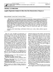
Figure (4.1), (4.2), and (4.3) are the plots of profile relative likelihood of R(β0 ),

R(β1 ), and R(ψ), respectively. These graphs show that the likelihood function is smooth and has a single maximum over the parameter space. The parameter set that maximizes the likelihood function is (βˆ0 = −2.76, βˆ1 = 1.12, ψˆ = 0.32).

4.3.4

Comparison of Model Fitting: the Fixed Effects Logistic Regression Model vs. the Logistic-Normal Regression Model

Data in Table 4.1 is also fitted to the fixed effects logistic regression model by ignoring the random herd effect. The fixed effects model is logit(pij ) = β0 + β1 xij , 28

(4.7)

and the likelihood function is L(β0 , β1 ) =

ni 4 Y Y yij exp(β0 + β1 xij ) . 1 + exp(β + β x ) 0 1 ij i=1 j=1

The model fitting statistics and model parameter estimates using the fixed effect logistic model and the logistic-normal model are listed in Table 4.2. The maximum likelihood estimators for β0 and β1 from the fixed effects logistic model are (βˆ0 = −2.71, βˆ1 = 1.12). They are very close to those from the logistic-normal model. However, the maximum likelihood is smaller in the fixed effects logistic regression model with -2log L being 216.5, compared to 208.2 in the logistic-normal model. The difference in the two models in -2log L was 8.3 with a difference in the model degree of freedom of 1. Since the fixed effect logistic model and the logistic-normal regression model are two types of models, the fixed effects model is not simply the reduced model for the mixed effect model. Therefore, the difference in -2log L does not follow a χ2 distribution with degrees of freedom of 1, in stead it follows a 50:50 mixture of χ21 and χ20 (Pierce and Sands, 1975; Mauritsen, 1984). The probability of observing the likelihood ratio statistic of a value of 8.3 or larger from a χ21 is 0.004, therefore, the p-value of testing no random effect (i.e, variance of the random effect is 0) is at most 0.004. So we can say that the logistic-normal model fits the data better than the fixed effect logistic model at alpha level of 0.01. TABLE 4.2. Comparison of the log-likelihood and parameter estimates for a logistic-normal regression model (LNM) and a fixed effects logistic regression model (FEM).

−2LogL Model D.f. βˆ0 βˆ1 ψˆ

FEM LNM 216.5 208.2 2 3 −2.71 −2.75 1.12 1.10 0.35

29

FIGURE 4.1. The profile relative likelihood R(β0 ) for a logistic-normal regression model.

FIGURE 4.2. The profile relative likelihood R(β1 ) for a logistic-normal regression model.

30

FIGURE 4.3. The profile relative likelihood R(ψ) for a logistic-normal regression model.

31

Chapter 5. Power Analysis for the Logistic-Normal Regression Model 5.1

Introduction

Logistic regression models with random effects have been used frequently in veterinary epidemiological studies to analyze clustered binary data. There are several models that have been developed since the 1980s. The beta-binomial model, introduced by Williams (1982) for identical independent distributed (iid) responses or exchangeable responses within a cluster, assumes that the binomial parameter follows a beta distribution. The logistic-normal model (Stiratelli et al., 1984; Anderson and Aitkin, 1985) assumes a normal or multivariate normal distribution of the parameters corresponding to the random covariates. This model allows the covariates within a cluster to vary, which makes it applicable to broader study designs and is applicable to both exchangeable and non-exchangeable responses. The logistic-binomial model introduced by Mauritsen (1984) is similar to the logistic-normal model except it assumes that the model parameter follows a binomial distribution. When the total events of the prior binomial distribution gets large, this model converges to the logistic-normal model. Another approach to modeling clustered binary data is the Generalized Estimation Equation (GEE) Model introduced by Liang and Zeger (1985), where the dependency or correlation between subjects within the cluster is taken into account by robust estimation of the variance-covariance of the regression coefficients. The GEE model treats the dependency within the cluster as a nuisance. All four models above are being used in veterinary epidemiologic studies. In contrast to the well-developed methods in modeling the clustered binary data, the sample size/power analysis methods corresponding to such models are not very well developed. Several recent papers have described sample size methods for testing one proportion from the clustered binary data (Donner and Eliasziw, 1992; Donner, 1992; Lee and Dubin, 1994; Jung et al., 2001). These methods are not regression modelbased and are applicable to exchangeable responses where subjects within a cluster are

32

exchangeable. More recently, Liu et al. (2002) developed a sample size method for the GEE Models. When using GEE to model the data, misspecification of the ”working correlation” has little effect on model fitting. However, for sample size estimation, the authors pointed out that it is crucial to correctly specify the ”working correlation”. Unfortunately, it is very difficult to do so in the planning stage since very often little is known about the nature of the variance-covariance structure. In this study we propose a power analysis/sample size method for the logisticnormal model described by Stiratelli et al. (1984). The proposed power analysis method extends the sample size method developed by Self et al. (1992) for fixed effects generalized linear models to include random effects. The logistic-normal model and its likelihood function has been described in detail in Chapters 4. In this chapter we will develop a power analysis method for the logistic-normal model where the likelihood ratio test is utilized to make influence on the model parameters.

5.2

Likelihood Decomposition and Expectation

Self et al. (1992) described an approach for sample size/power analysis for the fixed effects generalized linear models based on a noncentral χ2 approximation to the distribution of the likelihood ratio statistics. We adopt their approach and extend it to the logistic-normal regression model with log-likelihood function of (4.4). Let α be the model parameters of interest with dimension p, and φ be the model parameters that are not of interest with dimension q (including the covariance parameter Ψ, which is often treated as nuisance parameter). For testing the null hypothesis of α = α0 , the likelihood ratio statistic can be decomposed into three terms in the way ˆ are maximum likelihood estimates ˆ φ) similar to Self et al. (1992) as in (5.1), where (α, ˆ is the MLE of φ under the null (MLE) of (α, φ) under the alternative model and φ 0 model. φ∗0 is the MLE of φ under the null model when the sample size is very large, ˆ in the paper by Self and Mauritsen which was referred as the limiting value of φ 0 (1988).

33

h i h i ˆ − `n (α , φ ˆ ) = 2 `n (α, ˆ − `n (α, φ) ˆ φ) ˆ 2 `n (α, φ) 0 0 h i ˆ ) − `n (α , φ∗ ) − 2 `n (α0 , φ 0 0 0 £ ¤ + 2 `n (α, φ) − `n (α0 , φ∗0 ) ,

(5.1)

Using asymptotic expansion as in Lawley (1956) (see appendix for details) and taking only the lead term, the approximate expected value for the first term of the tight hand side of the equation in (5.1) is (p + q) and the approximate expected value for the second term is the trace of matrix A, where matrix A is given by ¸· ¸0 ¾ ¸¾−1 ½· ½ · 2 ∂`n (α, φ) ∂`n (α, φ) ∂ `n (α, φ) E − |(α0 ,φ∗0 ) − |(α0 ,φ∗0 ) |(α0 ,φ∗0 ) , E − ∂φ ∂φ ∂φ∂φ0 and the expectations are taken with respect to the true parameters (α, φ). The expectation of the third term in equation (5.1), denoted by ∆, can be calculated exactly in the fixed effects model. In the logistic-normal model with likelihood of (4.3), ∆ can be evaluated numerically. The expectation of `n (α, φ), the first half of the third term in equation (5.1), ignoring the constant of 2, can be expressed as follows ! ( "Z à n ¡ 1 0 −1 ¢ # M i Y X X exp − 2 bi Ψ bi yij p pij (1 − pij )1−yij dbi log k/2 k (2π) |Ψ| R j=1 i=1 all possible yi "Z n ¡ 1 0 −1 ¢ #) i Y y ij 1−yij exp − 2 bi Ψ bi p dbi × . (5.2) pij (1 − pij ) (2π)k/2 |Ψ| Rk j=1

The expectation of `n (α0 , φ∗0 ) also has the above form but the log-likelihood is at

first evaluated at (α0 , φ∗0 ) before the expectation is taken. Evaluating the expectation of `n (α, φ) and `n (α0 , φ∗0 ) with the above form is very tedious when ni are large, which is quite common in veterinary epidemiologic studies. To simplify the evaluation process, we group the categorical covariates into certain number of distinct configurations of covariates (continuous covariates can be grouped into smaller number of categories). Let Ci denote the number of distinct configurations of all possible covariates within the ith cluster. Let πis be the proportion of subjects in 34

cluster i with the sth covariate configuration, where s = 1, 2, . . . , Ci and

PCi

πis = 1. P i yij . Furthermore, let ui be the number of successful events for cluster i, i.e., ui = nj=1 s=1

Now we can use the property of E(Y ) = E (E(Y |X)) to simplify the evaluation of the expectation in (5.2). Let `i be the log-likelihood for cluster i and g(bi ) be the multivariate normal density for bi , we have E(`i ) = E [E (`i |X i )] =

Ci X s=1

{πis × E(`i |X i = X is )} ,

(5.3)

where E(`i |X i = X is ) =

ni µ ¶ X ni

ui =0

×

Z

Rk

ui

log

Z

Rk

puisi (1 − pis )ni −ui g(bi )dbi

puisi (1 − pis )ni −ui g(bi )dbi .

(5.4)

Substituting (5.4) into (5.3), we have ( Z ni µ ¶ Ci X X ni πis log E(`i ) = puisi (1 − pis )ni −ui g(bi )dbi u k i R ui =0 s=1 ¾ Z ui ni −ui g(bi )dbi , pis (1 − pis ) × Rk

and E(`) =

M X

E(`i ).

i=1

Using the above expressions, the expectation in equation (5.2) can be re-expressed as Ci M X X

(

ni µ ¶ X ni

"Z

¢ exp(− 21 b0i Ψ−1 bi ) p dbi πis log puisi (1 − pis )ni −ui k/2 u k (2π) |Ψ| i R ui =0 i=1 s=1 "Z #) 1 0 −1 ¡ ui ¢ exp(− Ψ b ) b i i 2 p pis (1 − pis )ni −ui dbi × . (2π)k/2 |Ψ| Rk ¡

# (5.5)

Calculation of E [`(α0 , φ∗0 )] is similar to the above but pis is evaluated at (α0 , φ∗0 ). Despite its complicated appearance, the expectation in (5.5) is not very difficult to evaluate if the number of distinct covariate configurations is small at the planning 35

stage, which is true for most studies. The expectation for the entire third term of 5.1 is: ∆ = 2

Ci M X X

"Z

i=1 s=1

(

πis

ni µ ¶ X ni

ui =0

ui

log

"Z

exp(− 12 b0i Ψ−1 bi ) p dbi puisi (1 − pis )ni −ui (2π)k/2 |Ψ| Rk

#)

#

1 0 −1 ui ni −ui exp(− 2 bi Ψ bi ) p × pis (1 − pis) dbi |(α,φ) k/2 (2π) |Ψ| Rk ( "Z # Ci ni µ ¶ M X 1 0 −1 X X exp(− b Ψ b ) ni i 2 i p puisi (1 − pis )ni −ui −2 πis dbi log k/2 u k (2π) |Ψ| i R u =0 i=1 s=1

×

5.3

"Z

Rk

i

puisi (1 −

1 0 −1 ni −ui exp(− 2 bi Ψ bi ) p dbi pis) k/2 (2π) |Ψ|

#)

|(α0,φ∗0). (5.6)

Power Determination h

i ˆ ˆ ˆ φ) − `n (α0 , φ0 ) under the alternative hypothesis can The distribution of 2 `n (α,

be approximated by the noncentral χ2 distribution with p degrees of freedom and nonh i ˆ ˆ ˆ φ) − `n (α0 , φ0 ) centrality parameter of γ (Self et al., 1992). Thus the expectation of 2 `n (α,

is approximately (p + γ). Equating this to the approximation of the right hand-side terms of (5.1) derived above yields p + γ = (p + q) − Tr(A) + ∆,

(5.7)

γ = [q − Tr(A)] + ∆.

(5.8)

or

For a given covariate configuration and planning values for (α, Ψ), we can approximate the power of the likelihood ratio test by computing γ and then referring to non-central χ2p tables for the probability of exceeding the critical value. The sample size formula can not be easily obtained from equation (5.8) since the ni can not be factored out from the equation. However, the sample size can be obtained from the power curve generated from formula (5.8). 36

Chapter 6. Examples of Power Analysis for the Logistic-Normal Model For a wide range of parameter values and other planning values, we can construct the power curve using the power analysis method described in Chapter 5. To illustrate how to use the power method we present a couple of examples in this chapter. Prior information about the parameters and planning values were derived from analyzing the example data drawn from a large animal health database provided by Dr. ´ Emile Bouchard and Dr. Denis Du Tremblay, DS@HR, Faculty of Veterinary Medicine, University of Montreal. The sub-dataset included herds that have at least one year of validated mastitis data as of January 1st , 2000 and followed up for at least one year after January 1st , 2000. Only cows that calved in 1999 were included. The sub-dataset consists of 329 herds and 22775 lactations. Variables included are cow identification number, herd identification number and herd size, mastitis status during lactation, number of previous lactations, and culling status. The response variable of interest is culling during the current lactation period (coded as 1 for being culled and 0 for not being culled). The fixed effect explanatory variables are mastitis during lactation (coded as 1 for having developed mastitis and 0 for no mastitis) and the number of previous lactations (coded as 0 for ≤ 3 lactations and 1 for > 3 lactations). For simplicity, herd effect is considered as a random effect on intercept only. In other words, the baseline culling probability varies across herds but the effect of either mastitis status or number of previous lactation on culling is the same across all herds. We will use two examples to illustrate the usage of the power analysis method to determine the power of likelihood ratio test for a given sample size or the minimum required sample size to achieve certain power. There are several ways of sampling from the study population. Two common ways are equal size sampling, i.e., the same number of subjects are sampled from each cluster, and equal proportion sampling, i.e., the number of subjects sampled from each cluster is proportional to the total number of subjects in that herd. For simplicity, we use the

37

equal size sampling in these examples. The other ways of sampling can be incorporated into the power analysis method easily.

6.1 6.1.1

Example 1: A Logistic-Normal Model With One Fixed Effect and One Random Effect The Model and Its Likelihood Function

In this example, we only consider the mastitis effect on culling for illustration purposes. Let y i denote an ni -vector of culling status for the ith cluster, i = 1, 2, . . . , M , each element yij is assumed to be a binary response, and xi is an ni -vector covariate of mastitis status. Let β0 be the regression coefficient for the intercept, β1 be the coefficient for mastitis effect, and bi be the random cluster effect on β0 which is assumed to be normally distributed with a mean of 0 and a variance of ψ 2 . The model is: logit(pij ) = β0 + β1 xij + bi ,

(6.1)

where pij = Pr(yij = 1) is the probability of the jth cow in the ith herd being culled. In epidemiology, researchers are more familiar with p0 , the baseline culling rate, and Odds Ratio for these terms are practically more meaningful to them. The relationship between regression model parameters (β0 , β1 ) and (p0 , OR) are following: exp(β0 ) p0 , or β0 = log( ) 1 + exp(β0 ) 1 − p0 p1 1−p OR = exp(β1 ) = p0 1 . 1 − p0 p0 =

The likelihood function for given data in terms of regression coefficient is µ ¶ ni 4 Z Y Y b2i exp(β0 + bi + β1 xij )yij 1 −1/2 exp − 2 dbi . L(β0 , β1 , ψ) = (2π) 1 + exp(β0 + bi + β1 xij ) ψ 2ψ i=1 R j=1

(6.2)

6.1.2

Hypothesis Testing and Planning Values

The hypothesis being tested using the likelihood ratio test is H0 : β1 = 0. β0 and ψ 2 are considered as nuisance parameters. The parameter estimates derived from d = 1.14, ψˆ = 0.10). The fitting the model (6.1) to the example data are (ˆ p0 = 0.31, OR 38

estimated prevalence of mastitis is 0.2 and the average herd size is 65 cows. Therefore, we use the following plan values to generate power curves: p0 : 0.1 to 0.9 by 0.05 OR : 0.5 to 4 by 0.5 π : 0.1 to 0.7 by 0.05 ψ : 0.1 to 5 by 0.05 The estimates of β0∗ and ψ ∗ are also needed for calculation of the power. In order to obtain β0∗ and ψ ∗ , a pseudo dataset is generated for each combination of (β0 , β1 , ψ, π) with the number of cows per herd 5000 and the number of herds 1000. βˆ0∗ and ψˆ∗ are the estimates of β0 and ψ, respectively, by fitting this pseudo-data with the logistic-normal model under null hypothesis.

6.1.3

Power Analysis

Another issue that needs to be specified is the sampling scheme from the study population. There are several different ways to sample from the study population. Two commonly used sampling schemes are: 1. Equal size sampling, i.e., the same number of cows are sampled from each herd. 2. Equal proportion sampling, i.e., the number of cows sampled from each herd is proportional to the total number of cows in that herd. One special case for this type of sampling is when the sampling fraction is 1, i.e., all cows within the selected herds are sampled. For different sampling schemes, slightly different approaches need to be considered. For simplicity, we will illustrate the application of the proposed power analysis method under the equal size sampling design. From M herds of cows, n cows from each herd are randomly selected into the study. Therefore the total number of subjects required to achieve the desired power is M × n. In the case of equal size sampling, ni in equation (5.6) are the same for all herds. The power for a given sample size n can be approximately calculated using formula (5.8). Calculation of tr(A) can be tedious. Self et al. (1992) and Shieh (2000) demonstrated that the term [q − tr(A)] is very close to zero in the generalized linear model, therefore 39

it can be ignored in the power analysis. Since the likelihood decomposition is based on likelihood with a general form, therefore, it is reasonable to assume that such a term is also small and can be ignored for power analysis purposes for the logistic-normal model. Once the term [q − tr(A)] is ignored, the calculation of power can be simplified as γ u ∆.

(6.3)

This simplified method is to be used for the following examples. Now the planning values are set and (βˆ0∗ , ψˆ∗ ) are obtained, power analysis equation (6.3) can be applied to calculate power for a given sample size.

6.1.4

Results

Figure 6.4 is the power curve with respect to the odds ratio for mastitis effect (note the logarithm scale for horizontal axis), which is the effect to be tested against the null hypothesis of no effect. While other planning values are held fixed, the power for a given size is the lowest when OR = 1, i.e., β1 = 0. The power increases when the value of OR is away from 1. Figure 6.5 displays the power curve with respect to p0 , the baseline culling rate for . mastitis negative cows. This power curve has a minimum at p0 = 0.47. Power increases as p0 takes values away from 0.47. Figure 6.6 shows the effect of π on power while other planning values are held fixed. Power is the largest when π is between 0.3 to 0.4. When compared with the impact of OR and p0 on power, the change in π results in slight change in power. Power decreases as ψ 2 gets larger (Figure 6.7). Power decreases at a higher rate when ψ 2 is small and decreases at a lower rate when ψ 2 gets large. The shape somehow resembles an exponential distribution. Due to technical difficulty, the power can not be evaluated when ψ 2 is very small. In this example when ψ 2 is as small as 0.3, the integration in formula (6.3) and (5.6) can not be obtained. The data point at ψ 2 at 0 is the power for the corresponding fixed effects logistic regression model with the same applicable planning values. 40

FIGURE 6.4. Power curve with respect to the log odds ratio of mastitis effect for a logistic-normal model with one fixed effect and one random effect. p0 = 0.3, π = 0.2, ψ 2 = 2, number of herd = 50, animals per herd = 20.

FIGURE 6.5. Power curve with respect to the baseline culling rate (p0 ) for a logistic-normal model with one fixed effect and one random effect. π = 0.2, OR = 1.5, ψ 2 = 2, number of herd = 50, animals per herd = 20.

41

FIGURE 6.6. Power curve with respect to the prevalence of mastitis (π) for a logistic-normal model with one fixed effect and one random effect. p0 = 0.3, OR = 1.5, ψ 2 = 2, number of herd = 50, animals per herd = 20.

FIGURE 6.7. Power curve with respect to the variance of the random herd effect (ψ 2 ) for a logistic-normal model with one fixed effect and one random effect. p0 = 0.3, π = 0.2, OR = 1.5, number of herd = 50, animals per herd = 20.

42

Figure 6.8 and figure 6.9 illustrate how the power changes as the total sample size changes. As it is shown in Figure 6.8 power increases slowly but steadily while the number of cows per herd increases. Figure 6.9 shows that power increases rapidly with the increase of the number of herds. In these two figures one unit increase of either the number of cows per herd or the number of herds is equivalent to the increase of 40 total sample size. These two graphs suggest that power is more sensitive to the change of the number of herds than the change of the number of cows per herd while other planning values are held fixed.

6.2

Example 2: A Logistic-Normal Model with Two Fixed Effects and One Random Effect

We add the number of previous lactations (0 for ≤ 3 lactation, 1 for > 3 lactations) into the logistic-normal model in Example 1 as a confounding factor and the new model is logit(pij ) = β0 + β1 xij + β2 zij + bi ,

(6.4)

where zij is the value for the number of previous lactations (0 for ≤ 3 lactations and 1 for > 3 lactations) and β2 is its regression coefficient. The likelihood function is −1/2

L(β0 , β1 , β2 , ψ) = (2π)

¶ µ ni 4 Z Y Y exp(β0 + bi + β1 xij + β2 zij )yij 1 b2i exp − 2 dbi . 1 + exp(β0 + bi + β1 xij + β2 zij ) ψ 2ψ R i=1

j=1

The hypothesis being tested using likelihood ratio test is the same as Example 1, i.e., H0 : β1 = 0. Thus (β0 , β2 , ψ 2 ) are considered as nuisance parameters. Instead of specifying π for the prevalence of mastitis, we now have to consider the relative frequency of the number of previous lactations simultaneously. According to the estimates from example data from a dairy herd health surveillance system, the proportion of cows without mastitis and with fewer than three lactations (π00 ) is about 0.6, the proportion of cows without mastitis and with more than three lactations (π01 ) is 0.2, and both the proportion of cows with mastitis and with fewer than three lactations (π10 ) and the proportion of cows with mastitis and with more than three lactations (π11 ) are 0.1. We used these estimates as the planning values and applied them to the power 43

FIGURE 6.8. Power curve with respect to the number of cows per herd for a logistic-normal model with one fixed effect and one random effect. p0 = 0.3, π = 0.2, ψ 2 = 2, OR = 1.5, number of herd 40.

FIGURE 6.9. Power curve with respect to the number of herds for a logistic-normal model with one fixed effect and one random effect. p0 = 0.3, π = 0.2, ψ 2 = 2, OR = 1.5, animals per herd 40.

44

formula (6.3). Other planning values were the same as in Example 1 with the addition of OR for the lactation effect (OR2) taking values from 0.5 to 4 by 0.5.

6.2.1

Results

In the logistic-normal model with two fixed effects and one random effect, the effect of the odds ratio for mastitis effect (OR1) on power is similar to that in the previous example: power is the lowest when OR1 is 1 and power increases as OR1 takes values away from 1. The power curve is close to symmetry when the x-axis is in a logarithm scale (Figure 6.10). The effect of the odds ratio for lactation effect (OR2) on power is very different from that of the odds ratio for mastitis: as OR2 gets larger, power decreases rapidly at first but then decreases slowly when OR is greater than 1 (Figure 6.11). The power curve with respect to p0 has the same shape as in Example 1 except . that the lowest power appears at about p0 = 0.45 (Figure 6.12). The power curves with respect to ψ 2 , the number of cows per herd, and the number of herds are similar to the results observed for Example 1 (Figures 6.13, 6.14, 6.15).

6.3

Comparison of the Results with the Fixed Effect Logistic Regression Model

This section compares the power or sample size results derived from the method for the logistic-normal model with one fixed effect and one random effect with those from the method developed by Self et al. (1992) for the fixed effects logistic regression model. We apply the same planning values that are applicable to each model and compare the power from these two methods. The planning values are: π = 0.3, ψ = 1, the number of herds is 50, the number of cows in each herd is 20, and type I error 0.05. Other planning values and the power are presented in Table (6.3). For the same applicable planning values, the logistic-normal regression model has a smaller power than the corresponding fixed effects logistic regression model for a given total sample size, which implies that the logistic-normal regression model requires a larger sample size than the fix-effect logistic regression model to obtain the same power.

45

FIGURE 6.10. Power curve with respect to the log odds ratio of mastitis effect for a logistic-normal model with two fixed effects and one random effect. p0 = 0.3, ψ 2 = 2, OR2 = 1.5, number of herd = 100, animals per herd = 20.

FIGURE 6.11. Power curve with respect to the log odds ratio of the confounding factor for a logistic-normal model with two fixed effects and one random effect. p0 = 0.3, ψ 2 = 2, OR1 = 1.5, number of herd = 100, animals per herd = 20.

46

FIGURE 6.12. Power curve with respect to the baseline culling rate (p0 ) for a logistic-normal model with two fixed effects and one random effect. OR1 = 1.5, OR2 = 1.5, ψ 2 = 2, number of herd = 100, animals per herd = 20.

FIGURE 6.13. Power curve with respect to the variance of the random herd effect (ψ 2 ) for a logistic-normal model with two fixed effects and one random effect. p0 = 0.3, OR1 = 1.5, OR2 = 1.5, number of herd = 100, animals per herd = 20.

47

FIGURE 6.14. Power curve with respect to the number of cows per herd for a logistic-normal model with two fixed effects and one random effect. p0 = 0.3, ψ 2 = 2, OR1 = 1.5, OR2 = 1.5, number of herd 40.

FIGURE 6.15. Power curve with respect to the number of herds for a logistic-normal model with two fixed effects and one random effect. p0 = 0.3, ψ 2 = 2, OR1 = 1.5, OR2 = 1.5, animals per herd 40.

48

TABLE 6.3. Comparisons of the power for a logistic-normal model (LNM) and a fixed effects logistic regression model (FEM). π = 0.2, the number of herds = 40, and cows per herd = 20 (a total sample size of 800).

p0 0.2 0.3 0.2 0.3

Power for LNM OR Power for FEM ——————————— ψ2 = 1 ψ2 = 2 1.5 0.5922 0.3508 0.3219 1.5 0.6870 0.2120 0.1904 2 0.9736 0.4793 0.4377 2 0.9893 0.3950 0.2817

If the sample sizes are determined using the fixed effects logistic regression model at the planning stage, and the data collected afterwards are analyzed using the logistic-normal regression model, the actual power is expected to be lower than what is specified at the planing stage. The magnitude of the differences in power between these two models depends on the planning values. In the example that includes one fixed effect of mastitis effect and one random herd effect, the difference in power is larger for ψ 2 = 2 than for ψ 2 = 1, larger for p0 = 0.3 than for p0 = 0.2, and larger when OR= 2 than for OR= 1.5.

49

Chapter 7. Discussions 7.1

Estimation of the Limiting Value of the Nuisance Parameters in the Logistic-Normal Model

Hypothesis testing for the logistic-normal regression models often involves one or more nuisance parameters. In the two examples given in chapter 5.3, the nuisance parameters are (β0 , ψ 2 ) for the example with one fixed effect and one random effect and (β0 , β2 , ψ 2 ) for the second example with two fixed effects and one random effect. The estimates of these nuisance parameters under null hypotheses with large sample sizes are necessary for calculating the power. These estimates are obtained by simulation, i.e., first generating a pseudo-data with a large sample size (1000 herds and 5000 animals per herd in the examples presented in chapter 5.3), then estimating these nuisance parameters by fitting the data with the logistic-normal model under null hypothesis. Due to the random error associated with the estimates, this process may result in some roughness of the power curve, as seen in figures (6.6), (6.7), (6.10) to (6.13). Such roughness is more evident for Example 2 than for Example 1. Such variation in estimating the nuisance parameters may also explain why the power curve with respect to the odds ratio for mastitis effect is not exactly symmetric. To study to what extent such variation affects the power, power is calculated four times for the same set of planning values for the Example 1, i.e., p0 = 0.3, π = 0.2, OR = 1.5, ψ 2 = 2, the number of herd = 100 and cows per herd = 20. The mean of the calculated power is 0.3508 and the standard deviation is 0.0116. The coefficient of variance (the ratio of the standard deviation and the mean) is 3.3%, indicating that the variation in power calculation is small under the planning values above.

7.2

Power Curves and Planning Values

In Example 2, the power curve with respect to the odds ratio of mastitis effect is not exactly symmetric, which might be due to the variation in estimating the limiting value of the nuisance parameters.

50

The power curve with respect to the odds ratio of the confounding factor, i.e., the number of lactation is different from that with respect to the odds ratio of mastitis. When the odds ratio is less than 1, i.e., more than three lactations is a protective factor for culling, the power increases to a moderate degree as OR2 decreases. In contrast, when OR2 is greater than 1, i.e., more than three lactations is a risk factor for culling, the power decreases slightly as OR2 increases (Figure 6.11). When the variance of the random herd effect increases, or the variation of β0 among herds gets larger, the power decreases rapidly when the value of ψ 2 is small and decreases slowly when ψ 2 gets larger than 3 (Figure 6.13). The data point for ψ 2 at 0 is the power for the corresponding fixed effects logistic regression model with the same applicable planning values. This graph shows that for the same planning values the logistic-normal regression model has lower power than the corresponding fixed effects logistic regression model for a given total sample size (Figure 6.7). The power curve with respect to p0 is bowl-shaped with a minimum of 0.12 when . . p0 = 0.47 or β0 = −0.2 for Example 1 (Figure 6.5). The minimum power is about . 0.21 when p0 = 0.45 for Example 2 with a confounding factor (Figure 6.12). For the fixed effects logistic regression model, one would expect that the minimum power to be achieved when the average prevalence of culling is 0.5 among all cows. Taking Example 1 as the example but ignoring the random herd effect, in order to obtain the average prevalence of 0.5, p0 should satisfy following conditions:    0.5 = πp1 + (1 − π)p0 , p1 p0   / = OR 1 − p1 1 − p0 where the planning values are π = 0.2 and OR = 1.5. The solution for p0 to the above equations is approximately 0.47. For a logistic-normal model with random herd effects, determining the value for p0 that gives the average prevalence of culling of 0.5 for all cows is not simple. However, one may speculate that the value of p0 for the logisticnormal model is somewhat close to the p0 for the fixed effects model when the number

51

of herds are not small. The maximum of power in examples 1 is around 0.47 which is in agreement with what we expect based on the fixed effects logistic regression model. Compared to the effect of p0 and the odds ratio of mastitis and lactation, the change of π has relatively smaller effect on power. The power curve with respect to π is not symmetric either. Power curve with respect to π is the largest when π is between 0.3 and 0.4. Power is the lowest when π is approaching to 1 (Figure 6.6). Figure 6.8, 6.9, 6.14, and 6.15 show that power increases as the total sample size increases, either through the increase of the number of herds or the increase of the number of cows per herd. However, power is more sensitive to the change of the number of herds than the change of the number of cows per herd. Given the same total sample size, power is higher when the number of herds is larger. To maximize the power for a given total number of sample size, one should include more herds with fewer number of animals per herd. When the number of subjects per herd is 1, the logistic-normal model becomes the fixed effects logistic regression model for the random herd effect bi becomes the random error term for each animal under the fixed effects logistic model. Table 7.4 illustrates that the power for a given total sample size is higher for a larger number of herds. TABLE 7.4. Comparisons of the effect of the number of herds and the number of cows per herd on the power for a logistic-normal regression model with one fixed effect and one random effect. π = 0.2, p0 = 0.1, ψ 2 = 2, OR = 1.5.

Number of Herds Cows per Herd 10 20 20 10

Power 0.2029 0.3080

20 40

40 20

0.3918 0.6141

30 40

40 30

0.5413 0.6457

40 50

50 40

0.6757 0.7593

52

7.3

More Than One Random Effect in the Logistic-Normal Model

Although the two examples given in chapter 5.3 include only one random effect, i.e., the random effect is added only to the intercept, this power analysis method can be applied to the logistic-normal models that include more than one random effect. When more than one random effect is included, the evaluation of the term ∆ involves more complicated calculation. Taking the first example of one fixed and one random effect model, we may allow the random herd effect to apply to the mastitis effect too. Let b1i denote the random herd effect on intercept and b2i as the random effect on mastitis effect. The new model has following form logit(pij ) = β0 + b1i + (β1 + b2i )xij ,

(7.1)

where (b1i , b2i ) follow a bivariate normal distribution of BV N (0, Σ). This model does not only allow the baseline probability of culling to vary among herds but also allows the odds ratio of mastitis effect to vary among herds. Theoretically, the logistic-normal models can include more random effects than fixed effects. However, since the random effects are assumed to have a mean of 0, it is common to add extra fixed effects to account for the non-zero location parameters of the random effects. Therefore, practically the logistic-normal models may include as many random effects as fixed effects plus one more random effect for the intercept.

7.4

Comparing Results with the Fixed Effects Logistic Regression Models

Due to the extra-binomial variation in the logistic-normal model, the variance of the response variable is greater than that in the fixed effects logistic regression model. Therefore, one would expect that for a given sample size the power for the logistic-normal model would be somewhat smaller than that for the fixed effects logistic regression model with the same planing values. Table 6.3 confirms what we have expected. The difference in power between these two models is larger when the variance of the random effect is larger. The difference is larger when the baseline culling rate is 53

0.3 than is 0.2 for planning values presented in Table 6.3. Further study is needed to compare the behavior of the power curve for the logistic-normal model and the fixed effects logistic model under different settings of planning values.

7.5

Further Studies

This dissertation introduces a power analysis method for the logistic-normal model and presents a couple of examples to illustrate how the method can be applied to actual studies using the simplified formula and explores certain properties of this power method. There are more topics needing further research.

7.5.1

Evaluation of Tr(A) and Its Effect on Power

Evaluating Tr(A) in power equation 5.8 is intensive even in the fixed effects logistic regression model (a case of the exponential family) (Self et al., 1992; Shieh 2002). It was pointed out that [q −Tr(A)] is small enough to be ignored in the power calculation. In the logistic-normal model, we believe that [q − Tr(A)] is also very small since the method in above mentioned articles is applicable to the likelihood ratio test with general form of likelihood. Nevertheless, how small that term is and to which extent it affects the power of the logistic-normal regression model need to be further investigated.

7.5.2

Simple Ways of Calculating Power for the LogisticNormal Model with Multiple Random Effects

When multiple random effects are included in the logistic-normal regression models, power calculation becomes very tedious for it involves the evaluation of multidimensional integrations as shown in equation (5.6). Shieh (2002) reported that for power analysis of the fixed effect model of exponential family, an inflation factor derived from the correlation coefficients among the fixed effects is applied to the sample size obtained using a single fixed effect logistic regression model to account for the effect of multiple fixed effects on power. This work compares the sample sizes obtained from inflating the sample size from the simple fixed effects logistic regression model with those obtained using the multiple fixed effects logistic regression model and concludes that the results from the former method is very close to that from the latter 54

method. Further study is needed to explore if such simplification can also be applied to the logistic-normal model with multiple random effects and/or multiple fixed effects.

55

References Abed Y, Archambault D. 2000. A viral transmembrane recombinant protein-based enzyme-linked immunosorbent assay for the detection of bovine immunodeficiency virus infection. J Virol Methods. 85(1-2):109-116. Abed Y, St-Laurent G, Zhang H, Jacobs RM, Archambault D. 1999. Development of a Western blot assay for detection of bovine immunodeficiency-like virus using capsid and transmembrane envelope proteins expressed from recombinant baculovirus. Clin Diagn Lab Immunol. 6(2):168-172. Anderson DA and Aitkin M. 1985. Variance component models with binary response: Interviewer variability. J Royal Stat Society, Series B: Methodological. 47: 203210. Bielanski A, Nadin-Davis S, Simard C, Maxwell P, and Algire J. 2001a. Experimental collection and transfer of embryos from bovine immunodeficiency virus (BIV) infected cattle. Theriogenology. 55(2):641-648. Bielanski A, Simar C, Maxwell P, and Nadin-Davis S. 2001b. Bovine immunodeficiency virus in relation to embryos fertilized in vitro. Vet Res Commun. 25(8):663-673. Bonney GE. 1987. Logistic regression for dependent binary observations. Biometrics. 43: 951-973 Carpenter S, Miller LD, Alexandersen S, Whetstone CA, VanDerMaaten MJ, Viuff B, Wannemuehler Y, Miller JM, and Roth JA. 1992. Characterization of early pathogenic effects after experimental infection of calves with bovine immunodeficiency-like virus. J Virol. 66(2):1074-1083. Carpenter S, Vaughn EM, Yang J, Baccam P, Roth JA, Wannemuehler Y. 2000. Antigenic and genetic stability of bovine immunodeficiency virus during longterm persistence in cattle experimentally infected with the BIV(R29) isolate. J Gen Virol. 81(Pt 6):1463-1472. Cavirani S, Donofrio G, Chiocco D, Foni E, Martelli P, Allegri G, Cabassi CS, De Iaco B, and Flammini CF. 1998. Seroprevalence to bovine immunodeficiency virus and lack of association with leukocyte counts in Italian dairy cattle. Prev Vet Med. 37(1-4):147-157. Cho KO, Meas S, Park NY, Kim YH, Lim YK, Endoh D, Lee SI, Ohashi K, Sugimoto C, and Onuma M. 1999. Seroprevalence of bovine immunodeficiency virus in dairy and beef cattle herds in Korea. J Vet Med Sci. 61(5):549-551. Choi SC and Lu IL. 1995. Effect of non-random missing data mechanisms in clinical trials. Stat Med. 14(24):2675-84. Cockerell GL, Jensen WA, Rovnak J, Ennis WH, and Gonda MA. 1992. Seroprevalence of bovine immunodeficiency-like virus and bovine leukemia virus in a dairy cattle herd. Vet Microbiol. 31(2-3):109-16.

56

Cox DR and Hinkley DV. 1974. Theoretical Statistics. London: Chapman Hall. Crowder MJ. 1978. Beta-binomial ANOVA for proportions. Appl. Statist. 27: 34-37 Donner A. 1992. Sample size requirements for stratified cluster randomization designs Stat. Med. 11: 743-750. Donner A and Eliasziw M. 1992. A goodness-of-fit approach to inference procedures for the kappa statistic: Confidence interval construction, significance-testing and sample size estimation. Stat.Med. 11: 1511-1519. Dyke GV and Patterson HD. 1952. Analysis of factorial arrangements when the data are proportions. Biometrcs. 8: 1-12. Fairclough DL, Peterson HF, and Chang V. 1998. Why are missing quality of life data a problem in clinical trials of cancer therapy? Stat Med. 17(5-7):667-77. Gonda MA. 1992. Bovine immunodeficiency virus. AIDS. 6: 759-776. Gonda MA, Braun MJ, Carter SG, Kost TA, Bess JW Jr, Arthur LO, Van der Maaten MJ. 1987. Characterization and molecular cloning of a bovine lentivirus related to human immunodeficiency virus. Nature. 1987. 330(6146):388-91. Gonda MA, Luther DG, Fong SE, and Tobin GJ. 1994. Bovine immunodeficiency virus: molecular biology and virus-host interactions. Virus Res. 32:155-181 Griffiths DA. 1973. Maximum likelihood estimation for the beta-binomial distribution and an application to the household distribution of the total number of cases of a disease. Biometrics. 29: 37-48. Grimes DA and Schulz KF. 2002. Bias and causal associations in observational research. Lancet. 359(9302):248-52. Horzinek M, Keldermans L, Stuurman T, Black J, Herrewegh A, Sillekens P, and Koolen M. 1991. Bovine immunodeficiency virus: immunochemical characterization and serological survey. J Gen Virol. 72 ( Pt 12):2923-2928. Isaacson JA, Flaming KP, and Roth JA. 1998. Effects of long-term infection with bovine immunodeficiency virus and/or bovine leukemia virus on antibody and lymphocyte proliferative responses in cattle. Vet Immunol Immunopathol. 64(3): 249-266. Jacobs RM, Pollari FL, McNab WB, Jefferson B. Related 1995. A serological survey of bovine syncytial virus in Ontario: associations with bovine leukemia and immunodeficiency-like viruses, production records, and management practices. Can J Vet Res. 59(4):271-278. Jung SH, Kang, SH and Ahn C. 2001. Sample size calculations for clustered binary data Stat.Med. 20: 1971-1982. Kim MY, Goldberg JD. 2001. The effects of outcome misclassification and measurement error on the design and analysis of therapeutic equivalence trials. Stat Med. 20(14):2065-2078. 57

Korn EL and Whittemore AS. 1979. Methods for analyzing panel studies of acute health effects of air pollution. Biometrics. 35: 795-804. Laird N and Ware J. 1982. Random effects models for longitudinal data. Biometrics. 38: 963-974. Lawley DN. 1956. A general method for approximating to the distribution of likelihoodratio criteria. Biometrika. 43: 295-303. Lee EW and Dubin N. 1994. Estimation and sample size considerations for clustered binary responses. Stat.Med. 13: 1241-1252. Liang KY and Zeger SL. 1986. Longitudinal data analysis using generalized linear models. Biometrika. 73(1): 13-22 Liu A, Shih WJ and Gehan E. 2002. Sample size and power determination for clustered repeated measurements. Statistics in Medicine. 21:1787-1801. Liu XH and Liang KY. 1991. Adjustment for non-differential misclassification error in the generalized linear model. Stat Med. 10(8):1197-1211. Martin SJ, O’Neill TP, Bilello JA, and Eiseman JL. 1991. Lymphocyte transformation abnormalities in bovine immunodeficiency-like virus infected calves. Immunol Lett. 27(2):81-84. Mauritsen RH. 1984. Logistic regression with random effects. PhD thesis. Department of Biostatistics, University of Washington. McNab WB, Jacobs RM, and Smith HE. 1994. A serological survey for bovine immunodeficiency-like virus in Ontario dairy cattle and associations between test results, production records and management practices. Can J Vet Res. 58(1):36-41. Meas S, Kabeya H, Yoshihara S, Ohashi K, Matsuki S, Mikami Y, Sugimoto C, and Onuma M. 1998. Seroprevalence and field isolation of bovine immunodeficiency virus. J Vet Med Sci. 60(11):1195-202. Meas S, Ohashi K, Tum S, Chhin M, Te K, Miura K, Sugimoto C, and Onuma M. 2000a. Seroprevalence of bovine immunodeficiency virus and bovine leukemia virus in draught animals in Cambodia. J Vet Med Sci.62(7):779-781. Meas S, Ruas J, Farias NA, Usui T, Teraoka Y, Mulenga A, Chang KS, Masuda A, Madruga CR, Ohashi K, and Onuma M. 2002a. Seroprevalence and molecular evidence for the presence of bovine immunodeficiency virus in Brazilian cattle. Jpn J Vet Res. 50(1):9-16. Meas S, Seto J, Sugimoto C, Bakhsh M, Riaz M, Sato T, Naeem K, Ohashi K, and Onuma M. 2000b. Infection of bovine immunodeficiency virus and bovine leukemia virus in water buffalo and cattle populations in Pakistan. J Vet Med Sci. 62(3):329-331.

58

Meas S, Usui T, Ohashi K, Sugimoto C, and Onuma M. Related 2002b. Vertical transmission of bovine leukemia virus and bovine immunodeficiency virus in dairy cattle herds. Vet Microbiol.84(3):275-282. Meas S, Yilmaz Z, Usui T, Torun S, Yesilbag K, Ohashi K, and Onuma M. 2003. Evidence of bovine immunodeficiency virus in cattle in Turkey. Jpn J Vet Res. 51(1):3-8. Moody CA, Pharr GT, Murphey J, Hughlett MB, Weaver CC, Nelson PD, and Coats KS. 2000. Confirmation of vertical transmission of bovine immunodeficiency virus in naturally infected dairy cattle using the polymerase chain reaction. J Vet Diagn Invest. 43: 239-252. Munro R, Lysons R, Venables C, Horigan M, Jeffrey M, and Dawson M. 1998. Lymphadenopathy and non-suppurative meningo-encephalitis in calves experimentally infected with bovine immunodeficiency-like virus. J Comparat Pathol. 119: 121-134. Muluneh A. 1994. Seroprevalence of bovine immunodeficiency-virus (BIV) antibodies in the cattle population in Germany. Zentralbl Veterinarmed B. 41(10):679-684. Orr KA, O’Reilly KL, and Scholl DT. 2003. Estimation of sensitivity and specificity of two diagnostics tests for bovine immunodeficiency virus using Bayesian techniques. Prev Vet Med. 61(2):79-89 Pierce DA and Sands BR. 1975. Extra-Bernoulli variation in binary data. Tech. Report No. 46. Department of Statistics, Oregon State University. Pinheiro JC and Bates DM. 1995. Approximations to the log-likelihood function in the nonlinear mixed-effects model. J Computatl and Graph Stat. 4: 12-35. Scholl DT, Truax RE, Baptista JM, Ingawa K, Orr KA, O’Reilly KL, and Jenny BF. 2000. Natural transplacental infection of dairy calves with bovine immunodeficiency virus and estimation of effect on neonatal health. Preventive Veterinary Medicine. 43: 239-252. Self SG and Mauritsen RH. 1988. Power/sample size calculations for generalized linear models. Biometrics. 44: 79-86. Self SG, Mauritsen RH, and Ohara J. 1992. Power calculations for likelihood ratio tests in generalized linear models. Biometrics. 48:31-39 Shieh G. 2000. A comparison of two approaches for power and sample size calculations in logistic regression models. Communicat in Stat.–Simulation. 29(3):763-791 Snider TG, Hoyt PG, Jenny BF, Coats KS, Luther DG, Storts RW, Battles JK, and Gonda MA. 1997. Natural and experimental bovine immunodeficiency virus infection in cattle. Vet. Clin. North Am. Food Anim. Pract. 13(1):151-176.

59

Snider TG, Luther DG, Jenny BF, Hoyt PG, Battles JK, Ennis WH, Balady J, BlasMachado U, Lemarchand TX, and Gonda MA. 1996. Encephalitis, lymphoid tissue depletion and secondary diseases associated with bovine immunodeficiency virus in a dairy herd. Comp Immunol Microbiol Infect Dis. 19(2):117-131. Statistics in Epidemiology Research Corporation. Egret statistical software. Seattle: SERC Inc, 1996. Stiratelli R, Laird N and Ware J. 1984. Random effects models for serial observations with binary responses. Biometrics. 40: 961-971. St. Cyr Coats K, Pruett SB, Nash JW, and Cooper CR. 1994. Bovine immunodeficiency virus: incidence of infection in Mississippi dairy cattle. Vet Microbiol. 42(2-3):181-189 Straub OC and Levy D. 1999. Bovine immunodeficiency virus and analogies with human immunodeficiency virus. Leukemia. Suppl 1:S106-109. Usui T, Meas S, Konnai S, Ohashi K, and Onuma M. 2003. Seroprevalence of bovine immunodeficiency virus and bovine leukemia virus in dairy and beef cattle in hokkaido. J Vet Med Sci. 65(2):287-289. van Amelsvoort LG, Beurskens AJ, Kant I, Swaen GM. 2004. The effect of nonrandom loss to follow-up on group mean estimates in a longitudinal study. Eur J Epidemiol. 19(1):15-23. van Der Maaten MJ, Boothe AD, and Seger CL. 1972. Isolation of a virus from cattle with persistent lymphocytosis. J Natl Cancer Inst. 49: 1649-1657 Williams DA. 1982. Extra-binomial variation in logistic linear models. Applied Statistics. 31:144-148. Zhang S, Troyer DL, Kapil S, Zheng L, Kennedy G, Weiss M, Xue W, Wood C, and Minocha HC. 1997a. Detection of proviral DNA of bovine immunodeficiency virus in bovine tissues by polymerase chain reaction (PCR) and PCR in situ hybridization. Virology. 236: 249-257. Zhang S, Wood C, Xue W, Krukenberg SM, Chen Q, and Minocha HC. 1997b. Immune suppression in calves with bovine immunodeficiency virus. Clin Diagn Lab. Immunol. 4: 232-235 References Not Referred Casella G and Berger RL. 1990. Statistical inference. Wadsworth & Brooks, Pacific Grove, CA. Cohen MP. 1998. Determining sample sizes for surveys with data analyzed by hierarchical linear model. J Official Stat. 14(3):267-275. Meeker WQ and Escobar LA. 1998. Statistical methods for reliability data. John Wiley & Sons, Inc. New York, NY. Pinheiro JC and Bates DM. 2000. Mixed-effects models in S and S-Plus. Springer. New York. 60

Appendix: Approximation to the Expectation of the Likelihood Ratio Statistic A brief description of the method for the approximation to the expectation of the likelihood ratio described by Lawley in an article titled ”A general method for approximating to the distribution of likelihood ratio criteria” (1956) is given as follows. Let L be the logarithm of the likelihood function, which depends on p + q parameters θ1 , θ2 , . . . , θp+q . These parameters are assumed functionally independent. Let’s assume that L and its partial derivatives with respect to the θ0 s satisfy some uniform continuity condition which allows differentiations with respect to the θ0 s to commute with integration over the sample space. Let’s further assume that the second derivatives are of order n, where n is related to the number of observations. Let θr0 denote the true value of θr . The hypothesis to be tested is that θp+1 , θp+2 , . . . , θp+q have specific values 0 0 0 θp+1 , θp+2 , . . . , θp+q . θ1 , θ2 , . . . , θp are unspecified and unknown nuisance parameters.

The likelihood ratio can be written as 2(Lp+q − Lp ), where Lk denotes the maximum likelihood with respect to θ1 , θ2 , . . . , θk and substitute true values for the remaining parameters. We shall use the following notation: lr = ∂L/∂θr , Lrs = ∂ 2 L/∂θr ∂θs , Lrst = ∂ 3 L/∂θr ∂θs ∂θt , etc., λrs = E (Lrs ), λrst = E (Lrss ), etc., lrs = Lrs − λrs , lrst = Lrst − λrst , etc. Let θˆ1 , θˆ2 , . . . , θˆk be the estimates for θ1 , θ2 , . . . , θk to produce Lk . The equations for determining the θˆr may be written as 0 = lr + Lrs xs + 1/2Lrst xst + 1/6Lrstu xstu + . . . (r = 1, 2, . . . , k),

(8.1)

where xs = θˆs − θs , and the usual summation convention is used. All suffice run from 1 to k. The inverse expansion of xr in terms of the lx is found to be xr = −Lrs ls − 1/2arst ls lt − 1/2brs,tu ls lt lu + 1/6crstu ls lt lu + . . . ,

61

(8.2)

where arst = Lrg Lsh Lti Lghi , brs,tu = Lrg Lsh Lti Luj Lvw Lghv Lijw , crstu = Lrg Lsh Lti Luj Lghij , and where Lrs is the inverse matrix of Lrs . Next we write L(k) = L + lr xr + 1/2Lrs xr xs + 1/6Lrst xr xs xt + 1/24Lrstu xr xs xt xu + . . . , which in view of (8.1), is equivalent to L − L(k) = 1/2Lrs xr xs + 1/3Lrst xr xs xt + 1/8Lrstu xr xs xt xu + . . . . Substituting the xr in (8.2) in this, we have 2(L(k) − L) = −Lrs lr ls − 1/3arst lr ls lt − 1/4brs,tu lr ls lt lu + 1/12crstu lr ls lt lu + . . . . Hence, including terms up to fourth degree in the l0 s, 2(L(k) − L) = −λrs lr ls − 1/3αrst lr ls lt + λrt λsu lr ls ltu − 1/4βrs,tu lr ls lt lu + 1/12γrstu lr ls lt lu +λrv αstu lr ls lt luv − 1/3λru λsv λtw lr ls lt luvw − λru λsv λtw lr ls ltu lvw . . . , (8.3) where αrst = λrg λsh λti λghi , βrs,tu = λrg λsh λtiλuj λvw λghv λijw , γrstu = λrg λsh λti λuj λghij , and where λrs is the inverse matrix of λrs . The leading term of (8.3) is −λrs lr ls , which is used to approximate the Tr(A) of the likelihood decomposition discussed in Chapter 5.

62

Vita Yinmei Li was born to Mr. Guoyou Li and Mrs. Hanjiao Zhang in Jiangxi Province, People’s Republic of China. She attended Shuangtang elementary and middle school and Jinxi high school, Jinxi County, Jiangxi Province, China. After graduation from high school, she entered Shanghai Medical University, School of Public Health in 1984 and was awarded a degree of Bachelor of Medicine in July 1990 and a degree of Master of Medicine in July 1993. Upon graduating from medical school, she started working as a physician in the Department of Dermatology, Huanshan Teaching Hospital, Shanghai Medical University, Shanghai, China. In August 1995, she was admitted to Louisiana State University Graduate School’s Interdepartmental Program in Veterinary Medical Sciences through the Department of Epidemiology and Community Health and was awarded a Master degree in veterinary medical sciences in December 1997. Since December 1997, she worked as a research follow at the National Hansen’s Disease Center located at LSU for 4 years. During that time she studied part time in the Department of Experimental Statistics at LSU and was awarded a Master degree in applied statistics in 2002 summer. She is now the Chronic Disease Epidemiologist with the Tennessee State Department of Health. She will receive the degree of Doctor of Philosophy in veterinary medical sciences in May 2006.

63