48

NEW TUNING RULES FOR 2-DOF PI/PID CONTROL SYSTEM USING SIMPLE DESIGN PROCEDURE Dr. Basil H. Jasim. Department of electrical engineering, college of engineering, University of Basrah. Abstract Using simple analytical procedure, a tuning rules for two degree of freedom (2-DOF) PI/PID controllers are presented. The proposed tuning algorithm assumes first order plus delay time and second order plus delay time as plant models to be controlled. The validity and features of the proposed tuning rules have been investigated by computer simulation study. Simulation study showed that the presented controllers have high performance response for step input changes and also that these rules are robust for load disturbance.

-‫قواعد تنغيم جديدة لمتحكمات درجة الحرية الثنائية المكونة من المسيطرات تناسب‬ ‫تفاضل من خالل استخدام اجراء تصميمي بسيط‬-‫تكامل‬-‫تكامل وتناسب‬ .‫ باسل هاني جاسم‬.‫د‬ ،‫ كلية الهندسة‬,‫قسم الهندسة الكهربائية‬ .‫جامعة البصرة‬

:‫الخالصة‬ ‫ لم ل دعم معادنغ لنليم للمديكماغ ااغ اليرعة الينائية المكمنة من المستتي راغ‬,‫من خالل استتداداا اجرات ليليلي بستتيم‬ ‫ طرع ة الدنليم الم سدادمة افدر ضت ان المنظمماغ المراد ال سي رة عليها‬.‫لفا ضل‬-‫لكامل‬-‫لكامل و لنا سب‬-‫من النمع لنا سب‬ ‫ صتتتتتتالاية معادنغ الدنليم وكزلت ميزالها لم‬.‫من نمع الدرجة انولى ااغ الزمن الميت و الدرجة اليانية ااغ الزمن الميت‬ ‫ المياكاة هزه بينت ان معادنغ الدنليم الم دراة لمدلت اسدجابة عالية‬.‫اثبالها من خالل دراسة اسدادمت المياكاة بالياسب‬ ‫الجمدة لدليراغ اندخال الدي لكمن على شتتتتكل خ ماغ وكزلت ان المديكماغ الم دراة لكمن صتتتتلبة لجاه انضتتتت راباغ‬ .‫النالجة من لليراغ اليمل‬

1. Introduction

closed loop transfer functions (T.Fs.) that

For control systems, the degree of

can be adjusted [1]. So, a 2- DOF has

freedom (DOF) is defined as the number of

advantages over a 1- DOF control systems

49 because the control design often a multi-

transient response. By using 1- DOF control

objectives problem [1]. In spite of this fact,

system, we often cannot establish the two

2-DOF did not attract a considerable

control operation satisfactory. These two

attention until recent years. Nowadays, a

requirements can more easier be established

considerable attention has been devoted to

by using 2-DOF systems, where these

these systems [2-4].

controller can be managed to have two

Proportional-Integral-Derivative (PID) controllers are with no doubt the most

separate T.Fs., one for regulatory control operation and the other for servo one.

extensive controllers used in industrial

Control design for PID controllers

control applications. Its simple structure

based on optimization techniques with the

and ease of use and understand are the main

aim of good stability and robustness have

reasons for their success.

received attention in the literature [15,16].

There are many methods for the design

Although, these methods proved their

or tuning of PID controller. The first

effectiveness, however, a great drawbacks

systematic

in

involved with them:- They rely on complex

literature was Ziegler-Nichols [5] tuning

numerical optimization procedures and do

rules which had been presented in 1942.

not provide tuning rules.

tuning

rules

presented

Since then, many other tuning rules have

The popularity of tuning rules over the

been presented. Some of these rules

optimization technique comes from their

consider only the performance of the closed

ease to use and their wide applicability over

loop system [6,7], while other consider its

wide range of processes.

robustness only [8,9]. Also, a combination

Most of the tuning rules presented in

of performance and robustness has been

literature like Ziegler-Nichols, Cohen-coon

considered in other works [10-14].

and others, are based on the low order plus

Two control requirements are often

delay time approximation of the plant

considered in most of the industrial process

model. FOPDT and SOPDT are the most

control

the

commonly models used for this purpose.

regulatory and servo control operation [2].

This is due to the fact that most processes

The regulatory control is the ability of the

can be effectively approximated by these

control system to reject or cancel the effect

two models.

applications.

These

are

of load variations or disturbances. While,

In this work, we adopted simple

servo control is the ability of the controller

procedure to obtain tuning rules for a 2-

to track the set point changes with good

DOF PI/PID control system. Two sets of

50 efficient tuning rules, one for FOPDT and the other for SOPDT have been presented.

𝑇𝑓𝑑 =

𝑃(𝑠)

(6)

1+𝐶𝑦 (𝑠)𝑃(𝑠)

Tfr is the T.F. from set point to system output, in other words it represents the servo

2. Problem formulation

control operation. Tfd is T.F. from load

Fig.1 shows one possible structure for 2-

disturbance to system output, then it should

DOF control systems. d Cr(s) r u ++ +

play as a regulator T.F. of the overall P(s)

-

control system.

y

Our aim is to design or tune the two controllers (Cy and Cr) so that Tfr and Tfd be

Cy(s)

a servo and a regulatory T.Fs. respectively

Fig.1 a 2-DOF control system.

with high performance. For that aim, a

In this figure, P(s) is T.F. of The controlled

simple design procedure have been used to

process, Cr(s) is T.F of the set point

design Cr and Cy as PI and PID controllers

controller T.F., Cy(s) T.F of the feedback

for FOPDT or SOPDT.

controller, r the set point, d is the load disturbance and y is the output of the

3. Design procedure

system.

The T.F. for FOPDT is given by:-

Cr and Cy are PI or PID controller with the following T.Fs.:-

𝑝(𝑠) =

𝐾𝑝 𝑒 −𝑙𝑠

Where 𝐾𝑝 is the process gain, T is the time

-PI controller 1

𝐶(𝑠) = 𝐾𝑐 (1 + 𝑇 𝑠)

(1)

𝑖

constant and 𝑙 is the dead time. The T.F. used for SOPDT is:-

-PID controller 1

𝐶(𝑠) = 𝐾𝑐 (1 + 𝑇 𝑠 + 𝑇𝑑 𝑠) 𝑖

(2)

From Fig.1, The output of the controller 𝑈(𝑠) = 𝐶𝑟 (𝑠). 𝑟(𝑠) − 𝐶𝑦 (𝑠). 𝑦(𝑠)

1+𝐶𝑦 (𝑠)𝑃(𝑠)

𝑟(𝑠) +

𝑃(𝑠) 1+𝐶𝑦

𝑑(𝑠) (𝑠)𝑃(𝑠)

(4)

From Eq.4, the output of the system is a result of two T.Fs., these are:𝐶𝑟 (𝑠)𝑃(𝑠)

𝑇𝑓𝑟 = 1+𝐶

𝑦 (𝑠)𝑃(𝑠)

𝐾𝑝 𝑒 −𝑙𝑠

2𝑠

The

(8)

2 +𝑡 𝑠+1 1

design

procedure

for

the

two

1- Substitute the equations for Cr(s), Cy(s) (3)

The output of the system (Y(s)) is given by:𝐶𝑟 (𝑠)𝑃(𝑠)

𝑝(𝑠) = 𝑡

controllers can be summarized as follow:-

(U(s)) is given by:-

𝑌(𝑠) =

(7)

𝑇𝑠+1

and P(s) into Eq.5 and 6. 2- Propose desired T.Fs. for Tfr and Tfd ‘say Tfrd and Tfdd respectively’. 3- Equate Tfdd with Tfd which result from step 1. Then manipulate the resultant

(5)

equation to obtain a homogeneous

51 polynomial equation with s. Each term

by an algebraic equation. So , design

in

represent

problem will be converted to a problem of

homogeneous equation. The number of

guessing one design parameter which

these equations should be equal to the

determine the desired regulatory behavior.

number of controller (Cy) parameters.

Substituting Eq.7 and 10 into 6 and equating

Now, these equations can be solved

the resulting equation with the desired

simultaneously to obtain controller

regulatory T.F. described by Eq.11, then by

parameters.

some manipulation, the following equation

this

polynomial

4- After the parameters of Cy have been

can be obtained:-

obtained, the procedure described in

𝜎1 𝑠 3 + 𝜎2 𝑠 2 + 𝜎3 𝑠 = 0

step 3 can be applied for Tfrd and Tfr to

Where,

obtain Cr(s) parameters.

𝜎1 = (𝐾𝑦 𝑘𝑐𝑦 𝐾𝑝 𝑙 𝑇𝑖𝑦 − 𝑇𝑖𝑦 (𝐾𝑦 𝑇 − 𝐾𝑝 𝑇 2 𝑡𝑦 2 )) (13)

(12)

𝜎2 = (𝐾𝑦 𝑘𝑐𝑦 𝐾𝑝 𝑙 − 𝑇𝑖𝑦 (𝐾𝑦 − 2 𝐾𝑝 𝑇 𝑡𝑦 ) −

3.1 Controllers design for FOPDT

𝐾𝑦 𝑘𝑐𝑦 𝐾𝑝 𝑇𝑖𝑦 )

(14)

The T.F. for FOPDT model is described by Eq.7. Cr and Cy are selected as a PI

𝜎3 = (𝐾𝑝 𝑇𝑖𝑦 − 𝐾𝑦 𝑘𝑐𝑦 𝐾𝑝 )

controller with the following T.Fs.:-

In this derivation, we have used the Pade

𝐶𝑟 (𝑠) = 𝐾𝑐𝑟 (1 + 𝐶𝑦 (𝑠) = 𝐾𝑐𝑦 (1 + 𝑇

1 𝑖𝑦 𝑠

)

1 ) 𝑇𝑖𝑟 𝑠

first order approximation for time delay:𝑒 −𝑙𝑠 = 1 − 𝑙𝑠 (10)

To find tuning rules for Cy(s), the procedure begins with selecting a desired regulatory T.F. ‘Tfdd’, which has been selected as 𝐾𝑦

𝑇𝑓𝑑𝑑 = (𝑡

2 𝑦 𝑇𝑠+1)

To ensure that Eq.12 is true for all values of S, we should force Eqs.13 to 15 to be equal to zero, and mathematically:𝐾𝑦 𝑘𝑐𝑦 𝐾𝑝 𝑙 𝑇𝑖𝑦 − 𝑇𝑖𝑦 (𝐾𝑦 𝑇 − 𝐾𝑝 𝑇 2 𝑡𝑦 2 ) = 0 𝐾𝑦 𝑘𝑐𝑦 𝐾𝑝 𝑙 − 𝑇𝑖𝑦(𝐾𝑦 − 2 𝐾𝑝 𝑇 𝑡𝑦 ) − 𝐾𝑦 𝑘𝑐𝑦 𝐾𝑝 𝑇𝑖𝑦 = 0

follow:𝑠𝑒 −𝑙𝑠

(15)

(11)

𝐾𝑝 𝑇𝑖𝑦

− 𝐾𝑦 𝑘𝑐𝑦 𝐾𝑝 = 0

(16) (17) (18)

Where, Ky and ty are design parameters. Tfdd is a regulatory T.F. which can be fully

Eqs.16 to 18 contains four unknown

adjusted by their two parameters Ky and ty.

variables, the controller parameters ‘Kcy and

Our design procedure will lead to make one

Tiy’ and the two design parameters ‘Ky and

of these two parameters as an independent

ty’. We solved these equations for Kcy, Tiy

variable, while the other will be dependent

and Ky, leaving ty to be the independent

variable related to the independent variable

52 design parameter to be suitably chosen. The

for Kcr, Tir, and Kr, the following equations

result was the following equations:-

can be obtained:-

𝑘𝑐𝑦 = 𝑇𝑖𝑦 = 𝐾𝑦 =

2 𝑇 2 𝑡𝑦 + 𝑙 𝑇 − 𝑇 2 𝑡𝑦 2 𝐾𝑝 (𝑙 2 + 2 𝑙 𝑇 𝑡𝑦

2 𝑇2

𝑡𝑦 + 𝑙

𝑇− 𝑇 2

𝑡𝑦

+ 𝑇 2 𝑡𝑦 2 )

2

(20)

𝑙+𝑇 𝐾𝑝 (𝑙2 + 2 𝑙 𝑇 𝑡𝑦 + 𝑇 2 𝑡𝑦 2 ) 𝑙+𝑇

(21)

𝐾𝑐𝑟 = 2𝑇

𝜌 𝑖𝑦 (𝑇−

𝑇𝑖𝑟 = 2 𝐾

𝜌

𝐾𝑟 = 2𝑘

𝜌

𝑝 𝑇𝑡𝑦 𝑇𝑖𝑦

(28)

𝑐𝑦 𝐾𝑝 𝑇𝑡𝑦

(29)

Where,

Eqs.19 and 20 represent the tuning rules for

𝜌 = 𝜇 + 𝑇𝑡𝑦 𝑇𝑖𝑦 − 𝑘𝑐𝑦 𝐾𝑝 𝑙𝑡𝑟

Cy, while Eq.21 represents the relationship between

the

desired

regulatory

T.F.

parameters Ky and ty. It is clear that Ky in

+ 𝐾𝐶𝑦 𝐾𝑝 𝑇𝑡𝑟 𝑇𝑖𝑦 In which; 𝜇

Eq.21 do not have to be calculated. Now, to tune Cr(s), the following T.F. for

=

√Tt 𝑟 ( 𝑘𝑐𝑦 2 𝐾𝑝 2 l2 + 2 𝑘𝑐𝑦 2 𝐾𝑝 2 lTiy + 𝑘𝑐𝑦 2 𝐾𝑝 2 Tiy 2 2𝐾𝑝 Tt 𝑟 Tiy

the servo control desired T.F. can be used:𝐾𝑟𝑒 −𝑙𝑠

𝑇𝑓𝑟𝑑 = (𝑡

𝑟 𝑇𝑠+𝐾𝑟)

(27)

𝑘𝑐𝑦 𝐾𝑝 𝑙)

(22)

….

̅̅̅̅̅̅̅̅̅̅̅̅̅̅̅̅̅̅̅̅̅̅̅̅̅̅̅̅̅̅̅̅̅̅̅̅̅̅̅̅̅̅̅̅̅̅̅̅̅̅̅̅̅̅̅̅̅̅̅̅̅̅̅̅̅̅̅̅̅̅̅ − 2 𝑘𝑐𝑦 𝐾𝑝 lTiy + 2 𝑘𝑐𝑦 𝐾𝑝 Tiy 2 − 4T 𝑘𝑐𝑦 𝐾𝑝 Tiy + Tiy 2 )

…

Eq.22 represents a servo T.F. with unity

Eqs.27 and 28 represent the tuning rules for

gain and the speed of response can

Cr, while Eq.29 represents the relationship

determined by the parameter tr.

between the desired servo T.F. parameters

Substituting Eqs.7, 9 and 10 into 5, and

Kr and tr.

simplifying the resultant equation. Then equating the resulting equation with the

3.1 Controllers design for SOPDT

right part of Eq.22. Finally, the following

The same procedure described for FOPDT

equation can be obtained:-

is applied here.

𝜎1 𝑠 3 + 𝜎2 𝑠 2 + 𝜎3 𝑠 = 0

(23)

With, 𝜎1 = 𝐾𝑐𝑟 𝐾𝑝 𝑇𝑡𝑦 𝑇𝑖𝑟 𝑇𝑖𝑦 − 𝐾𝑟 𝑇𝑖𝑟 (𝑇𝑇𝑖𝑦 − 𝐾𝑐𝑦 𝐾𝑝 𝑙 𝑇𝑖𝑦 )

Eq.8. Cr and Cy are selected as a PID (24)

𝜎3 = 𝐾𝑟 𝑘𝑐𝑟 𝐾𝑝 𝑇𝑖𝑦 − 𝐾𝑟 𝑘𝑐𝑦 𝐾𝑝 𝑇𝑖𝑟

controller with the following T.Fs.:𝐶𝑟 (𝑠) = 𝐾𝑐𝑟 (1 +

𝜎2 = 𝐾𝑟 𝑘𝑐𝑟 𝐾𝑝 𝑇𝑖𝑟 𝑇𝑖𝑦 − 𝐾𝑟 𝑇𝑖𝑟 (𝑇𝑖𝑦 − 𝑘𝑐𝑦 𝐾𝑝 𝑙 + 𝑘𝑐𝑦 𝐾𝑝 𝑇𝑖𝑦 )

The T.F. for SOPDT model is described by

𝐶𝑦 (𝑠) = 𝐾𝑐𝑦 (1 + 𝑇 (25) (26)

𝑖𝑦 𝑠

+ 𝑇𝑑𝑦 𝑠)

(31)

To tune Cy(s), the desired regulatory T.F. ‘Tfdd’, has been selected as follow:-

Equating Eqs.24 to 26 to zero and solving the resultant three homogeneous equations

1

1 + 𝑇𝑑𝑟 𝑠) 𝑇𝑖𝑟 𝑠

𝑇𝑓𝑑𝑑 =

𝐾𝑦 𝑠𝑒 −𝑙𝑠 2

(𝑡𝑦 𝑡1 𝑠+1) (𝑡𝑦 𝑡2 𝑠+1)

(32)

53 Where, as before, Ky and ty are design

𝛿3 = 𝐾𝑝 (𝑙3 + 2𝑙 2 𝑡1 𝑡𝑦 + 𝑡2 𝑙 2 𝑡𝑦 + 𝑙𝑡1 2 𝑡𝑦 2 + 2𝑙𝑡1 𝑡2 𝑡𝑦 2 + 𝑡1 2 𝑡2 𝑡𝑦 3 +)

parameters. Substituting Eqs.31 and 8 into 6 and

𝛿4 = 𝑙 2 𝑡2 − 𝑙𝑡1 2 𝑡2 𝑡𝑦 3 + 2𝑙𝑡1 𝑡2 𝑡𝑦

equating the resulting equation with the

− 𝑡1 3 𝑡2 𝑡𝑦 3 + 𝑡1 2 𝑡2 𝑡𝑦 2

desired regulatory T.F. described by Eq.32.

+ 2𝑡1 𝑡2 2 𝑡𝑦 2

The following can be obtained:𝜎1 𝑠 4 + 𝜎2 𝑠 3 + 𝜎3 𝑠 2 + 𝜎4 𝑠 = 0

(33)

In which, 𝜎1 = 𝐾𝑦 𝐾𝑐𝑦 𝐾𝑝 𝑙𝑇𝑑𝑦 𝑇𝑖𝑦 − 𝑇𝑖𝑦 (𝐾𝑦 𝑡2 −

the servo control desired T.F. have been (34)

𝐾𝑝 𝑡1 2 𝑡𝑦 3 ) 𝜎2 = 𝑇𝑖𝑦 (𝐾𝑝 𝑡1 2 𝑡𝑦 2 + 2𝐾𝑝 𝑡1 𝑡2 𝑡𝑦 2 ) +

(35)

𝐾𝑦 𝐾𝑐 𝐾𝑝 𝑙 − 𝐾𝑦 𝐾𝑐 𝐾𝑝 𝑇𝑑𝑦 𝑇𝑖𝑦

selected:𝑇𝑓𝑟𝑑 = (𝑡

𝐾𝑟 𝑒 −𝑙𝑠

𝑟 𝑡2 𝑡1 𝑠+𝐾𝑟)

(42)

Eq.42 represents a servo T.F. with unity

𝜎3 = 𝑇𝑖𝑦 (2𝐾𝑝 𝑡1 𝑡𝑦 − 𝐾𝑦 + 𝐾𝑝 𝑡2 𝑡𝑦 ) +

(36)

𝐾𝑦 𝐾𝑐 𝐾𝑝 𝑙 − 𝐾𝑦 𝐾𝑐 𝐾𝑝𝑇𝑖𝑦 𝜎4 =

Now, to tune Cr(s), the following T.F. for

𝐾𝑝 𝑇𝑖𝑦− 𝐾𝑦 𝐾𝑐𝑦 𝐾𝑝

(37)

gain and the speed of response can determined by the parameter tr. Substituting Eqs.8, 30 and 31 into 5, and

.Now,

Eqs.34 to 37 should all be equal to

zero for Eq.33 to be true. Solving these equations

for

𝐾𝑐𝑦, 𝑇𝑖𝑦 , 𝑇𝑑𝑦 𝑎𝑛𝑑 𝐾𝑦

after

equating them to zero, the following equations

will result:-

simplifying the resultant equation. Then equating the resulting equation with the right part of Eq.42, the following equation can be obtained:𝜎1 𝑠 4 + 𝜎2 𝑠 3 + 𝜎3 𝑠 2 + 𝜎4 𝑠 = 0

(43)

With,

𝛿2

𝐾𝑐𝑦 = 𝛿3

(38)

𝛿2

𝑇𝑖𝑦 = 𝛿1

(39)

𝛿4

𝑇𝑑𝑦 = 𝛿2

(40)

𝛿3

𝐾𝑦 = 𝛿1

(41)

− 𝐾𝑝 𝑙 𝑇𝑑𝑦 𝑇𝑖𝑦 )

(44)

𝜎2 = 𝐾𝑦 𝐾𝑝 𝑇𝑑𝑟 𝑇𝑖𝑟 𝑇𝑖𝑦 − 𝐾𝑦 𝑇𝑖𝑟 (𝑡1 𝑇𝑖𝑦 + 𝐾𝑝 𝑇𝑑𝑦 𝑇𝑖𝑦 − 𝐾𝑐𝑦 𝐾𝑝 𝑙 𝑇𝑖𝑦 )

In these equations:-

+ 𝐾𝑐𝑟 𝐾𝑝 𝑡1 𝑡2 𝑡𝑦 𝑇𝑖𝑟 𝑇𝑖𝑦

𝛿1 = 𝑙 2 + 𝑡1 𝑙 + 𝑡2 2

− 2𝑙𝑡1 𝑡2𝑡𝑦 + 𝑙𝑡1 𝑡2 𝑡𝑦 + 𝑙𝑡2 3

− 𝑡1 𝑡2 𝑡𝑦 + 2𝑡1 𝑡2 𝑡𝑦 + 𝑡2

(45)

𝜎3 = 𝐾𝑦 𝐾𝑐𝑟 𝐾𝑝 𝑇𝑖𝑟 𝑇𝑖𝑦 − 𝐾𝑦 𝑇𝑖𝑟 (𝑇𝑖𝑦 − 𝐾𝑐𝑦 𝐾𝑝 𝑙 +

𝛿2 = 𝑙 2 𝑡1 − 𝑙𝑡1 2 𝑡1 2 𝑡𝑦 2 + 2𝑙𝑡1 2 𝑡𝑦 2

𝜎1 = 𝐾𝑝 𝑡1 𝑡2 𝑡𝑦 𝑇𝑑𝑟 𝑇𝑖𝑟 𝑇𝑖𝑟 − 𝐾𝑦 𝑇𝑖𝑦 (𝑡2 𝑇𝑖𝑦

2

𝐾𝑐𝑦 𝐾𝑝 𝑇𝑖𝑦 ) + 𝐾𝑐𝑟 𝐾𝑝 𝑡1 𝑡2 𝑡𝑦 𝑇𝑖𝑦

(46)

𝜎4 = 𝐾𝑦 𝐾𝑐𝑟 𝐾𝑝 𝑇𝑖𝑦 − 𝐾𝑦 𝐾𝑐𝑦 𝐾𝑝 𝑇𝑖𝑟

(47)

Equating Eqs.44 to 47 to zero and solving the resultant four homogeneous equations

54 for Kcr, Tir, Tdr and Kr, the following

set point and the controlled variable (the

equations can be obtained:-

output) have been assumed in the normal

𝑘𝑐𝑟 = …

𝑇𝑖𝑟 = …

𝐾𝑝 𝑙 𝑇𝑑𝑦 𝛽 2 −𝑡2 𝛽 2 + 𝑡1 𝑡2 𝑡𝑦 𝛽 + 𝐾𝑝 𝑡1 2 𝑡2 2 𝑡𝑦2

operation. These variables are assumed

…

̅̅̅̅̅̅̅̅̅̅̅̅̅̅̅̅̅̅̅̅̅̅̅̅̅̅̅̅̅̅̅̅̅̅̅̅̅̅̅̅̅̅̅̅̅̅̅̅̅ 𝐾𝑝 𝑡1 𝑡2 𝑡𝑦 𝑇𝑑𝑦 𝛽 − 𝐾𝑐𝑦 𝐾𝑝 𝑙 𝑡1 𝑡2 𝑡𝑦 𝛽

(48)

been chosen to have results close to 𝑡1 2 𝑡2 2 𝑡𝑦 𝑇𝑖𝑦 𝛽 − 𝑡2 𝑇𝑖𝑦 𝛽 2 + 𝐾𝑝 𝑙 𝑇𝑑𝑦 𝑇𝑖𝑦 𝛽 2 + 𝐾𝑐𝑟 𝐾𝑝 𝑡1 2 𝑡2 2 𝑡𝑦2

industrial practice situations. …

̅̅̅̅̅̅̅̅̅̅̅̅̅̅̅̅̅̅̅̅̅̅̅̅̅̅̅̅̅̅̅̅̅̅̅̅̅̅̅̅̅̅̅̅̅̅̅̅̅̅̅̅̅̅̅̅ 𝐾𝑝 𝑡1 𝑡2 𝑡𝑦 𝑇𝑑𝑦 𝑇𝑖𝑦 𝛽 − 𝐾𝑐𝑦 𝐾𝑝 𝑙 𝑡1 𝑡2 𝑡𝑦 𝑇𝑖𝑦 𝛽

(49) 𝑇𝑖𝑟 =

close to 70%. All of these assumptions have

4.1 FOPDT The following equation describes the FOPDT chosen for our simulation study:-

𝛽(𝑡2 −𝐾𝑝 𝑙𝑇𝑑𝑦 )

(50)

𝐾𝑝 𝑡1 𝑡2 𝑡𝑦

𝐾𝑦 = 𝛽

(51) Where, β is one of the real roots of z of the following third order polynomial:(𝐾𝑝 𝑙 𝑇𝑑𝑦 𝑇𝑖𝑦 − 𝑡2 𝑇𝑖𝑦 )𝑧

𝑝(𝑠) =

5𝑒 −0.6𝑠 10𝑠 + 1

Selecting ty= tr =0.12 and applying Eq.19,

3

20, 27 and 28, we have Kcy=0.72, Tiy=1.5,

+ (𝐾𝑝 𝑡1 𝑡2 𝑡𝑦 𝑇𝑑𝑦 𝑇𝑖𝑦

Kcr=1.53 , Tir=3.18.

− 𝐾𝑐𝑦 𝐾𝑝 𝑙 𝑡1 𝑡2 𝑡𝑦 𝑇𝑖𝑦

The selection of the independent design

2

+ 𝑡1 𝑡2 𝑡𝑦 𝑇𝑖𝑦 )𝑧

2

2

2

+ ( 𝐾𝑐𝑦 𝐾𝑝 𝑙 𝑡1 𝑡2 𝑡𝑦

parameters ty and tr depends on simple 2

guess which can be obtained by noticing the

− 𝑡1 2 𝑡2 2 𝑡𝑦 2 𝑇𝑖𝑦

desired servo and regulatory T.Fs. which

− 𝐾𝑐𝑦 𝐾𝑝 𝑡1 2 𝑡2 2 𝑡𝑦 2 𝑇𝑖𝑦 )𝑧

are

+ 𝐾𝑐𝑦 𝐾𝑝 𝑡1 3 𝑡2 3 𝑡𝑦 3 = 0

respectively. From these equations the

described

by

Eqs.11

and

22

designer can easily predict that the suitable Eqs.48 to 50 represent the tuning rules for

values of ty and tr depend mainly on the

Cr, while Eq.51 represents the relationship

time constant of the process model T,

between the desired servo T.F. parameters

because the time constant for desired servo

Kr and tr.

and regulatory T.Fs. are tyT and trT respectively. Then, for larger T smaller ty

4. Simulation study

and tr should be selected and vice versa. The

In this section, the tuning rules presented in

process of guessing ty and tr ‘which can be

this paper are applied to control two

selected as the same value’ may be need for

randomly selected FOPDT and SOPDT

some trial and error process to obtain

models. 0 to 100% normalized range for the

perfect values.

55 To investigate the performance of the

100

presented tuning rules, the system has been

90 80

simulated by using Simulink tool of Matlab

70 60

for 50 seconds, zero initial condition was

50

assumed, then a step input of 70% has been

40 30

applied at the beginning of simulation to

20

reach the normal operation (70%), then at

10 0

second 20, an 20% step change has accrued, a load disturbance of 10% has been applied at the second 30 and continues applied till

0

10

20 30 Time (sec)

40

50

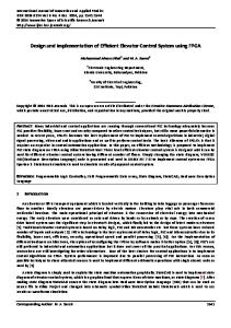
Fig.2 The output of the FOPDT system for the 50 seconds of simulation

the end, then at the second 40 the set point 70

have returned to normal operation.

60

Fig.2 shows the output of the controlled

50

system during the simulated 50 seconds, 40

while Fig.3 shows the output during the first

30

10 seconds.

20

10

4.2 SOPDT

0

2

4

6

8

10

Time (sec)

The SOPDT model used is described by the

Fig.3 The output for FOPDT model for the first 10 seconds of simulation 80

following equation:-

100

−0.5𝑠

𝑝(𝑠) =

0

7𝑒 2 5𝑠 + 10𝑠 + 1

Choosing ty= tr =0.15 and applying the tuning rules described by equations 38 to 40

60

90 80 70

40

60 50

20

40

and 48 to 50, we get Kcy=0.43, Tiy=0.92, Tdy=0.24 Kcr=1.47 , Tir=3.19, Tdy=0.43.

30

0

20

0

2

10

We have simulated the system for 50

0

0

5

4 6 Time (sec) 15 20 25

10

8 30

35

10 40

45

50

Time (sec.)

seconds also and for the same events

80

70

described for the previous case. 60

Fig.4 shows the output of the system for all time of simulation, while Fig.5 shows the

Fig.450 The output SOPDT for the 50 minutes of simulation 40 30

output for the first 10 seconds.

20

10

0

0

1

2

3

4

5 Time (sec.)

6

7

8

9

10

56 70

2- The proposed tuning rules for both

60

FOPDT and SOPDT give excellent

50

transient response for step inputs

40

changes, where they give fast and

30

negligibly overshoot. Also, they give

20

perfect steady state error. 3- The proposed tuning rules give very

10

0

0

2

4

6

8

good for response for load disturbance,

10

Time (sec)

where cancelation of load change has Fig.5 The output SOPDT for the first 10 minutes of simulation

been taken place in relatively small time. Extending the design procedure for more

5. Conclusion

general models is our suggestion for future

A new and not difficult to apply tuning rules

works.

for

6. References

2-DOF

PI/PID

controllers

have

proposed. The procedure used to design

[1] M. Araki and H. Taguchi, “Two-degree-

these

of-freedom PID controllers”, International

tuning

rules

is

simple

and

straightforward, however it needs for some hard manipulation. FOPDT and SOPDT models

which

extensively

used

to

approximate high order plants by low order with input delay are the two models used as controlled plants models for the proposed tuning rules. Simulation study assuming circumstances similar to that faced in industrial conditions has been made. All of the targets for simulation study have been obtained, and as demonstrated through the following points:1- The proposed tuning rules are valid and easy to apply to obtain the controller parameters

Journal

of

Control,

Automation

and

systems, Vol. 1, No. 4, December 2003, pp. 401-411. [2] V. M. Alfaro, “Analytical robust tuning of two-degree-of-freedom PI and PID controllers (ART2)”, Universidad de Costa Rica, September 20, 42 pp., 2007. [3] H.S. Ramadan, H. Siguerdidjane, M. Petit a, R. Kaczmarek, “Performance enhancement and robustness assessment of VSC–HVDC

transmission

systems

controllers under uncertainties”, Electrical Power and Energy Systems 35 (2012) 34– 46. [4] M. Vviteckova and A. Vitecek, “ 2DOF PI and PID controllers tuning”, Proc. 9th

57 IFAC Workshop on Time Delay systems

[11] W.K. Ho, K.L. Lim, C.C. Hang, L.Y.

(TDS) , (6 pp. on CD), Prague, Czech

Ni, “Getting more phase margin and

Republic, June 7-9, 2010.

performance out of PID controllers”,

[5] M. Ramasamya, S. Sundaramoorthy

Automatica 35 (1999) 1579–1585.

“PID controller tuning for desired closed-

[12] A. Ingimundarson, T. Hagglund, K. A˚

loop responses for SISO systems using

strom,

impulse

controllers”, in: 2nd IFAC Conference

response”,

Computers

and

“Criteria

design

PID

Control

1788

Bratislava, Slovak Republic, 2003.

[6] S. Tavakoli, M. Tavakoli, “Optimal

[13] R. Vilanova, “IMC based robust PID

tuning of pid controllers for first order plus

design: tuning guidelines and automatic

time delay models using dimensional

tuning”, Journal of Process Control 18

analysis”,

(2008) 61–70.

Fourth

International

Design

of

Chemical Engineering 32 (2008) 1773–

The

System

for

(CSD’03),

Conference on Control and Automation

[14] Victor M. Alfaroa, Ramon Vilanova,

(ICCA’03), 10-12 June 2003, Montreal,

“Model-reference robust tuning of 2DoF PI

Canada.

controllers for first- and second order plus

[7] O. Eris and S. Kurtulan, “A new pi

dead-time controlled processes”, Journal of

tuning rule for first order plus dead-time

Process Control 22 (2012) 359 374

systems”, IEEE Africon 2011 - The Falls

[15] M. Ge, M. Chiu, and Q. Wang, “Robust

Resort and Conference Centre, Livingstone,

PID Controller design via LMI approach”,

Zambia, 13 - 15 September 2011.

Journal of Process Control, vol. 12, pp. 3

[8] J. Q. Zhou, D. E. Claridge, “PI tuning

13, 2002.

and robustness analysis for air handler

[16] R. Toscano, “A simple PI/PID

discharge air temperature Control”, Energy

controller design method via numerical

and Buildings 44 (2012) 1–6.

optimization approach”, Journal of Process

[9] W.-K. Ho, C.-C. Hang, L.S. Cao,

Control, vol. 15, pp. 81–88, 2005.

“Tuning PID controllers based on Gain and phase margin specifications”, Automatica 31 (3) (1995) 497–502. [10] A.A. Voda, L.D. Landau, “A method for the auto-calibration of PID controllers”, Automatica 31 (1) (1995) 41–53.