*ram* D:/Thomson_Learning_Projects/Brigham_Full_120614/z_production/z_3B2_3D_files/Brigham_0324597703_Ch.10.3d, 12/9/8, 13:52, page: 305

PROPERTY OF CENGAGE LEARNING

PART 4

CHAPTER

INVESTING IN LONG-TERM ASSETS: CAPITAL BUDGETING 10 The Cost of Capital 11 The Basics of Capital Budgeting 12 Cash Flow Estimation and Risk Analysis 13 Real Options and Other Topics in Capital Budgeting

*ram* D:/Thomson_Learning_Projects/Brigham_Full_120614/z_production/z_3B2_3D_files/Brigham_0324597703_Ch.10.3d, 12/9/8, 13:52, page: 306

ª STAN HONDA/AFP/GETTY IMAGES

PROPERTY OF CENGAGE LEARNING

10 The Cost of Capital

General Electric

CHAPTER

Creating Value at GE

General Electric (GE) is one of the world’s bestmanaged companies, and it has rewarded its shareholders with outstanding returns. GE creates shareholder value by investing in assets that earn more than the cost of the capital used to acquire them. For example, if a project earns 20% but the capital invested in it costs only 10%, taking on the project will increase the firm’s value and thus its stock price. Capital is obtained in three primary forms: debt, preferred stock, and common equity, with equity acquired by retaining earnings and by the issuance of new stock. The investors who provide capital to GE expect to earn at least their required rate of return on that capital, and the required return represents the firm’s cost of capital.1 A variety of factors influence the cost of capital. Some—including interest rates, state

and federal tax policies, and general economic conditions—are outside the firm’s control. However, the firm’s decisions regarding how it raises capital and how it invests those funds also have a profound effect on its cost of capital. Estimating the cost of capital for a company such as GE is conceptually straightforward. GE’s capital comes largely from debt plus common equity obtained by retaining earnings, so its cost of capital depends largely on the level of interest rates in the economy and the marginal stockholder’s required rate of return on equity. However, GE operates many different divisions throughout the world; so the corporation is similar to a portfolio that contains a number of different stocks, each with a different risk. Recall that portfolio risk is a weighted average of the relevant risks of the different stocks in the portfolio.

1 Recall from earlier chapters that expected and required returns as seen by the marginal investor must be equal; otherwise, the security will not be in equilibrium. Therefore, buying and selling will force this equality to hold, except for short periods immediately following the release of new information. Since expected and required returns are normally equal, we use the two terms interchangeably.

306

*ram* D:/Thomson_Learning_Projects/Brigham_Full_120614/z_production/z_3B2_3D_files/Brigham_0324597703_Ch.10.3d, 12/9/8, 13:52, page: 307

PROPERTY OF CENGAGE LEARNING Chapter 10 The Cost of Capital

Similarly, each of GE’s divisions has its own level of risk (hence, its own cost of capital). GE’s overall cost of capital is an average of its divisions’ costs. For example, GE’s NBC subsidiary probably has a different cost of capital than its aircraft engine division; and even within divisions, some projects are riskier than others. Moreover, overseas projects

may have different risks and thus different costs of capital than similar domestic projects. As we will see in this chapter, the cost of capital is an essential element in the capital budgeting process. This process is the primary determinant of the firm’s long-run stock price.

PUTTING THINGS IN PERSPECTIVE In the last four chapters, we explained how risk influences prices and required rates of return on bonds and stocks. A firm’s primary objective is to maximize its shareholders’ value. The principal way value is increased is by investing in projects that earn more than their cost of capital. In the next two chapters, we will see that a project’s future cash flows can be forecasted and that those cash flows can be discounted to find their present value. Then if the PV of the future cash flows exceeds the project’s cost, the firm’s value will increase if the project is accepted. However, we need a discount rate to find the PV of the future cash flows, and that discount rate is the firm’s cost of capital. Finding the cost of the capital required to take on new projects is the primary focus of this chapter.2 Most formulas used in this chapter were developed earlier, when we examined the required rates of return on bonds and stocks. Indeed, the rates of return that investors require on bonds and stocks represent the costs of those securities to the firm. As we shall see, companies estimate the required returns on their securities, calculate a weighted average of the costs of their different types of capital, and use this average cost for capital budgeting purposes. When you finish this chapter, you should be able to: Explain why the weighted average cost of capital (WACC) is used in capital budgeting. Estimate the costs of different capital components—debt, preferred stock, retained earnings, and common stock. Combine the different component costs to determine the firm’s WACC. These concepts are necessary to understand the firm’s capital budgeting process. l

l

l

10-1 AN OVERVIEW OF THE WEIGHTED AVERAGE COST OF CAPITAL (WACC) Table 10-1 shows Allied Food Products’ balance sheet as presented in Chapter 3, with two additions: (1) the actual capital supplied by investors (banks, bondholders, and stockholders) and (2) the capital structure that Allied plans to use in the future. Allied’s overall cost of capital is an average of the costs of the various types of capital it uses. Allied’s debt costs 10%, it currently uses no preferred stock

2

307

If projects differ in risk, risk-adjusted costs of capital should be used, not one single corporate cost of capital. We discuss this point later in the chapter.

*ram* D:/Thomson_Learning_Projects/Brigham_Full_120614/z_production/z_3B2_3D_files/Brigham_0324597703_Ch.10.3d, 12/9/8, 13:52, page: 308

PROPERTY OF CENGAGE LEARNING

308

Part 4 Investing in Long-Term Assets: Capital Budgeting

Table 10-1

Allied Food Products: Capital Structure Used to Calculate the WACC

REGULAR BALANCE SHEET: at 12/31/08 Cash $ 10 Accounts payable Receivables 375 Accruals Inventories 615 Spontaneous debt Total C.A. $1,000 Notes payable Total C.L. Net fixed assets $1,000 Long-term debt Total debt Preferred stock Common stock Retained earnings Total equity Total $2,000 Total

All Liabilities & Equity $ 60 3.0% 140 7.0 $ 200 10.0% 110 5.5 $ 310 15.5% 750 37.5 $1,060 53.0% 0 0.0 130 6.5 810 40.5 $ 940 47.0% $2,000 100.0%

Actual Investor-Supplied Capital

Target Capital Structure

$ 110 750 $ 860 0 130 810 $ 940 $1,800

47.8% 0.0

45.0% 2.0

52.2 100.0%

53.0 100.0%

but plans to use a small amount of preferred in the future, and its common equity costs about 13.5%. (This is the return that stockholders require on the stock.)3 Now assume that Allied has made the decision to finance all of next year’s projects with debt. The argument is sometimes made that the cost of capital for next year’s projects will be 10% because only debt will be used to finance them. However, this position is incorrect. If Allied finances this set of projects with debt, it will be using up some of its future borrowing capacity. As expansion occurs in subsequent years, the firm will at some point have to raise more equity to prevent the debt ratio from getting too high. Our concern is with capital that must be provided by investors—interestbearing debt, preferred stock, and common equity. Accounts payable and accruals increase automatically when capital budgeting projects are taken on, so increases in these items are deducted from projects’ costs. This point is discussed in detail in Chapter 12, but the result is that we are concerned only with investor-supplied capital when we calculate the cost of capital. To illustrate, suppose Allied borrows heavily at 10% during 2009 and, in the process, uses up its capacity to borrow, to finance projects yielding 11%. In 2010, it has new projects available that yield 13% (well above the return on 2009 projects), but it could not accept them because they would have to be financed with 13.5% equity. To avoid this problem, Allied and other firms take a long-run view; and the cost of capital is calculated as a weighted average, or composite, of the various types of funds used over time, regardless of the specific financing used in a given year. We explore the weights in more detail in the capital structure chapter, where we see how the optimal capital structure is estimated. As we will see, there is an optimal capital structure—one where the percentages of debt, preferred stock, and common equity maximize the firm’s value. As shown in the last column of Table 10-1, Allied Foods has concluded that it should use 45% debt, 2% preferred stock, and 53% common equity; and it plans to raise capital in those proportions in

3 We estimate this 13.5% later in the chapter. It differs slightly from the number we found in an earlier chapter. As you will see, there are several ways to estimate rs and those methods generally produce different estimates. Allied concluded that its rs is somewhere in the range of 13% to 14%, and it compromised by using 13.5%. The costs of debt and preferred stock are set by contract, so they can be estimated with relatively little error; but the cost of equity cannot be measured precisely.

*ram* D:/Thomson_Learning_Projects/Brigham_Full_120614/z_production/z_3B2_3D_files/Brigham_0324597703_Ch.10.3d, 12/9/8, 13:52, page: 309

PROPERTY OF CENGAGE LEARNING Chapter 10 The Cost of Capital

309

the future. Therefore, we use those target weights when we calculate Allied’s weighted average cost of capital.

SE

LF TEST

Why should the cost of capital be calculated as a weighted average of the various types of funds that a firm generally uses, not as the cost of the specific type of capital used during a given year? What is the riskiest and thus highest-cost type of capital? least-cost type? Why can’t a firm finance with only the lowest-cost type of capital?

10-2 BASIC DEFINITIONS The investor-supplied items—debt, preferred stock, and common equity—are called capital components. Increases in assets must be financed by increases in these capital components. The cost of each component is called its component cost; for example, Allied can borrow money at 10%, so its component cost of debt is 10%.4 These costs are then combined to form a weighted average cost of capital, which is used in the capital budgeting process. Throughout this chapter, we concentrate on the three major capital components. The following symbols identify the cost and weight of each: rd ¼ interest rate on the firm’s new debt ¼ before-tax component cost of debt. It can be found in several ways, including calculating the yield to maturity on the firm’s currently outstanding bonds. rd(1 – T) ¼ after-tax component cost of debt, where T is the firm’s marginal tax rate. rd(1 – T) is the debt cost used to calculate the weighted average cost of capital. As we shall see, the after-tax cost of debt is lower than its before-tax cost because interest is tax deductible. rp ¼ component cost of preferred stock, found as the yield investors expect to earn on the preferred stock. Preferred dividends are not tax-deductible; hence, the before- and after-tax costs of preferred are equal. rs ¼ component cost of common equity raised by retaining earnings, or internal equity. It is the rs developed in Chapters 8 and 9 and defined there as the rate of return that investors require on a firm’s common stock. Most firms, once they have become well established, obtain all of their new equity as retained earnings; hence, rs is their cost of all new equity. re ¼ component cost of external equity, or common equity raised by issuing new stock. As we will see, re is equal to rs plus a factor that reflects the cost of issuing new stock. Note, though, that established firms such as Allied Foods rarely issue new stock; hence, re is rarely a relevant consideration except for very young, rapidly growing firms.

4 We will see shortly that there is a before-tax and an after-tax cost of debt; for now, it is sufficient to know that 10% is the before-tax component cost of debt. Also, for simplicity, we assume that long- and short-term debt have the same cost; hence, we deal with just one type of debt.

Capital Component One of the types of capital used by firms to raise funds.

*ram* D:/Thomson_Learning_Projects/Brigham_Full_120614/z_production/z_3B2_3D_files/Brigham_0324597703_Ch.10.3d, 12/9/8, 13:52, page: 310

PROPERTY OF CENGAGE LEARNING

310

Part 4 Investing in Long-Term Assets: Capital Budgeting

wd, wp, ws, we ¼ target weights of debt, preferred stock, retained earnings (internal equity), and new common stock (external equity). The weights are the percentages of the different types of capital the firm plans to use when it raises capital in the future. Target weights may differ from actual current weights.5 WACC ¼ the firm’s weighted average, or overall, cost of capital. The target proportions of debt (wd), preferred stock (wp), and common equity (wc), along with the costs of those components, are used to calculate the firm’s weighted average cost of capital, WACC. We assume at this point that all new common equity is raised as retained earnings, as is true for most companies; hence, the cost of common equity is rs.

Weighted Average Cost of Capital (WACC) A weighted average of the component costs of debt, preferred stock, and common equity.

1 10 1 0 10 1 0 10 Cost of % of Cost of % of After-tax % C CB C B CB C B CB B WACC ¼ @ of A@ cost of A þ @preferredA@preferredA þ @commonA@commonA equity equity stock stock debt debt 0

¼

10-1

wd rd ð1
TÞ

þ

w p rp

þ

w c rs

Note that only debt has a tax adjustment factor, (1 – T). As discussed in the next section, this is because interest on debt is tax-deductible but preferred dividends and the returns on common stock (dividends and capital gains) are not. These definitions and concepts are discussed in the remainder of the chapter, using Allied Foods for illustrative purposes. Later in the capital structure chapter, we extend the discussion to show how the optimal mix of securities minimizes the firm’s cost of capital and maximizes its value.

SE

LF TEST

Identify the firm’s three major capital structure components and give their respective component cost and weight symbols. Why might there be two different component costs for common equity? Which one is generally relevant, and for what type of firm is the second one likely to be relevant? If a firm now has a debt ratio of 50% but plans to finance with only 40% debt in the future, what should it use as wd when it calculates its WACC?

10-3 COST OF DEBT, rd(1 – T) Before-Tax Cost of Debt, rd The interest rate the firm must pay on new debt.

The interest rate a firm must pay on its new debt is defined as its before-tax cost of debt, rd. Firms can estimate rd by asking their bankers what it will cost to borrow or by finding the yield to maturity (or yield to call if the debt is likely to be

5 We should also note that the weights could be based on the book values of the capital components or on their market values. The market value of the equity is found by multiplying the stock’s price by the number of shares outstanding. Market value weights are theoretically superior; but accountants show assets on a bookvalue basis, bond rating agencies and security analysts generally focus on book values, and market value weights are quite unstable because stock prices fluctuate widely. If a firm’s book and market values differ widely, the firm may set its target weights as a blend of book and market weights. We will discuss this at greater length in the capital structure chapter; but for now, just take the target weights provided in this chapter as management determined.

*ram* D:/Thomson_Learning_Projects/Brigham_Full_120614/z_production/z_3B2_3D_files/Brigham_0324597703_Ch.10.3d, 12/9/8, 13:52, page: 311

PROPERTY OF CENGAGE LEARNING Chapter 10 The Cost of Capital

called) on their currently outstanding debt (see Chapter 7).6 However, the after-tax cost of debt, rd(1 – T), should be used to calculate the weighted average cost of capital. This is the interest rate on new debt, rd, less the tax savings that result because interest is tax deductible:7 After-tax cost of debt ¼ Interest rate on new debt
Tax savings ¼ rd
rd T ¼ rd ð1
TÞ

10-2

In effect, the government pays part of the cost of debt because interest is tax deductible. Therefore, if Allied can borrow at an interest rate of 10% and its marginal federal-plus-state tax rate is 40%, its after-tax cost of debt will be 6%:8 After-tax cost of debt ¼ rd ð1
TÞ ¼ 10%ð1:0
0:4Þ ¼ 10%ð0:6Þ ¼ 6:0%

We use the after-tax cost of debt in calculating the WACC because we are interested in maximizing the value of the firm’s stock, and the stock price depends on after-tax cash flows. Because we are concerned with after-tax cash flows and because cash flows and rates of return should be calculated on a comparable basis, we adjust the interest rate downward due to debt’s preferential tax treatment. Note that the cost of debt is the interest rate on new debt, not on already outstanding debt. We are interested in the cost of new debt because our primary concern with the cost of capital is its use in capital budgeting decisions. For example, would a new machine earn a return greater than the cost of the capital needed to acquire the machine? The rate at which the firm has borrowed in the past is irrelevant when answering this question because we need to know the cost of new capital.9

SE

LF TEST

Why is the after-tax cost of debt rather than the before-tax cost used to calculate the WACC? Why is the relevant cost of debt the interest rate on new debt, not that on already outstanding, or old, debt? How can the yield to maturity on a firm’s outstanding debt be used to estimate its before-tax cost of debt?

6 If the yield curve is sharply upward- or downward-sloping, the costs of long- and short-term debt will differ. In this case, the firm should calculate an average of its debt costs based on the proportions of long- and short-term debt that it plans to use. 7 If Allied borrowed $100,000 at 10%, it would have to write a check for $10,000 to pay interest charges for a year. However, that $10,000 would be a tax deduction, which at a 40% tax rate would save $4,000 in taxes. 8 Note that in 2008, the federal tax rate for most large corporations is 35%. However, most corporations are also subject to state income taxes; so for illustrative purposes, we assume that the effective federal-plus-state tax rate on marginal income is 40%. 9 Three additional points should also be noted: (1) The tax rate is zero for a firm with losses. Therefore, for a company that does not pay taxes, the cost of debt is not reduced. That is, in Equation 10-2, the tax rate equals zero; so the after-tax cost of debt is equal to the interest rate. (2) Strictly speaking, the after-tax cost of debt should reflect the expected cost of debt, which is very slightly below the promised 10% yield. (3) Allied raises most of its debt from commercial banks and sells bonds directly to financial institutions; but if it sold new bonds through investment bankers, a flotation cost would be incurred. We can adjust for flotation costs by deducting the dollar flotation costs from the issue price (par value) of the bond and calculating an adjusted YTM. If the bonds had a flotation cost of 0.5% (or $5 per $1,000 bond), an annual interest rate of 10%, and a 20-year maturity, the calculated YTM would be 10.06% versus 10.00% with no flotation costs. Because the difference is so small, most firms ignore bond flotation costs.

311

After-Tax Cost of Debt, rd(1 – T) The relevant cost of new debt, taking into account the tax deductibility of interest; used to calculate the WACC.

*ram* D:/Thomson_Learning_Projects/Brigham_Full_120614/z_production/z_3B2_3D_files/Brigham_0324597703_Ch.10.3d, 12/9/8, 13:52, page: 312

PROPERTY OF CENGAGE LEARNING

312

Part 4 Investing in Long-Term Assets: Capital Budgeting

A company has outstanding 20-year non-callable bonds with a face value of $1,000, an 11% annual coupon, and a market price of $1,294.54. If the company was to issue new debt, what would be a reasonable estimate of the interest rate on that debt? If the company’s tax rate is 40%, what is its after-tax cost of debt? (8.0%; 4.8%)

10-4 COST OF PREFERRED STOCK, rp The component cost of preferred stock used to calculate the weighted average cost of capital, rp, is the preferred dividend, Dp, divided by the current price of the preferred stock, Pp.

Cost of Preferred Stock, rp The rate of return investors require on the firm’s preferred stock. rp is calculated as the preferred dividend, Dp , divided by the current price, Pp.

10-3

Component cost of preferred stock ¼ rp ¼

Dp Pp

Allied does not have any preferred stock outstanding, but the company plans to issue some in the future and therefore has included it in its target capital structure. Allied would sell this stock to a few large hedge funds, the stock would have a $10.00 dividend per share, and it would be priced at $97.50 a share. Therefore, Allied’s cost of preferred stock would be 10.3%:10 rp ¼ $10:00=$97:50 ¼ 10:3%

As we can see from Equation 10-3, calculating the cost of preferred stock is easy. This is particularly true for traditional “plain vanilla” preferred that pays a fixed dividend in perpetuity. However, in Chapter 9, we noted that some preferred issues have a specified maturity date and we described how to calculate the expected return on these issues. Also, preferred stock may include an option to convert to common stock, which adds another layer of complexity. We leave these more complicated situations for advanced classes. Finally, note that no tax adjustments are made when calculating rp because preferred dividends, unlike interest on debt, are not tax deductible; so no tax savings are associated with preferred stock.

Is a tax adjustment made to the cost of preferred stock? Why or why not?

SE

LF TEST

A company’s preferred stock currently trades at $80 per share and pays a $6 annual dividend per share. Ignoring flotation costs, what is the firm’s cost of preferred stock? (7.50%)

10-5 THE COST OF RETAINED EARNINGS, rs The costs of debt and preferred stock are based on the returns that investors require on these securities. Similarly, the cost of common equity is based on the rate of return that investors require on the company’s common stock. Note, though, that new common equity is raised in two ways: (1) by retaining some of

10

This preferred stock would be sold directly to a group of hedge funds, so no flotation costs would be incurred. If significant flotation costs were involved, the cost of the preferred should be adjusted upward, as we explain in a later section.

*ram* D:/Thomson_Learning_Projects/Brigham_Full_120614/z_production/z_3B2_3D_files/Brigham_0324597703_Ch.10.3d, 12/9/8, 13:52, page: 313

PROPERTY OF CENGAGE LEARNING Chapter 10 The Cost of Capital

the current year’s earnings and (2) by issuing new common stock.11 We use the symbol rs to designate the cost of retained earnings and re to designate the cost of new common stock, or external equity. Equity raised by issuing stock has a higher cost than equity from retained earnings due to the flotation costs required to sell new common stock. Therefore, once firms get beyond the startup stage, they normally obtain all of their new equity by retaining earnings. Some have argued that retained earnings should be “free” because they represent money that is “left over” after dividends are paid. While it is true that no direct costs are associated with retained earnings, this capital still has a cost, an opportunity cost. The firm’s after-tax earnings belong to its stockholders. Bondholders are compensated by interest payments; preferred stockholders, by preferred dividends. But the net earnings remaining after interest and preferred dividends belong to the common stockholders, and these earnings serve to compensate them for the use of their capital. The managers, who work for the stockholders, can either pay out earnings in the form of dividends or retain earnings for reinvestment in the business. When managers make this decision, they should recognize that there is an opportunity cost involved—stockholders could have received the earnings as dividends and invested this money in other stocks, in bonds, in real estate, or in anything else. Therefore, the firm needs to earn at least as much on any earnings retained as the stockholders could earn on alternative investments of comparable risk. What rate of return can stockholders expect to earn on equivalent-risk investments? First, recall from Chapter 9 that stocks are normally in equilibrium, with expected and required rates of return being equal: ^r s ¼ rs. Thus, Allied’s stockholders expect to be able to earn rs on their money. Therefore, if the firm cannot invest retained earnings to earn at least rs , it should pay those funds to its stockholders and let them invest directly in stocks or other assets that will provide that return. Whereas debt and preferred stocks are contractual obligations whose costs are clearly stated on the contracts, stocks have no comparable stated cost rate. That makes it difficult to measure rs. However, we can employ the techniques developed in Chapters 8 and 9 to produce reasonably good estimates of the cost of equity from retained earnings. To begin, recall that if a stock is in equilibrium, its required rate of return, rs, must be equal to its expected rate of return, r^s . Further, its required return is equal to a risk-free rate, rRF , plus a risk premium, RP, whereas the expected return on the stock is its dividend yield, D1/P0 , plus its expected growth rate, g. Thus, we can write the following equation and estimate rs using the left term, the right term, or both terms: Required rate of return ¼ Expected rate of return rs ¼ rRF þ RP ¼ D1 =P0 þ g ¼ ^r s

10-4

The left term is based on the Capital Asset Pricing Model (CAPM) as discussed in Chapter 8, and the right term is based on the discounted dividend model as developed in Chapter 9. We discuss these two procedures, in addition to one based on the firm’s own cost of debt, in the following sections. 11

The term retained earnings can be interpreted to mean the balance sheet item retained earnings, consisting of all the earnings retained in the business throughout its history or the income statement item addition to retained earnings. The income statement item is relevant in this chapter; for our purpose, retained earnings refers to that part of the current year’s earnings not paid as dividends (hence, available for reinvestment in the business this year). If this is not clear, look back at Allied’s balance sheet shown in Table 3-1 and note that at the end of 2007, Allied had $750 million of retained earnings; but that figure rose to $810 million by the end of 2008. Then look at the 2008 income statement, where you will see that Allied retained $60 million of its 2008 income. This $60 million was the new equity from retained earnings that was used, along with some additional debt, to fund the 2008 capital budgeting projects. Also, you can see from the 2007 and 2008 balance sheets that Allied had $130 million of common stock at the end of both years. This indicates that it did not sell any new common stock to raise capital during 2008.

313

Cost of Retained Earnings, rs The rate of return required by stockholders on a firm’s common stock. Cost of New Common Stock, re The cost of external equity based on the cost of retained earnings but increased for flotation costs.

*ram* D:/Thomson_Learning_Projects/Brigham_Full_120614/z_production/z_3B2_3D_files/Brigham_0324597703_Ch.10.3d, 12/9/8, 13:52, page: 314

PROPERTY OF CENGAGE LEARNING

314

Part 4 Investing in Long-Term Assets: Capital Budgeting

10-5a The CAPM Approach The most widely used method for estimating the cost of common equity is the Capital Asset Pricing Model (CAPM) as developed in Chapter 8.12 Here are the steps used to find rs: Step 1: Estimate the risk-free rate, rRF . We generally use the 10-year Treasury bond rate as the measure of the risk-free rate, but some analysts use the short-term Treasury bill rate. Step 2: Estimate the stock’s beta coefficient, bi, and use it as an index of the stock’s risk. The i signifies the ith company’s beta. Step 3: Estimate the expected market risk premium. Recall that the market risk premium is the difference between the return that investors require on an average stock and the risk-free rate.13 Step 4: Substitute the preceding values in the CAPM equation to estimate the required rate of return on the stock in question: 10-5

rs ¼ rRF þ ðRPM Þbi ¼ rRF þ ðrM
rRF Þbi

Thus, the CAPM estimate of rs is equal to the risk-free rate, rRF , plus a risk premium that is equal to the risk premium on an average stock, (rM – rRF), scaled up or down to reflect the particular stock’s risk as measured by its beta coefficient. Assume that in today’s market, rRF ¼ 5.6%, the market risk premium is RPM ¼ 5.0%, and Allied’s beta is 1.48. Using the CAPM approach, Allied’s cost of equity is estimated to be 13.0%: rs ¼ 5:6% þ ð5:0%Þð1:48Þ ¼ 13:0%

Although the CAPM appears to produce an accurate, precise estimate of rs, several potential problems exist. First, as we saw in Chapter 8, if a firm’s stockholders are not well diversified, they may be concerned with stand-alone risk rather than just market risk. In that case, the firm’s true investment risk would not be measured by its beta and the CAPM estimate would understate the correct value of rs. Further, even if the CAPM theory is valid, it is hard to obtain accurate estimates of the required inputs because (1) there is controversy about whether to use long-term or short-term Treasury yields for rRF, (2) it is hard to estimate the beta that investors expect the company to have in the future, and (3) it is difficult to estimate the proper market risk premium. As we indicated earlier, the CAPM approach is used most often; but because of the just-noted problems, analysts also estimate the cost of equity using the other approaches discussed in the following sections.

12

A recent survey by John Graham and Campbell Harvey indicates that the CAPM approach is most often used to estimate the cost of equity. More than 70% of the surveyed firms used the CAPM approach. In some cases, they used beta from the CAPM as one determinant of rs, but they also added other factors thought to improve the estimate. For more details, see John R. Graham and Campbell R. Harvey, “The Theory and Practice of Corporate Finance: Evidence from the Field,” Journal of Financial Economics, Vol. 60, nos. 2 and 3 (May–June 2001), pp. 187–243, for the survey and Eugene F. Fama and Kenneth R. French, “Common Risk Factors in the Return on Stocks and Bonds,” Journal of Financial Economics, 1993, pp. 3–56. 13 It is important to be consistent in the use of a long-term versus a short-term rate for rRF and for the market risk premium. The market risk premium (RPM ¼ rM – rRF) depends on the measure used for the risk-free rate. The yield curve is normally upward-sloping, so the 10-year Treasury bond rate normally exceeds the short-term Treasury bill rate. In this case, it follows that one will obtain a lower estimate of the market risk premium if the higher longer-term bond rate is used as the risk-free rate. At any rate, the rRF used to find the market risk premium should be the same as the rRF used as the first term in the CAPM equation.

*ram* D:/Thomson_Learning_Projects/Brigham_Full_120614/z_production/z_3B2_3D_files/Brigham_0324597703_Ch.10.3d, 12/9/8, 13:52, page: 315

PROPERTY OF CENGAGE LEARNING Chapter 10 The Cost of Capital

10-5b Bond-Yield-plus-Risk-Premium Approach In situations where reliable inputs for the CAPM approach are not available, as would be true for a closely held company, analysts often use a somewhat subjective procedure to estimate the cost of equity. Empirical studies suggest that the risk premium on a firm’s stock over its own bonds generally ranges from 3 to 5 percentage points.14 Based on this evidence, one might simply add a judgmental risk premium of 3% to 5% to the interest rate on the firm’s own long-term debt to estimate its cost of equity. Firms with risky, low-rated, and consequently high-interest-rate debt also have risky, high-cost equity; and the procedure of basing the cost of equity on the firm’s own readily observable debt cost utilizes this logic. For example, given that Allied’s bonds yield 10%, its cost of equity might be estimated as follows: rs ¼ Bond yield þ Risk premium ¼ 10:0% þ 4:0% ¼ 14:0%

The bonds of a riskier company might have a higher yield, 12%, in which case the estimated cost of equity would be 16%: rs ¼ 12:0% þ 4:0% ¼ 16:0%

Because the 4% risk premium is a judgmental estimate, the estimated value of rs is also judgmental. Therefore, one might use a range of 3% to 5% for the risk premium and obtain a range of 13% to 15% for Allied. While this method does not produce a precise cost of equity, it should “get us in the right ballpark.”

10-5c Dividend-Yield-plus-Growth-Rate, or Discounted

Cash Flow (DCF), Approach In Chapter 9, we saw that both the price and the expected rate of return on a share of common stock depend, ultimately, on the stock’s expected cash flows. For companies that are expected to remain in business indefinitely, the cash flows are the dividends; on the other hand, if investors expect the firm to be acquired by some other company or to be liquidated, the cash flows will be dividends for some number of years plus a terminal price when the firm is expected to be acquired or liquidated. Like most firms, Allied is expected to continue indefinitely, in which case the following equation applies: P0 ¼ ¼

D1 1

ð1 þ rs Þ 1 X Dt t¼1

þ

D2 ð1 þ rs Þ

2

þ  þ

D1 ð1 þ rs Þ1 10-6

ð1 þ rs Þt

Here P0 is the current stock price, Dt is the dividend expected to be paid at the end of Year t, and rs is the required rate of return. If dividends are expected to grow at a constant rate, as we saw in Chapter 9, Equation 10-6 reduces to this important formula:15 P0 ¼

14

D1 rs
g

10-7

Ibbotson Associates, a well-known research firm, has calculated the historical returns on common stocks and on corporate bonds and used the differential as an estimate of the historical risk premium of stocks over corporate bonds. Historical risk premiums vary from year to year, but a range of 3% to 5% is common. Also, analysts have calculated the CAPM-required return on equity for publicly traded firms in a given industry, averaged them, subtracted those firms’ average bond yield, and used the differential as an expected risk premium. Again, these risk premium estimates are often generally in the 3% to 5% range. 15 If the growth rate is not expected to be constant, the DCF procedure can still be used to estimate r; but in this case, it is necessary to calculate an average growth rate using the procedures described in this chapter’s Excel model.

315

*ram* D:/Thomson_Learning_Projects/Brigham_Full_120614/z_production/z_3B2_3D_files/Brigham_0324597703_Ch.10.3d, 12/9/8, 13:52, page: 316

PROPERTY OF CENGAGE LEARNING

316

Part 4 Investing in Long-Term Assets: Capital Budgeting

We can solve for rs to obtain the required rate of return on common equity, which for the marginal investor is also equal to the expected rate of return: rs ¼ ^r s ¼

10-8

D1 þ Expected g P0

Thus, investors expect to receive a dividend yield, D1/P0, plus a capital gain, g, for a total expected return of ^r s ; and in equilibrium, this expected return is also equal to the required return, rs. This method of estimating the cost of equity is called the discounted cash flow, or DCF, method. Henceforth, we will assume that equilibrium exists, which permits us to use the terms rs and ^r s interchangeably. It is easy to calculate the dividend yield; but since stock prices fluctuate, the yield varies from day to day, which leads to fluctuations in the DCF cost of equity. Also, it is difficult to determine the proper growth rate. If past growth rates in earnings and dividends have been relatively stable and if investors expect a continuation of past trends, g may be based on the firm’s historic growth rate. However, if the company’s past growth has been abnormally high or low because of its own unique situation or because of general economic fluctuations, investors will not project historical growth rates into the future. In this case, which applies to Allied, g must be obtained in some other manner. Security analysts regularly forecast growth rates for earnings and dividends, looking at such factors as projected sales, net profit margins, and competition. For example, Value Line, which is available in most libraries, provides growth rate forecasts for 1,700 companies; and Merrill Lynch, Citi Smith Barney, and other organizations make similar forecasts. Averages of these forecasts are available on Yahoo Finance and other web sites. Therefore, someone estimating a firm’s cost of equity can obtain analysts’ forecasts and use them as a proxy for the growth expectations of investors in general. Then they can combine this g with the current dividend yield to estimate ^r s : ^r s ¼

D1 þ Growth rate as projected by security analysts P0

Again, note that this estimate of ^r s is based on the assumption that g is expected to remain constant in the future. Otherwise, we must use an average of expected future rates.16 To illustrate the DCF approach, Allied’s stock sells for $23.06, its next expected dividend is $1.25, and analysts expect its growth rate to be 8.3%. Thus, Allied’s expected and required rates of return (hence, its cost of retained earnings) are estimated to be 13.7%: ^r s ¼ rs ¼

$1:25 þ 8:3% $23:06

¼ 5:4% þ 8:3% ¼ 13:7%

Based on the DCF method, 13.7% is the minimum rate of return that should be earned on retained earnings to justify plowing earnings back into the business

16

Analysts’ growth rate forecasts are usually for 5 years into the future, and the rates provided represent the average growth rate over that 5-year horizon. Studies have shown that analysts’ forecasts represent the best source of growth rate data for DCF cost of capital estimates. See Robert Harris, “Using Analysts’ Growth Rate Forecasts to Estimate Shareholder Required Rates of Return,” Financial Management, Spring 1986. Two organizations—IBES and Zacks—collect the forecasts of leading analysts for most larger companies, average these forecasts, and publish the averages. The IBES and Zacks data are available through online computer data services.

*ram* D:/Thomson_Learning_Projects/Brigham_Full_120614/z_production/z_3B2_3D_files/Brigham_0324597703_Ch.10.3d, 12/9/8, 13:52, page: 317

PROPERTY OF CENGAGE LEARNING Chapter 10 The Cost of Capital

rather than paying them out as dividends. Put another way, since investors are thought to have an opportunity to earn 13.7% if earnings are paid out as dividends, the opportunity cost of equity from retained earnings is 13.7%.

10-5d Averaging the Alternative Estimates In our examples, Allied’s estimated cost of equity was 13.0% by the CAPM, 14.0% by the bond-yield-plus-risk premium method, and 13.7% by the DCF method. Which method should the firm use? If management is highly confident of one method, it would probably use that method’s estimate. Otherwise, it might use an average of the three methods, which for Allied is 13.6%: Average ¼ ð13:0% þ 13:7% þ 14:0%Þ=3 ¼ 13:6%

One could, of course, give different weights to the different methods and thus calculate a weighted average. As consultants, we have estimated companies’ costs of capital on numerous occasions. We generally use all three methods and average them, but we rely most heavily on the method that seems best under the circumstances. Judgment is important and comes into play here, as is true for most of finance. Also, we recognize that our final estimate will almost certainly be incorrect to some extent.17 Therefore, we always provide a range and state that in our judgment, the cost of equity is within that range. For Allied, we used a range of 13% to 14%; the company then used 13.5% as the cost of retained earnings when it calculated its WACC: Final estimate of rs used to calculate the WACC: 13.5%.

Why must a cost be assigned to retained earnings?

SE

LF TEST

What three approaches are used to estimate the cost of common equity? Which approach is most commonly used in practice? Identify some potential problems with the CAPM. Which of the two components of the DCF formula, the dividend yield or the growth rate, do you think is more difficult to estimate? Why? What’s the logic behind the bond-yield-plus-risk-premium approach? Suppose you are an analyst with the following data: rRF ¼ 5.5%, rM – rRF ¼ 6%, b ¼ 0.8, D1 ¼ $1.00, P0 ¼ $25.00, g ¼ 6%, and rd ¼ firm’s bond yield ¼ 6.5%. What is this firm’s cost of equity using the CAPM, DCF, and bond-yieldplus-risk-premium approaches? Use the midrange of the judgmental risk premium for the bond-yield-plus-risk-premium approach. (CAPM ¼ 10.3%; DCF ¼ 10%; Bond yield þ RP ¼ 10.5%)

17

Investment bankers are generally regarded as experts on concepts such as the cost of capital, and they are paid big salaries for their analysis. But those investment bankers aren’t always too accurate. To illustrate, the stock price of the fifth-largest investment bank, Bear Stearns, closed on Friday, March 14, 2008, at $30. Its employees owned 33% of the stock. On Sunday, in a special meeting, its board of directors agreed to sell the company to JP Morgan for $2 per share. Even investment bankers don’t always get it right, so don’t expect too much precision unless you are given a set of numbers and told to do some relatively simple calculations. As of this writing, JP Morgan has since increased its offer for Bear Stearns to $10 per share.

317

*ram* D:/Thomson_Learning_Projects/Brigham_Full_120614/z_production/z_3B2_3D_files/Brigham_0324597703_Ch.10.3d, 12/9/8, 13:52, page: 318

PROPERTY OF CENGAGE LEARNING

318

Part 4 Investing in Long-Term Assets: Capital Budgeting

10-6 COST OF NEW COMMON STOCK, re Companies generally use an investment banker when they issue new common stock and sometimes when they issue preferred stock or bonds. In return for a fee, investment bankers help the company structure the terms, set a price for the issue, and sell the issue to investors. The bankers’ fees are called flotation costs, and the total cost of the capital raised is the investors’ required return plus the flotation cost. For most firms at most times, equity flotation costs are not an issue because most equity comes from retained earnings. Therefore, in our discussion to this point, we have ignored flotation costs. However, as you can see in “How Much Does It Cost to Raise External Capital,” which follows, flotation costs can be substantial. So if a firm does plan to issue new stock, these costs should not be ignored. When firms use investment bankers to raise capital, two approaches can be used to account for flotation costs.18 We describe them next.

10-6a Add Flotation Costs to a Project’s Cost In the next chapter, we show that capital budgeting projects typically involve an initial cash outlay followed by a series of cash inflows. One approach to handling flotation costs, found as the sum of the flotation costs for the debt, preferred, and common stock used to finance the project, is to add this sum to the initial investment cost. Because the investment cost is increased, the project’s expected rate of return is reduced. For example, consider a 1-year project with an initial cost (not including flotation costs) of $100 million. After 1 year, the project is expected to produce an inflow of $115 million. Therefore, its expected rate of return is $115/$100 – 1 ¼ 0.15 ¼ 15.0%. However, if the project requires the company to raise $100 million of new capital and incur $2 million of flotation costs, the total up-front cost will rise to $102 million, which will lower the expected rate of return to $115/$102 – 1 ¼ 0.1275 ¼ 12.75%.

10-6b Increase the Cost of Capital The second approach involves adjusting the cost of capital rather than increasing the project’s investment cost. If the firm plans to continue using the capital in the future, as is generally true for equity, this second approach theoretically will be better. The adjustment process is based on the following logic. If there are flotation costs, the issuing firm receives only a portion of the capital provided by investors, with the remainder going to the underwriter. To provide investors with their required rate of return on the capital they contributed, each dollar the firm actually receives must “work harder”; that is, each dollar must earn a higher rate of return than the investors’ required rate of return. For example, suppose investors require a 13.7% return on their investment, but flotation costs represent 10% of the funds raised. Therefore, the firm actually keeps and invests only 90% of the amount that investors supplied. In that case, the firm must earn about 14.3% on the available funds in order to provide investors with a 13.7% return on their investment. This higher rate of return is the flotation-adjusted cost of equity. The DCF approach can be used to estimate the effects of flotation costs. Here is the equation for the cost of new common stock, re: 10-9

18

Cost of equity from new stock ¼ re ¼

D1 þg P0 ð1
FÞ

A more complete discussion of flotation cost adjustments can be found in Brigham and Daves, Intermediate Financial Management, 9th ed. (Mason, OH: Thomson/South-Western, 2007), and other advanced texts.

*ram* D:/Thomson_Learning_Projects/Brigham_Full_120614/z_production/z_3B2_3D_files/Brigham_0324597703_Ch.10.3d, 12/9/8, 13:52, page: 319

PROPERTY OF CENGAGE LEARNING Chapter 10 The Cost of Capital

HOW MUCH DOES IT COST A study by four professors provides some insights into how much it costs U.S. corporations to raise external capital. Using information from the Securities Data Company, they found the average flotation cost for equity and debt as presented below. The common stock flotation costs are for established firms, not for firms raising funds in IPOs. Costs associated with IPOs are much higher—flotation costs are about 17%

TO

319

RAISE EXTERNAL CAPITAL?

of gross proceeds for common equity if the amount raised in the IPO is less than $10 million and about 6% if more than $500 million is raised. The data shown include both utility and nonutility companies. If utilities were excluded, flotation costs would be somewhat higher. Also, the debt costs are for debt raised using investment bankers. Most debt is actually obtained from banks and other creditors, in which case flotation costs are generally quite small or nonexistent.

Amount of Capital Raised (Millions of Dollars)

Average Flotation Cost for Common Stock (% of Total Capital Raised)

Average Flotation Cost for New Debt (% of Total Capital Raised)

2–9.99 10–19.99 20–39.99 40–59.99 60–79.99 80–99.99 100–199.99 200–499.99 500 and up

13.28 8.72 6.93 5.87 5.18 4.73 4.22 3.47 3.15

4.39 2.76 2.42 1.32 2.34 2.16 2.31 2.19 1.64

Source: Inmoo Lee, Scott Lochhead, Jay Ritter, and Quanshui Zhao, “The Costs of Raising Capital,” The Journal of Financial Research, Vol. XIX, no. 1 (Spring 1996), pp. 59–74. Reprinted with permission.

Here F is the percentage flotation cost required to sell the new stock, so P0(1 – F) is the net price per share received by the company. Assuming that Allied has a flotation cost of 10%, its cost of new common equity, re, would be computed as follows: re ¼ ¼

Flotation Cost, F The percentage cost of issuing new common stock.

$1:25 þ 8:3% $23:06ð1
0:10Þ $1:25 þ 8:3% $20:75

¼ 6:0% þ 8:3% ¼ 14:3%

This is 0.6% higher than the previously estimated 13.7% DCF cost of equity, so the flotation cost adjustment is 0.6%: Flotation adjustment ¼ Adjusted DCF cost
Pure DCF cost ¼ 14:3%
13:7% ¼ 0:6%

The 0.6% adjustment factor can be added to the previously estimated rs ¼ 13.5% (Allied management’s estimate), resulting in a cost of equity from new common stock, or external equity, of 14.1%: Cost of external equity ¼ rS þ Adjustment factor ¼ 13:5% þ 0:6% ¼ 14:1%

If Allied earns 14.1% on funds obtained from selling new stock, the investors who purchased that stock will end up earning 13.5%, their required rate of return, on

Flotation Cost Adjustment The amount that must be added to rs to account for flotation costs to find re.

*ram* D:/Thomson_Learning_Projects/Brigham_Full_120614/z_production/z_3B2_3D_files/Brigham_0324597703_Ch.10.3d, 12/9/8, 13:52, page: 320

PROPERTY OF CENGAGE LEARNING

320

Part 4 Investing in Long-Term Assets: Capital Budgeting

the money they invested. If Allied earns more than 14.1%, its stock price should rise; but the price should fall if Allied earns less than 14.1%.19

10-6c When Must External Equity Be Used? Because of flotation costs, dollars raised by selling new stock must “work harder” than dollars raised by retaining earnings. Moreover, because no flotation costs are involved, retained earnings cost less than new stock. Therefore, firms should utilize retained earnings to the greatest extent possible. However, if a firm has more good investment opportunities than can be financed with retained earnings plus the debt and preferred stock supported by those retained earnings, it may need to issue new common stock. The total amount of capital that can be raised before new stock must be issued is defined as the retained earnings breakpoint, and it can be calculated as follows:

Retained Earnings Breakpoint The amount of capital raised beyond which new common stock must be issued.

10-10

Retained earnings ¼ Addition to retained earnings for the year Equity fraction breakpoint

Allied’s addition to retained earnings in 2009 is expected to be $66 million; and its target capital structure consists of 45% debt, 2% preferred, and 53% equity. Therefore, its retained earnings breakpoint for 2009 is as follows: Retained earnings breakpoint ¼ $66=0:53 ¼ $124:5 million

To prove that this is correct, note that a capital budget of $124.5 million could be financed as 0.45($124.5) ¼ $56 million of debt, 0.02($124.5) ¼ $2.5 million of preferred stock, and 0.53($124.5) ¼ $66 million of equity raised from retained earnings. Up to a total of $124.5 million of new capital, equity would have a cost of rs = 13.5%. However, if the capital budget exceeded $124.5 million, Allied would have to obtain equity by issuing new common stock at a cost of re ¼ 14.1%.20

What are the two approaches that can be used to adjust for flotation costs?

SE

LF TEST

Would a firm that has many good investment opportunities be likely to have a higher or a lower dividend payout ratio than a firm with few good investment opportunities? Explain. A firm’s common stock has D1 ¼ $1.50, P0 ¼ $30.00, g ¼ 5%, and F ¼ 4%. If the firm must issue new stock, what is its cost of new external equity? (10.21%) Suppose Firm A plans to retain $100 million of earnings for the year. It wants to finance using its current target capital structure of 46% debt, 3% preferred, and 51% common equity. How large could its capital budget be before it must issue new common stock? ($196.08 million)

19

Flotation costs for preferred stock and bonds are handled similarly to common stock. In both cases, the dollars of flotation costs are deducted from the price of the security, PP for preferred stock and $1,000 for bonds issued at par. Then for preferred, the cost is found using Equation 10-9 with g ¼ 0. For bonds, we find the YTM based on $1,000 – Flotation costs (say, $970 if flotation costs are 3% of the issue price). 20 This breakpoint is only suggestive—it is not written in stone. For example, rather than issuing new common stock, the company could use more debt (hence, increase its debt ratio) or it could increase its addition to retained earnings by reducing its dividend payout ratio. Both actions would change the retained earnings breakpoint. Also, breakpoints could occur due to increases in the costs of debt and preferred. Indeed, all manner of changes could occur; and the end result would be a large number of potential breakpoints. All of this is discussed in more detail in Brigham and Ehrhardt, Financial Management Theory and Practice, 12th ed. (Mason, OH: Thomson/South-Western, 2008), Web Extension 11B.

*ram* D:/Thomson_Learning_Projects/Brigham_Full_120614/z_production/z_3B2_3D_files/Brigham_0324597703_Ch.10.3d, 12/9/8, 13:52, page: 321

PROPERTY OF CENGAGE LEARNING Chapter 10 The Cost of Capital

10-7 COMPOSITE, OR WEIGHTED AVERAGE, COST OF CAPITAL, WACC Allied’s target capital structure calls for 45% debt, 2% preferred stock, and 53% common equity. Earlier we saw that its before-tax cost of debt is 10.0%, its after-tax cost of debt is rd(1 – T) ¼ 10%(0.6) ¼ 6.0%, its cost of preferred stock is 10.3%, its cost of common equity from retained earnings is 13.5%, and its marginal tax rate is 40%. Equation 10-1, presented earlier, can be used to calculate its WACC when all of the new common equity comes from retained earnings: WACC ¼ wd rd ð1
TÞ

þ

w p rp

þ

w c rs

¼ 0:45ð10%Þð0:6Þ þ 0:02ð10:3%Þ þ 0:53ð13:5%Þ ¼ 10:1% if equity comes from retained earnings

Under these conditions, every dollar of new capital that Allied raises would consist of 45 cents of debt with an after-tax cost of 6%, 2 cents of preferred stock with a cost of 10.3%, and 53 cents of common equity from additions to retained earnings with a cost of 13.5%. The average cost of each whole dollar, or the WACC, would be 10.1%. This estimate of Allied’s WACC assumes that common equity comes exclusively from retained earnings. If, instead, Allied was to issue new common stock, its WACC would be slightly higher because of the additional flotation costs. WACC ¼ wd rd ð1
TÞ þ wp rp þ w c re ¼ 0:45ð10%Þð0:6Þ þ 0:02ð10:3%Þ þ 0:53ð14:1%Þ ¼ 10:4% with equity raised by selling new stock

In the Web Appendix 10A, we discuss in more detail the connection between the WACC and the costs of issuing new common stock.

Write the equation for the WACC.

SE

LF TEST

Firm A has the following data: Target capital structure of 46% debt, 3% preferred, and 51% common equity; Tax rate ¼ 40%; rd ¼ 7%; rp ¼ 7.5%; rs ¼ 11.5%; and re ¼ 12.5%. What is the firm’s WACC if it does not issue any new stock? (8.02%) What is Firm A’s WACC if it issues new common stock? (8.53%) Firm A has 11 equally risky capital budgeting projects, each costing $19.608 million and each having an expected rate of return of 8.25%. Firm A’s retained earnings breakpoint is $196.08 million. How much capital should Firm A raise and invest? Why? ($196.08 million; the 11th project would have a higher WACC than its expected rate of return. This question anticipates some of the analysis in Chapter 11.)

10-8 FACTORS THAT AFFECT THE WACC The cost of capital is affected by a number of factors. Some are beyond the firm’s control, but others can be influenced by its financing and investment decisions.

10-8a Factors the Firm Cannot Control The three most important factors that the firm cannot directly control are interest rates in the economy, the general level of stock prices, and tax rates. If interest rates in

321

*ram* D:/Thomson_Learning_Projects/Brigham_Full_120614/z_production/z_3B2_3D_files/Brigham_0324597703_Ch.10.3d, 12/9/8, 13:52, page: 322

PROPERTY OF CENGAGE LEARNING

322

Part 4 Investing in Long-Term Assets: Capital Budgeting

the economy rise, the cost of debt increases because the firm must pay bondholders more when it borrows. Similarly, if stock prices in general decline, pulling the firm’s stock price down, its cost of equity will rise. Also, since tax rates are used in the calculation of the component cost of debt, they have an important effect on the firm’s cost of capital. Taxes also affect the cost of capital in other less apparent ways. For example, when tax rates on dividends and capital gains were lowered relative to rates on interest income, stocks became relatively more attractive than debt; consequently, the cost of equity and WACC declined.

10-8b Factors the Firm Can Control A firm can directly affect its cost of capital in three primary ways: (1) by changing its capital structure, (2) by changing its dividend payout ratio, and (3) by altering its capital budgeting decision rules to accept projects with more or less risk than projects previously undertaken. Capital structure impacts a firm’s cost of capital. So far we have assumed that Allied has a given target capital structure, and we used the target weights to calculate its WACC. However, if the firm changes its target capital structure, the weights used to calculate the WACC will change. Other things held constant, an increase in the target debt ratio tends to lower the WACC (and vice versa if the debt ratio is lowered) because the after-tax cost of debt is lower than the cost of equity. However, other things are not likely to remain constant. An increase in the use of debt will increase the riskiness of both the debt and the equity, and these increases in component costs might more than offset the effects of the changes in the weights and raise the WACC. In the capital structure chapter, we will discuss how a firm can try to balance these effects to reach its optimal capital structure. Dividend policy affects the amount of retained earnings available to the firm and thus the need to sell new stock and incur flotation costs. This suggests that the higher the dividend payout ratio, the smaller the addition to retained earnings and thus the higher the cost of equity and therefore the WACC. However, investors may prefer dividends to retained earnings, in which case reducing dividends

G LOBAL P ERSPECTIVES GLOBAL VARIATIONS

IN THE

For U.S. firms to be competitive in world markets, they must have capital costs similar to those their international competitors face. In the past, many experts argued that U.S. firms were at a disadvantage. In particular, Japanese firms enjoyed lower costs of capital, which lowered their total costs and made it harder for U.S. firms to compete. Recent events, however, have considerably narrowed cost of capital differences between U.S. and Japanese firms. In particular, despite its recent decline, the U.S. stock market has outperformed the Japanese market over the past decade, which has made it relatively easy for U.S. firms to raise equity capital.

COST

OF

CAPITAL

As capital markets become increasingly integrated, cross-country differences in the costs of capital are disappearing. Today most large corporations raise capital throughout the world; hence, we are moving toward one global capital market rather than distinct capital markets in each country. Although government policies and market conditions can affect the costs of capital within a given country, this affects primarily smaller firms that do not have access to global capital markets. However, even these differences are becoming less important as time goes by. What matters most to investors is the risk of the individual firm, not the market in which it raises capital.

*ram* D:/Thomson_Learning_Projects/Brigham_Full_120614/z_production/z_3B2_3D_files/Brigham_0324597703_Ch.10.3d, 12/9/8, 13:52, page: 323

PROPERTY OF CENGAGE LEARNING Chapter 10 The Cost of Capital

might lead to an increase in both rs and re. As we will see in the dividend chapter, the optimal dividend policy is a complicated issue, but one that can have an important effect on the cost of capital. The firm’s capital budgeting decisions can also affect its cost of capital. When we estimate the firm’s cost of capital, we use as the starting point the required rates of return on its outstanding stock and bonds. These cost rates reflect the riskiness of the firm’s existing assets. Therefore, we have been implicitly assuming that new capital will be invested in assets that have the same risk as existing assets. This assumption is generally correct, as most firms do invest in assets similar to ones they currently operate. However, if the firm decides to invest in an entirely new and risky line of business, its component costs of debt and equity (and thus its WACC) will increase. To illustrate, in 1996 when ITT Corporation sold off its finance company and purchased Caesar’s World, which operates gambling casinos, its dramatic shift in corporate focus almost certainly affected ITT’s cost of capital. (Subsequently, ITT’s hospitality and entertainment division has become part of Starwood Hotels & Resorts.) The effects of such investment decisions are discussed in Chapter 12.

SE

LF TEST

Name three factors that affect the cost of capital and that are beyond the firm’s control. What are three factors under the firm’s control that can affect its cost of capital? Suppose interest rates in the economy increase. How would such a change affect the costs of both debt and common equity based on the CAPM?

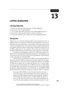
10-9 ADJUSTING THE COST OF CAPITAL FOR RISK As you will see in the chapters on capital budgeting that follow, the cost of capital is a key element in the capital budgeting process. Projects should be accepted if and only if their estimated returns exceed their costs of capital. Thus, the cost of capital is a “hurdle rate”—a project’s expected rate of return must “jump the hurdle” for it to be accepted. Moreover, investors require higher returns on riskier investments. Consequently, companies that are raising capital to take on risky projects will have higher costs of capital than companies that are investing in safer projects. Figure 10-1 illustrates the trade-off between risk and the cost of capital. Firm L is in a low-risk business and has a WACC of 8%. Firm A is an average-risk business with a WACC of 10%, while Firm H’s business is exposed to greater risk and consequently has a WACC of 12%. Thus, Firm L will accept a typical project if its expected return is above 8%. Firm A’s hurdle rate is 10%, while the corresponding hurdle rate for Firm H is 12%. It’s important to remember that the costs of capital for Firms L, A, and H in Figure 10-1 represent the overall, or composite, WACCs for the three firms and thus apply only to “typical” projects for each firm. However, different projects often have different risks, even for a given firm. Therefore, each project’s hurdle rate should reflect the risk of the project, not the risk associated with the firm’s average project as reflected in its composite WACC. Empirical studies do indicate that firms consider the risks of individual projects, but the studies also indicate that most firms regard most projects as having about the same risk as the firm’s average existing assets. Therefore, the WACC is used to evaluate most projects; but if a project has an especially high or low risk, the WACC will be adjusted up or down to account for the risk differential.

323

*ram* D:/Thomson_Learning_Projects/Brigham_Full_120614/z_production/z_3B2_3D_files/Brigham_0324597703_Ch.10.3d, 12/9/8, 13:52, page: 324

PROPERTY OF CENGAGE LEARNING

324

Part 4 Investing in Long-Term Assets: Capital Budgeting

Risk and the Cost of Capital

FIGURE 10-1 Rate of Return (%)

Acceptance Region WACC Firm H’s WACC

12.0 Rejection Region 10.0

0

Firm L’s WACC

Risk L

Risk A

Risk H

Risk

For example, assume that Firm A (the average-risk firm with a composite WACC of 10%) has two divisions, L and H. Division L has relatively little risk; and if it were operated as a separate firm, its WACC would be 7%. Division H has higher risk, and its divisional cost of capital is 13%. Since the two divisions are of equal size, Firm A’s composite WACC is calculated as 0.50(7%) þ 0.50(13%) ¼ 10%. However, it would be a mistake to use this 10% WACC for either division. To see this point, assume that Division L is considering a relatively low-risk project with an expected return of 9%, while Division H is considering a higher-risk project with an expected return of 11%. As shown in Figure 10-2, Division L’s project should be accepted because its return is above its risk-based cost of capital, whereas Division H’s project should be rejected. If the 10% corporate WACC was used by each division, the decision would be reversed: Division H would incorrectly accept its project, and Division L would incorrectly reject its project. In general, failing to adjust for differences in risk would lead the firm to accept too many risky projects and reject too many safe ones. Over time, the firm would become riskier, its WACC would increase, and its shareholder value would suffer. We will return to these issues in Chapter 12, when we consider different approaches for measuring project risk.

LF TEST

SE

8.0

Firm A’s WACC

Why is the cost of capital sometimes referred to as a “hurdle rate”? How should firms evaluate projects with different risks? Should all divisions within the same firm use the firm’s composite WACC for evaluating all capital budgeting projects? Explain.

*ram* D:/Thomson_Learning_Projects/Brigham_Full_120614/z_production/z_3B2_3D_files/Brigham_0324597703_Ch.10.3d, 12/9/8, 13:52, page: 325

PROPERTY OF CENGAGE LEARNING Chapter 10 The Cost of Capital

FIGURE 10-2

Divisional Cost of Capital

Rate of Return (%) WACC

Division H’s WACC 13.0

11.0

Project H

10.0 9.0

7.0

0

Composite WACC Project L

Division L’s WACC

Risk L

Risk A

Risk H

Risk

10-10 SOME OTHER PROBLEMS WITH COST OF CAPITAL ESTIMATES A number of issues related to the cost of capital have not been mentioned or were glossed over in this chapter. These topics are covered in advanced finance courses, but they deserve mention now to alert you to potential dangers and to provide a preview of some matters covered in advanced courses. 1. Depreciation-generated funds.21 The largest single source of capital for many firms is depreciation, yet we have not discussed how the cost of this capital is determined. In brief, depreciation cash flows can either be reinvested or returned to investors (stockholders and creditors). The cost of depreciationgenerated funds is thus an opportunity cost; and it is approximately equal to the WACC from retained earnings, preferred stock, and debt. Therefore, we can ignore it in our estimate of the WACC. 2. Privately owned firms. Our discussion of the cost of equity focused on publicly owned corporations, and we have concentrated on the rate of return required by public stockholders. However, there is a serious question about how to measure the cost of equity for a firm whose stock is not traded. Tax issues are also especially important in these cases. As a general rule, the same principles of cost of capital estimation apply to both privately held

21

See Table 3-3, the statement of cash flows, for an illustration of the cash flows provided from depreciation. Refer to advanced finance textbooks for a discussion on the treatment of depreciation-generated funds.

325

*ram* D:/Thomson_Learning_Projects/Brigham_Full_120614/z_production/z_3B2_3D_files/Brigham_0324597703_Ch.10.3d, 12/9/8, 13:52, page: 326

PROPERTY OF CENGAGE LEARNING

Part 4 Investing in Long-Term Assets: Capital Budgeting

3.

4.

5.

and publicly owned firms, but the problems of obtaining input data are somewhat different. Measurement problems. We cannot overemphasize the practical difficulties encountered when estimating the cost of equity. It is very difficult to obtain good input data for the CAPM, for g in the formula ^r s ¼ D1/P0 þ g, and for the risk premium in the formula rs ¼ Bond yield þ Risk premium. As a result, we can never be sure of the accuracy of our estimated cost of capital. Costs of capital for projects of differing risk. We touched briefly on the fact that different projects can differ in risk and, thus, in their required rates of return. However, it is difficult to measure a project’s risk (hence, to adjust the cost of capital for capital budgeting projects with different risks). Capital structure weights. In this chapter, we took as given the target capital structure and used it to calculate the WACC. As we shall see in the capital structure chapter, establishing the target capital structure is a major task in itself.

Although this list of problems appears formidable, the state of the art in cost of capital estimation is not in bad shape. The procedures outlined in this chapter can be used to obtain costs of capital estimates that are sufficiently accurate for practical purposes, so the problems listed previously merely indicate the desirability of refinements. The refinements are not unimportant, but the problems noted do not invalidate the usefulness of the procedures outlined in this chapter.

LF TEST

SE

326

Identify some problem areas in cost of capital analysis. Do these problems invalidate the cost of capital procedures discussed in this chapter? Explain.

TYING IT ALL TOGETHER We began this chapter by discussing the concept of the weighted average cost of capital. We then discussed the four capital components (debt, preferred stock, retained earnings, and new common equity) and the procedures used to estimate each component’s cost. Next, we calculated the WACC, which is a key element in capital budgeting. A key issue here is the weights that should be used to find the WACC. In general, companies consider a number of factors, then establish a target capital structure that is used to calculate the WACC. We discuss the target capital structure and its affect on the WACC in more detail in the capital structure chapter. The cost of capital is a key element in capital budgeting decisions, our focus in the following chapters. Indeed, capital budgeting as it should be done is impossible without a good estimate of the cost of capital; so you need to have a good understanding of cost of capital concepts before you move on.

*ram* D:/Thomson_Learning_Projects/Brigham_Full_120614/z_production/z_3B2_3D_files/Brigham_0324597703_Ch.10.3d, 12/9/8, 13:52, page: 327

PROPERTY OF CENGAGE LEARNING Chapter 10 The Cost of Capital

SELF-TEST QUESTIONS AND PROBLEMS (Solutions Appear in Appendix A) ST-1

ST-2

KEY TERMS Define the following terms: a.

Capital components

b.

Before-tax cost of debt, rd; after-tax cost of debt, rd(1 – T)

c.

Cost of preferred stock, rp

d.

Cost of retained earnings, rs; cost of new common stock, re

e.

Weighted average cost of capital, WACC

f.

Flotation cost, F; flotation cost adjustment; retained earnings breakpoint

WACC Lancaster Engineering Inc. (LEI) has the following capital structure, which it considers to be optimal: Debt Preferred stock Common equity

25% 15 60 100%

LEI’s expected net income this year is $34,285.72; its established dividend payout ratio is 30%; its federal-plus-state tax rate is 40%; and investors expect future earnings and dividends to grow at a constant rate of 9%. LEI paid a dividend of $3.60 per share last year, and its stock currently sells for $54.00 per share. LEI can obtain new capital in the following ways: l Preferred: New preferred stock with a dividend of $11.00 can be sold to the public at a price of $95.00 per share. l Debt: Debt can be sold at an interest rate of 12%. a.

Determine the cost of each capital component.

b.

Calculate the WACC.

c.

LEI has the following investment opportunities that are average-risk projects: Project

Cost at t = 0

A B C D E

$10,000 20,000 10,000 20,000 10,000

Rate of Return 17.4% 16.0 14.2 13.7 12.0

Which projects should LEI accept? Why?

QUESTIONS 10-1

How would each of the following scenarios affect a firm’s cost of debt, rd(1 – T); its cost of equity, rs; and its WACC? Indicate with a plus (þ), a minus (–), or a zero (0) if the factor would raise, would lower, or would have an indeterminate effect on the item in question. Assume for each answer that other things are held constant even though in some instances this would probably not be true. Be prepared to justify your answer but recognize that several of the parts have no single correct answer. These questions are designed to stimulate thought and discussion.

327

*ram* D:/Thomson_Learning_Projects/Brigham_Full_120614/z_production/z_3B2_3D_files/Brigham_0324597703_Ch.10.3d, 12/9/8, 13:52, page: 328

PROPERTY OF CENGAGE LEARNING

328

Part 4 Investing in Long-Term Assets: Capital Budgeting

EFFECT ON rd(1 − T)

rs

WACC

a. The corporate tax rate is lowered. b. The Federal Reserve tightens credit. c. The firm uses more debt; that is, it increases its debt/assets ratio. d. The dividend payout ratio is increased. e. The firm doubles the amount of capital it raises during the year. f. The firm expands into a risky new area. g. The firm merges with another firm whose earnings are countercyclical both to those of the first firm and to the stock market. h. The stock market falls drastically, and the firm’s stock price falls along with the rest of the stocks. i. Investors become more risk-averse. j. The firm is an electric utility with a large investment in nuclear plants. Several states are considering a ban on nuclear power generation.

10-2 10-3 10-4 10-5

Assume that the risk-free rate increases. What impact would this have on the cost of debt? What impact would it have on the cost of equity? How should the capital structure weights used to calculate the WACC be determined? Suppose a firm estimates its WACC to be 10%. Should the WACC be used to evaluate all of its potential projects, even if they vary in risk? If not, what might be “reasonable” costs of capital for average-, high-, and low-risk projects? The WACC is a weighted average of the costs of debt, preferred stock, and common equity. Would the WACC be different if the equity for the coming year came solely in the form of retained earnings versus some equity from the sale of new common stock? Would the calculated WACC depend in any way on the size of the capital budget? How might dividend policy affect the WACC?

PROBLEMS Easy Problems 1–5

10-1

10-2 10-3

10-4

AFTER-TAX COST OF DEBT The Heuser Company’s currently outstanding bonds have a 10% coupon and a 12% yield to maturity. Heuser believes it could issue new bonds at par that would provide a similar yield to maturity. If its marginal tax rate is 35%, what is Heuser’s after-tax cost of debt? COST OF PREFERRED STOCK Tunney Industries can issue perpetual preferred stock at a price of $47.50 a share. The stock would pay a constant annual dividend of $3.80 a share. What is the company’s cost of preferred stock, rp? COST OF COMMON EQUITY Percy Motors has a target capital structure of 40% debt and 60% common equity, with no preferred stock. The yield to maturity on the company’s outstanding bonds is 9%, and its tax rate is 40%. Percy’s CFO estimates that the company’s WACC is 9.96%. What is Percy’s cost of common equity? COST OF EQUITY WITH AND WITHOUT FLOTATION Javits & Sons’ common stock currently trades at $30.00 a share. It is expected to pay an annual dividend of $3.00 a share at the end of the year (D1 ¼ $3.00), and the constant growth rate is 5% a year. a.

What is the company’s cost of common equity if all of its equity comes from retained earnings?

*ram* D:/Thomson_Learning_Projects/Brigham_Full_120614/z_production/z_3B2_3D_files/Brigham_0324597703_Ch.10.3d, 12/9/8, 13:52, page: 329

PROPERTY OF CENGAGE LEARNING Chapter 10 The Cost of Capital

b.

10-5

Intermediate Problems 6–13

10-6

PROJECT SELECTION Midwest Water Works estimates that its WACC is 10.5%. The company is considering the following capital budgeting projects:

10-9

Size

A B C D E F G

$1 million 2 million 2 million 2 million 1 million 1 million 1 million

Rate of Return 12.0% 11.5 11.2 11.0 10.7 10.3 10.2

a.

Using the DCF approach, what is its cost of common equity?

b.

If the firm’s beta is 1.6, the risk-free rate is 9%, and the average return on the market is 13%, what will be the firm’s cost of common equity using the CAPM approach? If the firm’s bonds earn a return of 12%, based on the bond-yield-plus-risk-premium approach, what will be rs? Use the midpoint of the risk premium range discussed in Section 10-5 in your calculations. If you have equal confidence in the inputs used for the three approaches, what is your estimate of Carpetto’s cost of common equity?

d.

10-8

Project

Assume that each of these projects is just as risky as the firm’s existing assets and that the firm may accept all the projects or only some of them. Which set of projects should be accepted? Explain. COST OF COMMON EQUITY The future earnings, dividends, and common stock price of Carpetto Technologies Inc. are expected to grow 7% per year. Carpetto’s common stock currently sells for $23.00 per share; its last dividend was $2.00; and it will pay a $2.14 dividend at the end of the current year.

c.

10-7

If the company issued new stock, it would incur a 10% flotation cost. What would be the cost of equity from new stock?

COST OF COMMON EQUITY WITH AND WITHOUT FLOTATION The Evanec Company’s next expected dividend, D1, is $3.18; its growth rate is 6%; and its common stock now sells for $36.00. New stock (external equity) can be sold to net $32.40 per share. a.

What is Evanec’s cost of retained earnings, rs?

b.

What is Evanec’s percentage flotation cost, F?

c.

What is Evanec’s cost of new common stock, re?

COST OF COMMON EQUITY AND WACC Patton Paints Corporation has a target capital structure of 40% debt and 60% common equity, with no preferred stock. Its before-tax cost of debt is 12%, and its marginal tax rate is 40%. The current stock price is P0 ¼ $22.50. The last dividend was D0 ¼ $2.00, and it is expected to grow at a 7% constant rate. What is its cost of common equity and its WACC? WACC The Patrick Company’s cost of common equity is 16%, its before-tax cost of debt is 13%, and its marginal tax rate is 40%. The stock sells at book value. Using the following balance sheet, calculate Patrick’s WACC. Assets Cash Accounts receivable Inventories Plant and equipment, net Total assets

Liabilities and Equity $ 120 240 360 2,160 $2,880

Long-term debt Common equity Total liabilities and equity

$1,152 1,728 $2,880

329

*ram* D:/Thomson_Learning_Projects/Brigham_Full_120614/z_production/z_3B2_3D_files/Brigham_0324597703_Ch.10.3d, 12/9/8, 13:52, page: 330

PROPERTY OF CENGAGE LEARNING

330

Part 4 Investing in Long-Term Assets: Capital Budgeting

10-10

10-11

10-12

10-13

Challenging Problems 14–20

10-14

10-15

10-16

WACC Klose Outfitters Inc. believes that its optimal capital structure consists of 60% common equity and 40% debt, and its tax rate is 40%. Klose must raise additional capital to fund its upcoming expansion. The firm will have $2 million of new retained earnings with a cost of rs ¼ 12%. New common stock in an amount up to $6 million would have a cost of re ¼ 15%. Furthermore, Klose can raise up to $3 million of debt at an interest rate of rd ¼ 10% and an additional $4 million of debt at rd ¼ 12%. The CFO estimates that a proposed expansion would require an investment of $5.9 million. What is the WACC for the last dollar raised to complete the expansion? WACC AND PERCENTAGE OF DEBT FINANCING Hook Industries’ capital structure consists solely of debt and common equity. It can issue debt at rd ¼ 11%, and its common stock currently pays a $2.00 dividend per share (D0 ¼ $2.00). The stock’s price is currently $24.75, its dividend is expected to grow at a constant rate of 7% per year, its tax rate is 35%, and its WACC is 13.95%. What percentage of the company’s capital structure consists of debt? WACC Midwest Electric Company (MEC) uses only debt and common equity. It can borrow unlimited amounts at an interest rate of rd ¼ 10% as long as it finances at its target capital structure, which calls for 45% debt and 55% common equity. Its last dividend was $2, its expected constant growth rate is 4%, and its common stock sells for $20. MEC’s tax rate is 40%. Two projects are available: Project A has a rate of return of 13%, while Project B’s return is 10%. These two projects are equally risky and about as risky as the firm’s existing assets. a.

What is its cost of common equity?

b.

What is the WACC?

c.

Which projects should Midwest accept?

COST OF COMMON EQUITY WITH FLOTATION Ballack Co.’s common stock currently sells for $46.75 per share. The growth rate is a constant 12%, and the company has an expected dividend yield of 5%. The expected long-run dividend payout ratio is 25%, and the expected return on equity (ROE) is 16%. New stock can be sold to the public at the current price, but a flotation cost of 5% would be incurred. What would be the cost of new equity? COST OF PREFERRED STOCK INCLUDING FLOTATION Trivoli Industries plans to issue perpetual preferred stock with an $11.00 dividend. The stock is currently selling for $97.00; but flotation costs will be 5% of the market price, so the net price will be $92.15 per share. What is the cost of the preferred stock, including flotation? WACC AND COST OF COMMON EQUITY Kahn Inc. has a target capital structure of 60% common equity and 40% debt to fund its $10 billion in operating assets. Furthermore, Kahn Inc. has a WACC of 13%, a before-tax cost of debt of 10%, and a tax rate of 40%. The company’s retained earnings are adequate to provide the common equity portion of its capital budget. Its expected dividend next year (D1) is $3, and the current stock price is $35. a.

What is the company’s expected growth rate?

b.

If the firm’s net income is expected to be $1.1 billion, what portion of its net income is the firm expected to pay out as dividends? (Hint: Refer to Equation 9-4 in Chapter 9.)

COST OF COMMON EQUITY The Bouchard Company’s EPS was $6.50 in 2008, up from $4.42 in 2003. The company pays out 40% of its earnings as dividends, and its common stock sells for $36.00. a.

Calculate the past growth rate in earnings. (Hint: This is a 5-year growth period.)

b.

The last dividend was D0 ¼ 0.4($6.50) ¼ $2.60. Calculate the next expected dividend, D1, assuming that the past growth rate continues. What is Bouchard’s cost of retained earnings, rs?

c.

10-17

CALCULATION OF g AND EPS Sidman Products’ common stock currently sells for $60.00 a share. The firm is expected to earn $5.40 per share this year and to pay a year-end dividend of $3.60, and it finances only with common equity. a.

If investors require a 9% return, what is the expected growth rate?

b.

If Sidman reinvests retained earnings in projects whose average return is equal to the stock’s expected rate of return, what will be next years’ EPS? (Hint: Refer to Equation 9-4 in Chapter 9.)

*ram* D:/Thomson_Learning_Projects/Brigham_Full_120614/z_production/z_3B2_3D_files/Brigham_0324597703_Ch.10.3d, 12/9/8, 13:52, page: 331

PROPERTY OF CENGAGE LEARNING Chapter 10 The Cost of Capital

10-18

WACC AND OPTIMAL CAPITAL BUDGET Adams Corporation is considering four averagerisk projects with the following costs and rates of return: Project

Cost

1 2 3 4

$2,000 3,000 5,000 2,000

Expected Rate of Return 16.00% 15.00 13.75 12.50

The company estimates that it can issue debt at a rate of rd ¼ 10%, and its tax rate is 30%. It can issue preferred stock that pays a constant dividend of $5.00 per year at $49.00 per share. Also, its common stock currently sells for $36.00 per share; the next expected dividend, D1, is $3.50; and the dividend is expected to grow at a constant rate of 6% per year. The target capital structure consists of 75% common stock, 15% debt, and 10% preferred stock. a. What is the cost of each of the capital components?

10-19

b.

What is Adams’ WACC?

c.

Only projects with expected returns that exceed WACC will be accepted. Which projects should Adams accept?

ADJUSTING COST OF CAPITAL FOR RISK Ziege Systems is considering the following independent projects for the coming year:

Project

Required Investment

A B C D E F G H

$4 million 5 million 3 million 2 million 6 million 5 million 6 million 3 million

Rate of Return

Risk

14.0% 11.5 9.5 9.0 12.5 12.5 7.0 11.5

High High Low Average High Average Low Low

Ziege’s WACC is 10%, but it adjusts for risk by adding 2% to the WACC for high-risk projects and subtracting 2% for low-risk projects. a. Which projects should Ziege accept if it faces no capital constraints? b. c.

10-20

If Ziege can only invest a total of $13 million, which projects should it accept and what would be the dollar size of its capital budget? Suppose Ziege can raise additional funds beyond the $13 million, but each new increment (or partial increment) of $5 million of new capital will cause the WACC to increase by 1%. Assuming that Ziege uses the same method of risk adjustment, which projects should it now accept and what would be the dollar size of its capital budget?

WACC The following table gives Foust Company’s earnings per share for the last 10 years. The common stock, 7.8 million shares outstanding, is now (1/1/09) selling for $65.00 per share. The expected dividend at the end of the current year (12/31/09) is 55% of the 2008 EPS. Because investors expect past trends to continue, g may be based on the historical earnings growth rate. (Note that 9 years of growth are reflected in the 10 years of data.) Year

EPS

Year

EPS

1999

$3.90

2004

$5.73

2000

4.21

2005

6.19

2001

4.55

2006

6.68

2002

4.91

2007

7.22

2003

5.31

2008

7.80

331

*ram* D:/Thomson_Learning_Projects/Brigham_Full_120614/z_production/z_3B2_3D_files/Brigham_0324597703_Ch.10.3d, 12/9/8, 13:52, page: 332

PROPERTY OF CENGAGE LEARNING

332

Part 4 Investing in Long-Term Assets: Capital Budgeting

The current interest rate on new debt is 9%; Foust’s marginal tax rate is 40%; and its capital structure, considered to be optimal, is as follows: Debt Common equity Total liabilities and equity a. b.

$104,000,000 156,000,000 $260,000,000

Calculate Foust’s after-tax cost of debt and common equity. Calculate the cost of equity as rs ¼ D1/P0 þ g. Find Foust’s WACC.

COMPREHENSIVE/SPREADSHEET PROBLEM 10-21

CALCULATING THE WACC Here is the condensed 2008 balance sheet for Skye Computer Company (in thousands of dollars): 2008 Current assets Net fixed assets Total assets

$2,000 3,000 $5,000

Current liabilities Long-term debt Preferred stock Common stock Retained earnings Total common equity Total liabilities and equity

$ 900 1,200 250 1,300 1,350 $2,650 $5,000

Skye’s earnings per share last year were $3.20, the common stock sells for $55.00, last year’s dividend was $2.10, and a flotation cost of 10% would be required to sell new common stock. Security analysts are projecting that the common dividend will grow at a rate of 9% per year. Skye’s preferred stock pays a dividend of $3.30 per share, and new preferred could be sold at a price to net the company $30.00 per share. The firm can issue long-term debt at an interest rate (or before-tax cost) of 10%, and its marginal tax rate is 35%. The market risk premium is 5%, the risk-free rate is 6%, and Skye’s beta is 1.516. In its cost of capital calculations, the company considers only long-term capital; hence, it disregards current liabilities. a.

b. c.

d.

Calculate the cost of each capital component, that is, the after-tax cost of debt, the cost of preferred stock, the cost of equity from retained earnings, and the cost of newly issued common stock. Use the DCF method to find the cost of common equity. Now calculate the cost of common equity from retained earnings using the CAPM method. What is the cost of new common stock based on the CAPM? (Hint: Find the difference between re and rs as determined by the DCF method and add that differential to the CAPM value for rs.) If Skye continues to use the same capital structure, what is the firm’s WACC assuming that (1) it uses only retained earnings for equity? (2) If it expands so rapidly that it must issue new common stock?

*ram* D:/Thomson_Learning_Projects/Brigham_Full_120614/z_production/z_3B2_3D_files/Brigham_0324597703_Ch.10.3d, 12/9/8, 13:52, page: 333

PROPERTY OF CENGAGE LEARNING Chapter 10 The Cost of Capital

333

INTEGRATED CASE COLEMAN TECHNOLOGIES INC. 10-22

COST OF CAPITAL Coleman Technologies is considering a major expansion program that has been proposed by the company’s information technology group. Before proceeding with the expansion, the company must estimate its cost of capital. Assume that you are an assistant to Jerry Lehman, the financial vice president. Your first task is to estimate Coleman’s cost of capital. Lehman has provided you with the following data, which he believes may be relevant to your task. (1)

The firm’s tax rate is 40%.

(2)

The current price of Coleman’s 12% coupon, semiannual payment, noncallable bonds with 15 years remaining to maturity is $1,153.72. Coleman does not use short-term interest-bearing debt on a permanent basis. New bonds would be privately placed with no flotation cost.

(3)

The current price of the firm’s 10%, $100.00 par value, quarterly dividend, perpetual preferred stock is $111.10.

(4)

Coleman’s common stock is currently selling for $50.00 per share. Its last dividend (D0) was $4.19, and dividends are expected to grow at a constant rate of 5% in the foreseeable future. Coleman’s beta is 1.2, the yield on T-bonds is 7%, and the market risk premium is estimated to be 6%. For the bond-yield-plus-riskpremium approach, the firm uses a risk premium of 4%.

(5) Coleman’s target capital structure is 30% debt, 10% preferred stock, and 60% common equity. To structure the task somewhat, Lehman has asked you to answer the following questions. a.

(1)

What sources of capital should be included when you estimate Coleman’s WACC?

(2)

Should the component costs be figured on a before-tax or an after-tax basis?

(3)

Should the costs be historical (embedded) costs or new (marginal) costs?

b.

What is the market interest rate on Coleman’s debt and its component cost of debt?

c.

(1)

What is the firm’s cost of preferred stock?

(2)

Coleman’s preferred stock is riskier to investors than its debt, yet the preferred’s yield to investors is lower than the yield to maturity on the debt. Does this suggest that you have made a mistake? (Hint: Think about taxes.)

(1)

Why is there a cost associated with retained earnings?

(2)

What is Coleman’s estimated cost of common equity using the CAPM approach?

d. e.

What is the estimated cost of common equity using the DCF approach?

f.

What is the bond-yield-plus-risk-premium estimate for Coleman’s cost of common equity?

g.

What is your final estimate for rs?

h.

Explain in words why new common stock has a higher cost than retained earnings.

i.

(1)

What are two approaches that can be used to adjust for flotation costs?

(2)

Coleman estimates that if it issues new common stock, the flotation cost will be 15%. Coleman incorporates the flotation costs into the DCF approach. What is the estimated cost of newly issued common stock, considering the flotation cost?

j.

What is Coleman’s overall, or weighted average, cost of capital (WACC)? Ignore flotation costs.

k.

What factors influence Coleman’s composite WACC?

l.

Should the company use the composite WACC as the hurdle rate for each of its projects? Explain.

*ram* D:/Thomson_Learning_Projects/Brigham_Full_120614/z_production/z_3B2_3D_files/Brigham_0324597703_Ch.10.3d, 12/9/8, 13:52, page: 334

PROPERTY OF CENGAGE LEARNING

334

Part 4 Investing in Long-Term Assets: Capital Budgeting

Access the Thomson ONE problems through the CengageNOW™ web site. Use the Thomson ONE—Business School Edition online database to work this chapter’s questions.

Calculating 3M’s Cost of Capital In this chapter, we described how to estimate a company’s WACC, which is the weighted average of its costs of debt, preferred stock, and common equity. Most of the data we need to do this can be found in Thomson ONE. Here we walk through the steps used to calculate Minnesota Mining & Manufacturing’s (MMM) WACC.

Discussion Questions 1.

2.

3.

4.

As a first step, we need to estimate what percentage of MMM’s capital comes from long-term debt, preferred stock, and common equity. If we click on “FINANCIALS,” we can see from the balance sheet the amount of MMM’s long-term debt and common equity. (As of year-end 2007, MMM had no preferred stock.) Alternatively, under “Financial Ratios,” you can click on “WORLDSCOPE” and “ANNUAL BALANCE SHEET RATIOS.” Here you will find a recent measure of long-term debt as a percentage of total capital. Recall that the weights used in the WACC are based on the company’s target capital structure. If we assume that the company wants to maintain the same mix of capital that it currently has on its balance sheet, what weights should you use to estimate the WACC for MMM? (In the capital structure and leverage chapter, we might arrive at different estimates for these weights if we assume that MMM bases its target capital structure on the market values of debt and equity rather than on the book values.) Once again we can use the CAPM to estimate MMM’s cost of equity. Thomson ONE provides various estimates of beta—select the measure that you believe is best and combine this with your estimates of the risk-free rate and the market risk premium to obtain an estimate of its cost of equity. (See the Thomson ONE exercise in Chapter 8 for more details.) What is your estimate for MMM’s cost of equity? Why might it not make much sense to use the DCF approach to estimate MMM’s cost of equity? Next, we need to calculate MMM’s cost of debt. Unfortunately, Thomson ONE doesn’t provide a direct measure of the cost of debt. However, we can use different approaches to estimate it. One approach is to take the company’s long-term interest expense and divide it by the amount of long-term debt. This approach only works if the historical cost of debt equals the yield to maturity in today’s market (that is, if MMM’s outstanding bonds are trading at close to par). This approach may produce misleading estimates in years in which MMM issues a significant amount of new debt. For example, if a company issues a great deal of debt at the end of the year, the full amount of debt will appear on the year-end balance sheet, yet we still may not see a sharp increase in interest expense on the annual income statement because the debt was outstanding for only a small portion of the entire year. When this situation occurs, the estimated cost of debt will likely understate the true cost of debt. Another approach is to try to find this number in the notes to the company’s annual report by accessing the company’s home page and its Investor Relations section. Alternatively, you can go to other external sources, such as www.bondsonline.com, for corporate bond spreads, which can be used to find estimates of the cost of debt. Remember that you need the after-tax cost of debt to calculate a firm’s WACC, so you will need MMM’s tax rate (which has averaged about 32% in recent years). What is your estimate of MMM’s after-tax cost of debt? Putting all this information together, what is your estimate of MMM’s WACC? How confident are you in this estimate? Explain your answer.

*ram* D:/Thomson_Learning_Projects/Brigham_Full_120614/z_production/z_3B2_3D_files/Brigham_0324597703_Ch.11.3d, 12/9/8, 13:54, page: 335

ª STEPHEN STRATHDEE/SHUTTERSTOCK

PROPERTY OF CENGAGE LEARNING

11

CHAPTER

The Basics of Capital Budgeting

In early 2008, Boeing was involved in a titanic struggle with European consortium Airbus SAS for dominance of the commercial aircraft industry.1 Several years ago Airbus committed to spend $16 billion to develop the A380, the largest plane ever built. Boeing countered by announcing that it would spend $6 billion on a superefficient new plane, the 7E7 Dreamliner. Airbus then announced plans to spend another $6 billion on the A350, a competitor to the 7E7. Many detailed calculations went into these multibilliondollar investment decisions— development costs were estimated, the cost of each plane was forecasted, a sales price per plane was established, and the number of planes that would be sold through 2025 was predicted. Both companies projected negative cash flows for 5 or 6 years, then positive cash flows for

the following 20 years. Given their forecasted cash flows, both managements decided that taking on the projects would increase each company’s intrinsic value. Because the planes will compete with one another, either Boeing’s or Airbus’s forecast is probably incorrect. One will probably be a winner and the other a loser, and one set of stockholders will likely be happy and the other unhappy. As of the winter of 2008, both companies received orders for their planes, but both have encountered problems that have delayed the actual introduction of the aircraft. The winner is still undecided. Projects such as the A350, A380, and 7E7 receive a great deal of attention; but Boeing, Airbus, and other companies make a great many routine investment decisions every year, ranging from buying new trucks or machinery

1

Airbus SAS is owned by European Aeronautics Defense & Space Company (EADS), which is owned by the French government and several large European companies. Airbus was formed because the Europeans wanted to create an organization large enough to compete with Boeing.

335

Airbus, Boeing

Competition in the Aircraft Industry: Airbus vs. Boeing

*ram* D:/Thomson_Learning_Projects/Brigham_Full_120614/z_production/z_3B2_3D_files/Brigham_0324597703_Ch.11.3d, 12/9/8, 13:54, page: 336

PROPERTY OF CENGAGE LEARNING

336

Part 4 Investing in Long-Term Assets: Capital Budgeting

to purchasing computers and software to optimize inventory management. The techniques described in this

chapter are required to analyze projects of all types and sizes.

Sources: John Newhouse, Boeing Versus Airbus: The Inside Story of the Greatest International Competition in Business (New York: Random House, 2007).

PUTTING THINGS IN PERSPECTIVE Capital Budgeting The process of planning expenditures on assets with cash flows that are expected to extend beyond one year.

In the last chapter, we discussed the cost of capital. Now we turn to investment decisions involving fixed assets, or capital budgeting. Here capital refers to longterm assets used in production, while a budget is a plan that outlines projected expenditures during some future period. Thus, the capital budget is a summary of planned investments in long-term assets, and capital budgeting is the whole process of analyzing projects and deciding which ones to include in the capital budget. Boeing, Airbus, and other companies use the techniques in this chapter when deciding to accept or reject proposed capital expenditures. When you finish this chapter, you should be able to: Discuss capital budgeting. Calculate and use the major capital budgeting decision criteria, which are NPV, IRR, MIRR, and payback. Explain why NPV is the best criterion and how it overcomes problems inherent in the other methods. With an understanding of the theory of capital budgeting developed in this chapter, which uses simplified examples, you will be ready for the next chapter, where we discuss how cash flows are estimated, how risk is measured, and how capital budgeting decisions are made. l l

l

11-1 AN OVERVIEW OF CAPITAL BUDGETING The same concepts used in security valuation are also used in capital budgeting, but there are two major differences. First, stocks and bonds exist in the security markets, and investors select from the available set; firms, however, create capital budgeting projects. Second, for most securities, investors have no influence on the cash flows produced by their investments, whereas corporations have a major influence on projects’ results. Still, in both security valuation and capital budgeting, we forecast a set of cash flows, find the present value of those flows, and make the investment only if the PV of the inflows exceeds the investment’s cost. A firm’s growth, and even its ability to remain competitive and to survive, depends on a constant flow of ideas relating to new products, to improvements in existing products, and to ways of operating more efficiently. Accordingly, wellmanaged firms go to great lengths to develop good capital budgeting proposals. For example, the executive vice president of one successful corporation said that his company takes the following steps to generate projects: Our R&D department constantly searches for new products and ways to improve existing products. In addition, our Executive Committee, which consists of senior executives in marketing, production, and finance, identifies the

*ram* D:/Thomson_Learning_Projects/Brigham_Full_120614/z_production/z_3B2_3D_files/Brigham_0324597703_Ch.11.3d, 12/9/8, 13:54, page: 337

PROPERTY OF CENGAGE LEARNING Chapter 11 The Basics of Capital Budgeting

products and markets in which our company should compete, and the Committee sets long-run targets for each division. These targets, which are spelled out in the corporation’s strategic business plan, provide a general guide to the operating executives who must meet them. The operating executives then seek new products, set expansion plans for existing products, and look for ways to reduce production and distribution costs. Since bonuses and promotions are based on each unit’s ability to meet or exceed its targets, these economic incentives encourage our operating executives to seek out profitable investment opportunities. While our senior executives are judged and rewarded on the basis of how well their units perform, people further down the line are given bonuses and stock options for suggestions that lead to profitable investments. Additionally, a percentage of our corporate profit is set aside for distribution to nonexecutive employees, and we have an Employees’ Stock Ownership Plan (ESOP) to provide further incentives. Our objective is to encourage employees at all levels to keep an eye out for good ideas, especially those that lead to capital investments. Analyzing capital expenditure proposals is not costless—benefits can be gained, but analysis does have a cost. For certain types of projects, an extremely detailed analysis may be warranted, while for other projects, simpler procedures are adequate. Accordingly, firms generally categorize projects and then analyze them in each category somewhat differently: 1. Replacement: needed to continue current operations. One category consists of expenditures to replace worn-out or damaged equipment required in the production of profitable products. The only questions here are should the operation be continued and if so, should the firm continue to use the same production processes? If the answers are yes, the project will be approved without going through an elaborate decision process. 2. Replacement: cost reduction. This category includes expenditures to replace serviceable but obsolete equipment and thereby to lower costs. These decisions are discretionary, and a fairly detailed analysis is generally required. 3. Expansion of existing products or markets. These are expenditures to increase output of existing products or to expand retail outlets or distribution facilities in markets now being served. Expansion decisions are more complex because they require an explicit forecast of growth in demand, so a more detailed analysis is required. The go/no-go decision is generally made at a higher level within the firm. 4. Expansion into new products or markets. These investments relate to new products or geographic areas, and they involve strategic decisions that could change the fundamental nature of the business. Invariably, a detailed analysis is required, and the final decision is generally made at the top level of management. 5. Safety and/or environmental projects. Expenditures necessary to comply with government orders, labor agreements, or insurance policy terms fall into this category. How these projects are handled depends on their size, with small ones being treated much like the Category 1 projects. 6. Other projects. This catch-all includes items such as office buildings, parking lots, and executive aircraft. How they are handled varies among companies. 7. Mergers. In a merger, one firm buys another one. Buying a whole firm is different from buying an asset such as a machine or investing in a new airplane, but the same principles are involved. The concepts of capital budgeting underlie merger analysis. In general, relatively simple calculations, and only a few supporting documents, are required for replacement decisions, especially maintenance investments in

337

Strategic Business Plan A long-run plan that outlines in broad terms the firm’s basic strategy for the next 5 to 10 years.

*ram* D:/Thomson_Learning_Projects/Brigham_Full_120614/z_production/z_3B2_3D_files/Brigham_0324597703_Ch.11.3d, 12/9/8, 13:54, page: 338

PROPERTY OF CENGAGE LEARNING

338

Part 4 Investing in Long-Term Assets: Capital Budgeting

profitable plants. More detailed analyses are required for cost-reduction projects, for expansion of existing product lines, and especially for investments in new products or areas. Also, within each category, projects are grouped by their dollar costs: Larger investments require increasingly detailed analysis and approval at higher levels. Thus, a plant manager might be authorized to approve maintenance expenditures up to $10,000 using a relatively unsophisticated analysis, but the full board of directors might have to approve decisions that involve amounts greater than $1 million or expansions into new products or markets. If a firm has capable and imaginative executives and employees and if its incentive system is working properly, many ideas for capital investment will be advanced. Some ideas will be good ones, but others will not. Therefore, procedures must be established for screening projects. Companies use, and we discuss, the following criteria for deciding to accept or reject projects:2 1. Net Present Value (NPV) 2. Internal Rate of Return (IRR) 3. Modified Internal Rate of Return (MIRR) 4. Regular Payback 5. Discounted Payback The NPV is the best method, primarily because it addresses directly the central goal of financial management—maximizing shareholder wealth. However, all of the methods provide useful information, and all are used in practice at least to some extent.

How is capital budgeting similar to security valuation? How is it different?

SE

LF TEST

What are some ways that firms generate ideas for capital projects? Identify the major project classification categories and explain how and why they are used. What is the single best capital budgeting decision criterion?

11-2 NET PRESENT VALUE (NPV) Net Present Value (NPV) A method of ranking investment proposals using the NPV, which is equal to the present value of future net cash flows, discounted at the cost of capital.

The net present value (NPV) tells us how much a project contributes to shareholder wealth—the larger the NPV, the more value the project adds; and added value means a higher stock price.3 Thus, NPV is the best selection criterion. We use the data for Projects S and L shown in Table 11-1 to illustrate the calculation. The S stands for Short; the L, for Long. Project S is a short-term project in the sense that its cash inflows come in relatively soon, while L has more total cash inflows but they come in later in its life. The projects are equally risky, and they both have a 10% cost of capital. Furthermore, the cash flows have been adjusted to reflect

2 Two other rarely used criteria, the Profitability Index and the Accounting Rate of Return, are covered in Chapter 12 and its Web Extension of Eugene F. Brigham and Phillip R. Daves, Intermediate Financial Management, 9th ed. (Mason, OH: Thomson/South-Western, 2007). 3 We could divide the NPV by the number of shares outstanding to estimate a project’s effect on the stock price. However, given the lag between project acceptance and visible effects on earnings, this is rarely done for routine projects. However, for major projects, this procedure is useful.

*ram* D:/Thomson_Learning_Projects/Brigham_Full_120614/z_production/z_3B2_3D_files/Brigham_0324597703_Ch.11.3d, 12/9/8, 13:54, page: 339

PROPERTY OF CENGAGE LEARNING 339

Chapter 11 The Basics of Capital Budgeting

Table 11-1 A

Data on Projects S and L B

C

1 2 3 WACC for both projects: 4 Initial Cost: 5 0 6 Years: -$1,000 7 Project S: -$1,000 8 Project L:

D

E

F

10% After-Tax, End of Year Net Cash Inflows, CFt: 1 2 3 4 $500 $400 $300 $100 $100 $300 $400 $675

depreciation, taxes, and salvage values.4 The investment outlays shown as CF0 include fixed assets and any necessary investments in working capital, and cash flows come in at the end of the year. Finally, we show the table with an “Excel look,” which simply means adding row and column headings to a “regular” table. All of the calculations can be done easily with a financial calculator; but since some students may want to work with Excel, we show how problems would be set up in Excel. Do keep in mind, though, that Excel is not necessary. We find the NPVs as follows: 1. The present value of each cash flow is calculated, discounted at the project’s risk-adjusted cost of capital, r ¼ 10% in our example. 2. The sum of the discounted cash flows is defined as the project’s NPV. The equation for the NPV, set up with input data for Project S, is as follows: NPV ¼ CF0 þ ¼

CF1 CF2 CFN þ þ


þ ð1 þ rÞ1 ð1 þ rÞ2 ð1 þ rÞN

N X

CFt ð1 þ rÞt t¼0

NPVs ¼ $1,000 þ

G

11-1 $500 $400 $300 $100 þ þ þ ð1:10Þ1 ð1:10Þ4 ð1:10Þ2 ð1:10Þ3

Here CFt is the expected net cash flow at Time t, r is the project’s risk-adjusted cost of capital (or WACC), and N is its life. Projects generally require an initial investment—for example, developing the product, buying the equipment needed to make it, building a factory, and stocking inventory. The initial investment is a negative cash flow. For Projects S and L, only CF0 is negative; but for a large project such as Boeing’s 7E7, outflows occur for several years before cash inflows begin. Figure 11-1 shows the cash flow time line for Project S; the PV of each cash flow; and the sum of the PVs, which is by definition the NPV. The cost, at t ¼ 0, is –$1,000. The first positive cash flow is $500; and with a regular calculator, you could find its PV as $500/(1.10)1 ¼ $454.55. You could also find the PV of the $500 with a financial calculator. Other PVs could be found similarly, and the end result would be the numbers in the left column of the diagram. When we sum those numbers, the result is $78.82, which is NPVS. Note that the initial cost, the –$1,000, is not discounted because it occurs at Time 0. The NPV for Project L, $100.40, could be found similarly. 4 The most difficult aspect of capital budgeting is estimating the relevant cash flows. For simplicity, the net cash flows are treated as a given in this chapter, which allows us to focus on the rules for making capital budgeting decisions. However, in Chapter 12, we discuss cash flow estimation in detail. Also note that net working capital is defined as the increase in current assets required for a project minus the associated increases in payables and accruals. Thus, in capital budgeting, investment in working capital means the net amount that must be financed by investors.

Total Inflows $1,300 $1,475

*ram* D:/Thomson_Learning_Projects/Brigham_Full_120614/z_production/z_3B2_3D_files/Brigham_0324597703_Ch.11.3d, 12/9/8, 13:54, page: 340

PROPERTY OF CENGAGE LEARNING

340

Part 4 Investing in Long-Term Assets: Capital Budgeting

Finding the NPV for Projects S and L

FIGURE 11-1 A 11 12 Project S 13 14 15 16 17 18 NPVS = 19 20 NPVL =

B 0

r = 10%

-1,000.00 454.55 330.58 225.39 68.30 78.82 100.40

C 1

D 2

E 3

F 4

500

400

300

100

G

H

Sum = NPV for Project S NPVL found with the cash flow register of a calculator or Excel

The step-by-step procedure shown in Figure 11-1 is useful for illustrating how the NPV is calculated; but in practice (and on exams), it is far more efficient to use a financial calculator or Excel. Different calculators are set up somewhat differently; but as we discussed in Chapter 5, they all have a “cash flow register” that can be used to evaluate uneven cash flows such as those for Projects S and L. Equation 11-1 is programmed into these calculators, and all you must do is enter the cash flows (with the correct signs) along with r ¼ I/YR ¼ 10. Once the data have been entered and you press the NPV key, the answer, 78.82, appears on the screen.5 If you are familiar with Excel, you can use it to find the NPVs for S and L: NPVS ¼ $78:82 NPVL ¼ $100:40

Independent Projects Projects with cash flows that are not affected by the acceptance or nonacceptance of other projects. Mutually Exclusive Projects A set of projects where only one can be accepted.

The model used to obtain these values is provided in the chapter’s Excel model. If you want to know something about Excel, you should look at the model, as this is the way most people in practice find NPVs. Before using these NPVs in the decision process, we need to know whether Projects S and L are independent or mutually exclusive. Independent projects are projects whose cash flows are not affected by one another. If Wal-Mart was considering a new store in Boise and another in Atlanta, the projects would be independent; and if both had positive NPVs, Wal-Mart should accept both. Mutually exclusive projects, on the other hand, are projects where if one project is accepted, the other must be rejected. A conveyor belt system to move goods in a warehouse and a fleet of forklifts used for the same purpose would be mutually exclusive—accepting one implies rejecting the other. What should be the decision if Projects S and L are independent? In this case, both should be accepted because both have positive NPVs and thus add value to the firm. However, if they are mutually exclusive, Project L should be chosen because it has the higher NPV and thus adds more value than S. Here is a summary of the NPV decision rules: Independent projects: If NPV exceeds zero, accept the project. Mutually exclusive projects: Accept the project with the highest positive NPV. If no project has a positive NPV, reject them all.

5

The keystrokes for finding the NPV are shown for several calculators in the calculator tutorials provided on the text’s web site.

*ram* D:/Thomson_Learning_Projects/Brigham_Full_120614/z_production/z_3B2_3D_files/Brigham_0324597703_Ch.11.3d, 12/9/8, 13:54, page: 341

PROPERTY OF CENGAGE LEARNING Chapter 11 The Basics of Capital Budgeting

341

Since projects must be either independent or mutually exclusive, one or the other of these rules applies to every project.

Why is the NPV the primary capital budgeting decision criterion?

SE

LF TEST

What is the difference between independent and mutually exclusive projects? Projects SS and LL have the following cash flows: END-OF-YEAR CASH FLOWS

SS LL

0

1

2

$700 $700

$500 $100

WACC ¼ r ¼ 10%

3

$300 $300

$100 $600

If a 10% cost of capital is appropriate for both projects, what are their NPVs? (NPVSS ¼ $77.61; NPVLL ¼ $89.63) Which project(s) would you accept if SS and LL were (a) independent? (b) mutually exclusive?

11-3 INTERNAL RATE OF RETURN (IRR) In Chapter 7, we discussed the yield to maturity on a bond and we explained that if you hold it to maturity, you will earn the YTM on your investment. The YTM is found as the discount rate that forces the PV of the cash inflows to equal the price of the bond. This same concept is involved in capital budgeting when we calculate a project’s internal rate of return (IRR): A project’s IRR is the discount rate that forces the PV of the inflows to equal the cost. This is equivalent to forcing the NPV to equal zero. The IRR is an estimate of the project’s rate of return, and it is comparable to the YTM on a bond. To calculate the IRR, we begin with Equation 11-1 for the NPV, replace r in the denominator with the term IRR, and set the NPV equal to zero. This transforms Equation 11-1 into Equation 11-2, the one used to find the IRR. The rate that forces NPV to equal zero is the IRR.6 NPV ¼ CF0 þ 0 ¼

CF1 CF2 CFN þ þ


þ ¼ 0 ð1 þ IRRÞ1 ð1 þ IRRÞ2 ð1 þ IRRÞN

N X

CFt ð1 þ IRRÞt t¼0

NPVs ¼ 0 ¼ $1,000 þ

11-2 $500 ð1 þ IRRÞ1

þ

$400 ð1 þ IRRÞ2

þ

$300 ð1 þ IRRÞ3

þ

$100 ð1 þ IRRÞ4

Figure 11-2 illustrates the process of finding the IRR for Project S. Three procedures can be used: 1. Trial and Error. We could use a trial-and-error procedure—try a discount rate; see if the equation solves to zero; and if it doesn’t, try a different rate. We could

6

For a large, complex project like Boeing’s 7E7 jetliner, costs are incurred for several years before cash inflows begin. That means that we have a number of negative cash flows before the positive cash flows begin.

Internal Rate of Return (IRR) The discount rate that forces a project’s NPV to equal zero.

*ram* D:/Thomson_Learning_Projects/Brigham_Full_120614/z_production/z_3B2_3D_files/Brigham_0324597703_Ch.11.3d, 12/9/8, 13:54, page: 342

PROPERTY OF CENGAGE LEARNING

342

Part 4 Investing in Long-Term Assets: Capital Budgeting

Finding the IRR for Project S

FIGURE 11-2 A 24 25 Project S 26 27 28 29 30 31 32

B 0

IRR = 14.489%

-1,000.00 436.72 305.16 199.91 58.20 0.00

2.

C 1

D 2

E 3

F 4

500

400

300

100

G

H

= NPV at a discount rate of 14.489%. Since the NPV is zero, 14.489% must be the IRR.

then continue until we found the rate that forces the NPV to zero; that rate would be the IRR. For Project S, the IRR is 14.489%. Note, though, that the trialand-error procedure is so time-consuming that before computers and financial calculators were available, the IRR was rarely used. It’s useful to think about the trial-and-error procedure, but it’s far better to use a calculator or Excel to do the actual calculations. Calculator Solution. Enter the cash flows in the calculator’s cash flow register just as we did to find the NPV; then press the button labeled “IRR.” Instantly, you get the IRR. Here are the values for Projects S and L:7 IRRS ¼ 14:489% IRRL ¼ 13:549%

3.

Excel Solution. It is even easier to find IRRS using Excel, as we demonstrate in the chapter model.

Why is the discount rate that causes a project’s NPV to equal zero so special? The reason is that the IRR is an estimate of the project’s rate of return. If this return exceeds the cost of the funds used to finance the project, the difference will be a bonus that goes to the firm’s stockholders and causes the stock price to rise. Project S has an estimated return of 14.489% versus a 10% cost of capital, so its bonus is 4.489%. On the other hand, if the IRR is less than the cost of capital, stockholders must make up the shortfall, which will hurt the stock price. Note again that the IRR formula, Equation 11-2, is simply the NPV formula, Equation 11-1, solved for the particular discount rate that forces the NPV to zero. Thus, the same basic equation is used for both methods. The only difference is that with the NPV method, the discount rate is given and we find the NPV; with the IRR method, however, the NPV is set equal to zero and we find the interest rate that produces this equality. As we noted earlier, projects should be accepted or rejected depending on whether their NPVs are positive. However, the IRR is sometimes used (improperly

7

See the calculator tutorials on the text’s web site. Note that once the cash flows have been entered in the cash flow register, you can find the NPV and the IRR. To find the NPV, enter the interest rate (I/YR) and then press the NPV key. Then with no further entries, press the IRR key to find the IRR. Thus, once you set up the calculator to find the NPV, it is trivially easy to find the IRR. This is one reason most firms calculate the NPV and the IRR. If you calculate one, it is easy to calculate the other; and both provide information that decision makers find useful. The same is true with Excel.

*ram* D:/Thomson_Learning_Projects/Brigham_Full_120614/z_production/z_3B2_3D_files/Brigham_0324597703_Ch.11.3d, 12/9/8, 13:54, page: 343

PROPERTY OF CENGAGE LEARNING Chapter 11 The Basics of Capital Budgeting

WHY NPV IS BETTER THAN IRR Buffett University recently hosted a seminar on business methods for managers. A finance professor covered capital budgeting, explaining how to calculate the NPV and stating that it should be used to screen potential projects. In the Q&A session, Ed Wilson, the treasurer of an electronics firm, said that his firm used the IRR primarily because the CFO and the directors understood the selection of projects based on their rates of return but didn’t understand the NPV. Ed had tried to explain why the NPV was better, but he simply confused everyone; so the company stuck with the IRR. Now a meeting on the firm’s capital budget is coming up, and Ed asked the professor for a simple, easy-tounderstand explanation of why the NPV was better. The professor recommended the following extreme example. A firm with adequate access to capital and a 10% WACC is choosing between two equally risky, mutually exclusive projects. Project Large calls for investing $100,000 and then receiving $50,000 per year for 10 years, while Project Small calls for investing $1 and receiving $0.60 per year for 10 years. Here is each project’s NPV and IRR: Project Large ðLÞ

The IRR says choose S, but the NPV says take L. Intuitively, it’s obvious that the firm would be better off choosing the large project in spite of its lower IRR. With a cost of capital of only 10%, a 49% rate of return on a $100,000 investment is more profitable than a 59% return on a $1 investment. When Ed gave this example in his firm’s executive meeting on the capital budget, the CFO argued that this example was extreme and unrealistic and that no one would choose S in spite of its higher IRR. Ed agreed, but he asked the CFO where the line should be drawn between realistic and unrealistic examples. When Ed received no answer, he went on to say that (1) it’s hard to draw this line and (2) the NPV is always better because it tells us how much value each project will add, which is what the firm should maximize. The president was listening, and he declared Ed the winner. The company switched from IRR to NPV, and Ed is now the CFO.

Project Small ðSÞ

NPVL : $207,228:36

NPVS : $2:69

IRRL : 49:1%

IRRS : 59:4%

we believe) to rank projects and make capital budgeting decisions. When this is done, here are the decision rules: Independent projects: If IRR exceeds the project’s WACC, accept the project. If IRR is less than the project’s WACC, reject it. Mutually exclusive projects. Accept the project with the highest IRR, provided that IRR is greater than WACC. Reject all projects if the best IRR does not exceed WACC. The IRR is logically appealing—it is useful to know the rates of return on proposed investments. However, as we demonstrate in a later section, NPV and IRR can produce conflicting conclusions when a choice is being made between mutually exclusive projects; and when conflicts occur, the NPV is generally better.

In what sense is a project’s IRR similar to the YTM on a bond?

SE

LF TEST

The cash flows for projects SS and LL are as follows: END-OF-YEAR CASH FLOWS

SS LL

0

1

2

3

–$700 –$700

$500 $100

$300 $300

$100 $600

WACC ¼ r ¼ 10%

343

*ram* D:/Thomson_Learning_Projects/Brigham_Full_120614/z_production/z_3B2_3D_files/Brigham_0324597703_Ch.11.3d, 12/9/8, 13:54, page: 344

PROPERTY OF CENGAGE LEARNING

344

Part 4 Investing in Long-Term Assets: Capital Budgeting

What are the projects’ IRRs, and which one would the IRR method select if the firm had a 10% cost of capital and the projects were (a) independent or (b) mutually exclusive? (IRRSS ¼ 18.0%; IRRLL ¼ 15.6%)

11-4 MULTIPLE INTERNAL RATES OF RETURN8 A problem with the IRR is that under certain conditions, a project may have more than one IRR. First, note that a project is said to have normal cash flows if it has one or more cash outflows (costs) followed by a series of cash inflows. If, however, a cash outflow occurs sometime after the inflows have commenced, meaning that the signs of the cash flows change more than once, the project is said to have nonnormal cash flows. Examples: Normal: Nonnormal:

Multiple IRRs The situation where a project has two or more IRRs.

 

þ þ

þ þ

þ þ

þ þ

þ 

or  or 

 þ

 þ

þ þ

þ 

þ þ

þ þ

þ þ

An example of nonnormal flows would be a strip coal mine where the company spends money to buy the property and prepare the site for mining, has positive inflows for several years, and spends more money to return the land to its original condition. In such a case, the project might have two IRRs, that is, multiple IRRs.9 To illustrate multiple IRRs, suppose a firm is considering a potential strip mine (Project M) that has a cost of $1.6 million and will produce a cash flow of $10 million at the end of Year 1. Then at the end of Year 2, the firm must spend $10 million to restore the land to its original condition. Therefore, the project’s expected net cash flows are as follows (in millions): Year 0 Cash flows

End of Year 1

$1.6

þ$10

End of Year 2 –$10

We can substitute these values into Equation 11-2 and solve for the IRR: NPV ¼

$1:6 million ð1 þ IRRÞ

0

þ

$10 million $10 million ¼ 0 1 þ ð1 þ IRRÞ ð1 þ IRRÞ2

NPV equals 0 when IRR ¼ 25%, but it also equals 0 when IRR ¼ 400%.10 Therefore, Project M has an IRR of 25% and another of 400%, and we don’t know which one to use. This relationship is depicted graphically in Figure 11-3.11 The graph is constructed by plotting the project’s NPV at different discount rates. Note that no dilemma regarding Project M would arise if the NPV method was used; we would simply find the NPV and use it to evaluate the project.

8

This section is relatively technical, but it can be omitted without loss of continuity. Equation 11-2 is a polynomial of degree n; so it has n different roots, or solutions. All except one of the roots is an imaginary number when investments have normal cash flows (one or more cash outflows followed by cash inflows). So in the normal case, only one value of IRR appears. However, the possibility of multiple real roots (hence multiple IRRs) arises when negative net cash flows occur after the project has been placed in operation. 10 If you attempt to find Project M’s IRR with an HP calculator, you will get an error message, while TI calculators give only the IRR that’s closest to zero. When you encounter either situation, you can find the approximate IRRs by calculating NPVs using several different values for r ¼ I/YR, plotting NPV on the vertical axis with the corresponding discount rate on the horizontal axis of a graph, and seeing about where NPV ¼ 0. The intersection with the x-axis provides a rough idea of the IRRs’ values. With some calculators and with Excel, you can find both IRRs by entering guesses, as explained in the calculator and Excel tutorials. 11 Figure 11-3 is called an NPV profile. Profiles are discussed in more detail in Section 11-7. 9

*ram* D:/Thomson_Learning_Projects/Brigham_Full_120614/z_production/z_3B2_3D_files/Brigham_0324597703_Ch.11.3d, 12/9/8, 13:54, page: 345

PROPERTY OF CENGAGE LEARNING Chapter 11 The Basics of Capital Budgeting

Graph for Multiple IRRs: Project M

FIGURE 11-3 A 37 38 39 40 41 42 43 44 45 46 47 48 49 50 51 52 53 54 55 56 57 58 59 60 61 62 63 64 65 66

B

C

D

NPV (millions)

NPV = -$1.6 + $10/(1 + r) + -$10/(1 + r)2 $0.70

IRR = 400% IRR = 25%

0%

100%

200%

300%

400%

-$0.30

500%

Cost of Capital (%)

WACC = 10% Disc. Rate

NPV (millions)

10% 25% 110% 400% 500%

-$0.7736 $0.0000 $0.8943 $0.0000 -$0.2111

= IRR #1 = IRR #2

We would see that if Project M’s cost of capital was 10%, its NPV would be –$0.7736 million and the project should be rejected. However, if r was between 25% and 400%, NPV would be positive, but those numbers would not be realistic or useful for anything.

What condition regarding cash flows would cause more than one IRR to exist?

SE

LF TEST

E

Project MM has the following cash flows: END-OF-YEAR CASH FLOWS 0

1

2

3

–$1,000

$2,000

$2,000

–$3,350

Calculate MM’s NPV at discount rates of 0%, 10%, 12.2258%, 25%, 122.1470%, and 150%. What are MM’s IRRs? If the cost of capital is 10%, should the project be accepted or rejected? (NPVs range from –$350 to +$164 and then back down to –$94; the IRRs are 12.23% and 122.15%.)

345

*ram* D:/Thomson_Learning_Projects/Brigham_Full_120614/z_production/z_3B2_3D_files/Brigham_0324597703_Ch.11.3d, 12/9/8, 13:54, page: 346

PROPERTY OF CENGAGE LEARNING

346

Part 4 Investing in Long-Term Assets: Capital Budgeting

11-5 REINVESTMENT RATE ASSUMPTIONS12 The NPV calculation is based on the assumption that cash inflows can be reinvested at the project’s risk-adjusted WACC, whereas the IRR calculation is based on the assumption that cash flows can be reinvested at the IRR. To see why this is so, consider the following diagram, which was first used in Chapter 5 to illustrate the future value of $100 when the interest rate was 5%.

0

5%

Going from PV to FV: PV = $100.00

1

5%

$105.00

2

5%

$110.25

3 $115.76 = FV

Observe that the FV calculation assumes that the interest earned during each year can be reinvested to earn the same 5% in each succeeding year. Now recall that when we found the PV, we reversed the process, discounting rather than compounding at the 5% rate. This diagram was used to demonstrate this point:

0 Going from FV to PV: PV = $100.00

5%

1 $105.00

5%

2 $110.25

5%

3 $115.76 = FV

This led to the following conclusion: When we calculate a present value, we are implicitly assuming that cash flows can be reinvested at a specified interest rate, 5% in our example. This applies to Projects S and L: When we calculated their NPVs, we discounted at the WACC, 10%, which means that we were assuming that their cash flows could be reinvested at 10%. Now consider the IRR. In Section 11-3 we presented a cash flow diagram set up to show the PVs of the cash flows when discounted at the IRR. We saw that the sum of the PVs is equal to the cost at a discount rate of 14.489%; so by definition, 14.489% is the IRR. Now we can ask this question: What reinvestment rate is built into the IRR? Since discounting at a given rate assumes that cash flows can be reinvested at that same rate, the IRR assumes that cash flows are reinvested at the IRR. The NPV assumes reinvestment at the WACC, while the IRR assumes reinvestment at the IRR. Which assumption is more reasonable? For most firms, assuming reinvestment at the WACC is more reasonable for the following reasons: If a firm has reasonably good access to the capital markets, it can raise all the capital it needs at the going rate, which in our example is 10%. Since the firm can obtain capital at 10%, if it has investment opportunities with positive NPVs, it should take them on and it can finance them at a 10% cost. If the firm uses internally generated cash flows from past projects rather than external capital, this will save it the 10% cost of capital. Thus, 10% is the opportunity cost of the cash flows, and that is the effective return on reinvested funds. l

l

l

To illustrate all this, suppose a project’s IRR is 50%, the firm’s WACC is 10%, and the firm has adequate access to the capital markets. Thus, the firm can raise all the capital it needs at the 10% rate. Unless the firm is a monopoly, the 50% return would attract competition, which would make it hard to find new projects with a similar high return, which is what the IRR assumes. Moreover, even if the firm 12

This section gives a theoretical explanation of the key difference between NPV and IRR. However, it is relatively technical; so if time is a constraint, professors may decide to have students skip it and just read the box titled, “Why NPV Is Better Than IRR,” which appears earlier in the chapter.

*ram* D:/Thomson_Learning_Projects/Brigham_Full_120614/z_production/z_3B2_3D_files/Brigham_0324597703_Ch.11.3d, 12/9/8, 13:54, page: 347

PROPERTY OF CENGAGE LEARNING Chapter 11 The Basics of Capital Budgeting

347

does find such projects, it could take them on with external capital that costs 10%. The logical conclusion is that the original project’s cash flows will save the 10% cost of the external capital, and that is the effective return on those flows. If a firm does not have good access to external capital and if it has many potential projects with high IRRs, it might be reasonable to assume that a project’s cash flows could be reinvested at rates close to their IRRs. However, that situation rarely exists: Firms with good investment opportunities generally do have good access to debt and equity markets. Our conclusion is that the assumption built into the IRR—that cash flows can be reinvested at the IRR—is flawed, whereas the assumption built into the NPV— that cash flows can be reinvested at the WACC—is generally correct. Moreover, if the true reinvestment rate is less than the IRR, the true rate of return on the investment must be less than the calculated IRR; thus, the IRR is misleading as a measure of projects’ profitability. This point is discussed further in the next section.

SE

LF TEST

Why is it true that a reinvestment rate is implicitly assumed whenever we find the present value of a future cash flow? Would it be possible to find the PV of a FV without specifying an implicit reinvestment rate? (PVs are the reverse of FVs. We need r to find FV; hence, we need r to find the PV.) What reinvestment rate is built into the NPV calculation? the IRR calculation? (WACC, IRR) For a firm that has adequate access to capital markets, is it more reasonable to assume reinvestment at the WACC or the IRR? (WACC)

11-6 MODIFIED INTERNAL RATE OF RETURN (MIRR)13 It is logical for managers to want to know the expected rate of return on investments, and this is what the IRR is supposed to tell them. However, the IRR is based on the assumption that projects’ cash flows can be reinvested at the IRR. This assumption is generally incorrect, and this causes the IRR to overstate the project’s true return.14 Given this fundamental flaw, is there a percentage evaluator that is better than the regular IRR? The answer is yes—we can modify the IRR to make it a better measure of profitability. This new measure, the Modified IRR (MIRR), is illustrated for Project S in Figure 11-4. It is similar to the regular IRR except that it is based on the assumption that cash flows are reinvested at the WACC (or some other explicit rate if that is a more reasonable assumption). Refer to Figure 11-4 as you read about its construction. 1. Project S has just one outflow, the minus $1,000 at t ¼ 0. Since it occurs at Time 0, it is not discounted and its PV is –$1,000. If the project had additional outflows, we would find the PV at t ¼ 0 for each one and sum them for use in the MIRR calculation. 2. Next, we find the future value of each inflow compounded at the WACC out to the “terminal year,” which is the year the last inflow is received. We assume that cash flows are reinvested at the WACC. For Project S, the first cash flow,

13

Again, this section is relatively technical, but it too can be omitted without loss of continuity. The IRR overstates the expected return for accepted projects because cash flows cannot generally be reinvested at the IRR. Therefore, the average IRR for accepted projects is greater than the true expected rate of return. This imparts an upward bias on corporate projections based on IRRs.

14

Modified IRR (MIRR) The discount rate at which the present value of a project’s cost is equal to the present value of its terminal value, where the terminal value is found as the sum of the future values of the cash inflows, compounded at the firm’s cost of capital.

*ram* D:/Thomson_Learning_Projects/Brigham_Full_120614/z_production/z_3B2_3D_files/Brigham_0324597703_Ch.11.3d, 12/9/8, 13:54, page: 348

PROPERTY OF CENGAGE LEARNING

348

Part 4 Investing in Long-Term Assets: Capital Budgeting

Finding the MIRR for Projects S and L, WACC ¼ 10%

FIGURE 11-4 A

B

C

D

1

2

E WACC = 3

69

0

r = 10%

F 10% 4

70 Project S
$1,000.00 $500 $400 $300 $100.00 71 $330.00 72 $484.00 73 $665.50 74 Terminal Value (TV) =
$1,000.00 $1,579.50 75 76 $1,000 = TV/(1MIRR)N = $1,579.50/(1MIRR)4. Solve for MIRR with calculator or Excel. 77 Calculator: N = 4, PV =
1000, PMT = 0, FV = 1579.5. Press I/YR to get: 78 Rate = MIRR Excel: = RATE(F70,0,B71,F75) 79 Direct Excel calculation, MIRR function: =MIRR(B71:F71,F69,F69)

3.

4.

G

H

12.11% 12.11% 12.11%

$500, is compounded at WACC ¼ 10% for 3 years and it grows to $665.50. The second inflow, $400, grows to $484.00; the third, to $330.00. The last inflow is received at the end, so it is not compounded at all. The sum of the future values, $1,579.50, is called the “terminal value,” or TV. We now have the cost at t ¼ 0, –$1,000, and the TV at Year 4, $1,579.50. There is some discount rate that will cause the PV of the terminal value to equal the cost. That interest rate is defined as the MIRR. In a calculator, enter N ¼ 4, PV ¼ –1000, PMT ¼ 0, and FV ¼ 1579.50. Then when you press the I/YR key, you get the MIRR, 12.11%. The MIRR can be found in a number of ways. Figure 11-4 illustrates how the MIRR is calculated: We compound each cash inflow, sum them to determine the TV, and then find the rate that causes the PV of the TV to equal the cost. That rate is 12.11%. However, some of the better calculators have a built-in MIRR function that streamlines the process, as does Excel. We explain how to use the calculator function in the calculator tutorials, and we explain how to find MIRR with Excel in the chapter Excel model.15

The MIRR has two significant advantages over the regular IRR. First, whereas the regular IRR assumes that the cash flows from each project are reinvested at the 15

Equation 11-2a summarizes these steps.

N X COFt t ¼ t ¼ 0 ð1 þ rÞ

11-2a

PV costs ¼

N X CIFt ð1 þ rÞNt t¼0

ð1 þ MIRRÞN TV ð1 þ MIRRÞN

COFt is the cash outflow at time t, and CIFt is the cash inflow at time t. The left term is the PV of the investment outlays when discounted at the cost of capital; the numerator of the second term is the compounded value of the inflows, assuming the inflows are reinvested at the cost of capital. The MIRR is the discount rate that forces the PV of the TV to equal the PV of the costs. Also note that there are alternative definitions for the MIRR. One difference relates to whether negative cash flows, after the positive cash flows begin, should be compounded and treated as part of the TV or discounted and treated as a cost. A related issue is whether negative and positive flows in a given year should be netted or treated separately. For a complete discussion, see William R. McDaniel, Daniel E. McCarty, and Kenneth A. Jessell, “Discounted Cash Flow with Explicit Reinvestment Rates: Tutorial and Extension,” The Financial Review, August 1988, pp. 369–385 and David M. Shull, “Interpreting Rates of Return: A Modified Rate of Return Approach,” Financial Practice and Education, Fall 1993, pp. 67–71.

*ram* D:/Thomson_Learning_Projects/Brigham_Full_120614/z_production/z_3B2_3D_files/Brigham_0324597703_Ch.11.3d, 12/9/8, 13:54, page: 349

PROPERTY OF CENGAGE LEARNING Chapter 11 The Basics of Capital Budgeting

349

IRR, the MIRR assumes that cash flows are reinvested at the cost of capital (or some other explicit rate). Since reinvestment at the IRR is generally not correct, the MIRR is generally a better indicator of a project’s true profitability. Second, the MIRR eliminates the multiple IRR problem—there can never be more than one MIRR, and it can be compared with the cost of capital when deciding to accept or reject projects. Our conclusion is that the MIRR is better than the regular IRR; however, this question remains: Is MIRR as good as the NPV? Here are our conclusions: For independent projects, the NPV, IRR, and MIRR always reach the same accept/reject conclusion; so the three criteria are equally good when evaluating independent projects. However, if projects are mutually exclusive and they differ in size, conflicts can arise. In such cases, the NPV is best because it selects the project that maximizes value.16 Our overall conclusions are that (1) the MIRR is superior to the regular IRR as an indicator of a project’s “true” rate of return but that (2) NPV is better than IRR and MIRR when choosing among competing projects. l

l

l

SE

LF TEST

What’s the primary difference between the MIRR and the regular IRR? (reinvestment rate) Which provides a better estimate of a project’s “true” rate of return, the MIRR or the regular IRR? Explain. Projects A and B have the following cash flows:

A B

0

1

2

$1,000 $1,000

$1,150 $ 100

$ 100 $1,300

Their cost of capital is 10%. What are the projects’ IRRs, MIRRs, and NPVs? Which project would each method select? (IRRA ¼ 23.1%, IRRB ¼ 19.1%; MIRRA ¼ 16.8%, MIRRB ¼18.7%; NPVA ¼ $128.10, NPVB ¼ $165.29)

11-7 NPV PROFILES Figure 11-5 presents the net present value profile for Project S. To make the profile, we find the project’s NPV at a number of different discount rates and then plot those values to create a graph. Note that at a zero cost of capital, the NPV is simply the net total of the undiscounted cash flows, $1,300 – $1,000 ¼ $300. This value is plotted as the vertical axis intercept. Also recall that the IRR is the discount rate that causes the NPV to equal zero, so the discount rate at which the profile line crosses the horizontal axis is the project’s IRR. When we connect the data points, we have the NPV profile.17

16

See Brigham and Daves, Intermediate Financial Management, 9th ed. (Mason, OH: South-Western, 2007), pp. 412–413. 17 Notice that the NPV profile is curved—it is not a straight line. NPV approaches CF0 , which is the –$1,000 project cost, as the discount rate increases toward infinity. The reason is that at an infinitely high cost of capital, all the PVs of the inflows would be zero; so NPV at r ¼ ∞ must be CF0. We should also note that under certain conditions, the NPV profiles can cross the horizontal axis several times or never cross it. This point was discussed in Section 11-4.

Net Present Value Profile A graph showing the relationship between a project’s NPV and the firm’s cost of capital.

*ram* D:/Thomson_Learning_Projects/Brigham_Full_120614/z_production/z_3B2_3D_files/Brigham_0324597703_Ch.11.3d, 12/9/8, 13:54, page: 350

PROPERTY OF CENGAGE LEARNING

350

Part 4 Investing in Long-Term Assets: Capital Budgeting

NPV Profile for Project S

FIGURE 11-5 NPV ($) 300

NPV = 0, so IRRs = 14.489% IRR > r = 10%, so accept

At r = 10%, NPV > 0, so accept

200

100

0

5

15

10

20

–100 Cost of Capital (%)

Cost of Capital

NPVs

0% 5 10 14.489 15 20

IRRs ¼

$300.00 180.00 78.82 0.00 8.33 83.72

Now consider Figure 11-6, which shows two NPV profiles—one for Project S and one for L—and note the following points: The IRRs are fixed, and S has the higher IRR regardless of the cost of capital. However, the NPVs vary depending on the actual cost of capital. The two NPV profile lines cross at a cost of capital of 11.975%, which is called the crossover rate. The crossover rate can be found by calculating the IRR of the differences in the projects’ cash flows, as demonstrated: l l l

Crossover Rate The cost of capital at which the NPV profiles of two projects cross and, thus, at which the projects’ NPVs are equal.

Project S Project L ΔCFs – CFL IRR Δ ¼ l

0

1

2

3

4

–$1,000 –$1,000

$500 $100

$400 $300

$300 $400

$100 $675

$400

$100

–$100

–$575

$

0

11.975% ¼ Crossover Rate

Project L has the higher NPV if the cost of capital is less than the crossover rate, but S has the higher NPV if the cost of capital is greater than that rate.

Notice that Project L has the steeper slope, indicating that a given increase in the cost of capital causes a larger decline in NPVL than in NPVS. To see why this is so, recall that L’s cash flows come in later than those of S. Therefore, L is a long-term project and S is a short-term project. Next, recall the equation for the NPV: NPV ¼ CF0 þ

CF1 CF2 CFN 1 þ 2 þ


þ ð1 þ rÞ ð1 þ rÞ ð1 þ rÞN

*ram* D:/Thomson_Learning_Projects/Brigham_Full_120614/z_production/z_3B2_3D_files/Brigham_0324597703_Ch.11.3d, 12/9/8, 13:54, page: 351

PROPERTY OF CENGAGE LEARNING Chapter 11 The Basics of Capital Budgeting

NPV Profiles for Projects S and L

FIGURE 11-6 NPV ($) 500

400

L At r = 10%, NPVL > NPVs, but IRRs > IRRL, so there is a conflict

300 S

Crossover rate; conflict if r is to the left, no conflict if r is to the right

200 IRRs

100 0

5

20

10 15 IRRL

–100

Cost of Capital (%)

Cost of Capital

Crossover ¼ IRRL ¼ IRRS ¼

0% 5 10 11.975 13.549 14.489 15 20

NPVs

NPVL

$300.00 180.42 78.82 42.84 15.64 0.00 8.33 83.72

$475.00 268.21 100.40 42.84 0.00 24.37 37.26 151.33

Now recognize that the impact of an increase in the cost of capital is much greater on distant than near-term cash flows, as we demonstrate here: Effect of doubling r on a Year 1 cash flow: $100 ¼ $95:24 ð1:05Þ1 $100 ¼ $90:91 PV of $100 due in 1 year @ r ¼ 10%: ð1:10Þ1 $95:24  $90:91 Percentage decline due to higher r ¼ ¼ 4:5% $95:24 PV of $100 due in 1 year @ r ¼ 5%:

Effect of doubling r on a Year 20 cash flow: PV of $100 due in 20 years @ r ¼ 5%:

$100

¼ $37:69 ð1:05Þ20 $100 PV of $100 due in 20 years @ r ¼ 10%: ¼ $14:86 ð1:10Þ20 $37:69  $14:86 ¼ 60:6% Percentage decline due to higher r ¼ $37:69

351

*ram* D:/Thomson_Learning_Projects/Brigham_Full_120614/z_production/z_3B2_3D_files/Brigham_0324597703_Ch.11.3d, 12/9/8, 13:54, page: 352

PROPERTY OF CENGAGE LEARNING

352

Part 4 Investing in Long-Term Assets: Capital Budgeting

Thus, a doubling of the discount rate results in only a 4.5% decline in the PV of a Year 1 cash flow, but the same discount rate increase causes the PV of a Year 20 cash flow to fall by more than 60%. Therefore, if a project has most of its cash flows coming in the later years, its NPV will decline sharply if the cost of capital increases; but a project whose cash flows come earlier will not be severely penalized by high capital costs. Most of Project L’s cash flows come in its later years; so if the cost of capital is high, L is hurt much worse than Project S. Therefore, Project L’s NPV profile has the steeper slope. Sometimes the NPV and IRR methods produce conflicting results. We can use NPV profiles to see when conflicts can and cannot arise. Independent Projects. If an independent project with normal cash flows is being evaluated, the NPV and IRR criteria always lead to the same accept/reject decision: If NPV says accept, IRR also says accept, and vice versa. To see why this is so, look at Figure 11-5 and notice that (1) the IRR says accept if the project’s cost of capital is less than (or to the left of) the IRR and (2) if the cost of capital is less than the IRR, the NPV will be positive. Thus, at any cost of capital less than 14.489%, Project S will be recommended by both the NPV and IRR criteria; but both methods reject the project if the cost of capital is greater than 14.489%. A similar graph could be used for Project L or any other normal project, and we would always reach the same conclusion: For normal, independent projects, if the IRR says accept, so will the NPV. Mutually Exclusive Projects. Assume that Projects S and L are mutually exclusive rather than independent. Therefore, we can choose either S or L, or we can reject both; but we can’t accept both. Now look at Figure 11-6 and note these points: As long as the cost of capital is greater than the crossover rate, 11.975%, both methods agree that Project S is better: NPVS > NPVL and IRRS > IRRL. Therefore, if r is greater than the crossover rate, no conflict occurs. However, if the cost of capital is less than the crossover rate, a conflict arises: NPV ranks L higher, but IRR ranks S higher. l

l

Two basic conditions cause NPV profiles to cross and thus lead to conflicts:18 1. Timing differences. If most of the cash flows from one project come in early while most of those from the other project come in later, as occurred with Projects S and L, the NPV profiles may cross and result in a conflict. 2. Project size (or scale) differences. If the amount invested in one project is larger than the other, this too can lead to profiles crossing and a resulting conflict. When size or timing differences occur, the firm will have different amounts of funds to invest in the various years depending on which of the two mutually exclusive projects it chooses. If it chooses S, it will have more funds to invest in Year 1 because S has a higher inflow that year. Similarly, if one project costs more than the other, the firm will have more money to invest at t ¼ 0 if it selects the smaller project. Given this situation, the rate of return at which differential cash flows can be reinvested is a critical issue. We saw earlier that the NPV assumes reinvestment at the cost of capital and that this is generally the best assumption. Therefore, when conflicts exist between mutually exclusive projects, use the NPV method.

18

Of course, mutually exclusive projects can differ with respect to both scale and timing. Also, if mutually exclusive projects have different lives (as opposed to different cash flow patterns over a common life), this introduces further complications; and for meaningful comparisons, some mutually exclusive projects must be evaluated over a common life. This point is discussed later in the text and in an appendix on the text’s web site.

*ram* D:/Thomson_Learning_Projects/Brigham_Full_120614/z_production/z_3B2_3D_files/Brigham_0324597703_Ch.11.3d, 12/9/8, 13:54, page: 353

PROPERTY OF CENGAGE LEARNING Chapter 11 The Basics of Capital Budgeting

SE

LF TEST

353

Describe in words how an NPV profile is constructed. How are the intercepts of the x- and y-axes determined? What is the crossover rate, and how does its value relative to the cost of capital determine whether a conflict exists between NPV and IRR? What two characteristics can lead to conflicts between the NPV and the IRR when evaluating mutually exclusive projects?

11-8 PAYBACK PERIOD NPV is the most commonly used method today; but historically, the first selection criterion was the payback period, defined as the number of years required to recover the funds invested in a project from its operating cash flows. Equation 11-3 is used for the calculation, and the process is diagrammed in Figure 11-7. We start with the project’s cost, a negative, and then add the cash inflow for each year until the cumulative cash flow turns positive. The payback year is the year prior to full recovery plus a fraction equal to the shortfall at the end of that year divided by the cash flow during the full recovery year:19 11-3

Unrecovered cost Number of at start of year Payback ¼ years prior to þ Cash flow during full recovery full recovery year

The shorter the payback, the better the project. Therefore, if the firm requires a payback of three years or less, S would be accepted, but L would be rejected. If the projects were mutually exclusive, S would be ranked over L because of its shorter payback.

FIGURE 11-7 Project S

Years

0

Cash flow Cumulative cash flow


1,000
1,000

Payback S = 2 + 100/300 =

2.33

Project L

19

Payback Calculations

Years

0

Cash flow Cumulative cash flow


1,000
1,000

Payback L = 3 + 200/675 =

3.30

1 500
500

1 100
900

2 400
100

3

4

300 200

100 300

3

4

2 300
600

400
200

Equation 11-3 assumes that cash flows come in uniformly during the full recovery year.

675 475

Payback Period The length of time required for an investment’s net revenues to cover its cost.

*ram* D:/Thomson_Learning_Projects/Brigham_Full_120614/z_production/z_3B2_3D_files/Brigham_0324597703_Ch.11.3d, 12/9/8, 13:54, page: 354

PROPERTY OF CENGAGE LEARNING

354

Part 4 Investing in Long-Term Assets: Capital Budgeting

Discounted Payback The length of time required for an investment’s cash flows, discounted at the investment’s cost of capital, to cover its cost.

FIGURE 11-8 Project S

The payback has three flaws: (1) All dollars received in different years are given the same weight (i.e., the time value of money is ignored). (2) Cash flows beyond the payback year are given no consideration regardless of how large they might be. (3) Unlike the NPV, which tells us how much wealth a project adds, and the IRR, which tells us how much a project yields over the cost of capital, the payback merely tells us when we recover our investment. There is no necessary relationship between a given payback and investor wealth maximization, so we do not know what an acceptable payback is. The firm might use 2 years, 3 years, or any other number as the minimum acceptable payback; but the choice is purely arbitrary. To counter the first criticism, analysts developed the discounted payback. Here cash flows are discounted at the WACC; then those discounted cash flows are used to find the payback. In Figure 11-8, we calculate the discounted paybacks for S and L assuming that both have a 10% cost of capital. Each inflow is divided by (1 þ r)t ¼ (1.10)t, where t is the year in which the cash flow occurs and r is the project’s cost of capital; and those PVs are used to find the payback. Project S’s discounted payback is 2.95, while L’s is 3.78. Note that the payback is a “break-even” calculation in the sense that if cash flows come in at the expected rate, the project will break even. However, since the regular payback doesn’t consider the cost of capital, it doesn’t specify the true break-even year. The discounted payback does consider capital costs; but it still disregards cash flows beyond the payback year, which is a serious flaw. Further, if mutually exclusive projects vary in size, both payback methods can conflict with the NPV, which might lead to a poor choice. Finally, there is no way of telling how low the paybacks must be to justify project acceptance. Although the payback methods have faults as ranking criteria, they do provide information about liquidity and risk. The shorter the payback, other things held constant, the greater the project’s liquidity. This factor is often important for smaller firms that don’t have ready access to the capital markets. Also, cash flows expected in the distant future are generally riskier than near-term cash flows, so the payback is used as one risk indicator.

Discounted Payback Calculations at 10% Cost of Capital

Years

0

1

Cash flow
1,000 500 Discounted cash flow
1,000 455 Cumulative discounted CF
1,000
545 Discounted payback S = 2 + 215/225 = Project L

Years

400 331
215

3

4

300 225 11

100 68 79

3

4

2.95 0

1

Cash flow
1,000 100 Discounted cash flow
1,000 91 Cumulative discounted CF
1,000
909 Discounted payback L = 3 + 361/461 =

2

3.78

2 300 248
661

400 301
361

675 461 100

*ram* D:/Thomson_Learning_Projects/Brigham_Full_120614/z_production/z_3B2_3D_files/Brigham_0324597703_Ch.11.3d, 12/9/8, 13:54, page: 355

PROPERTY OF CENGAGE LEARNING Chapter 11 The Basics of Capital Budgeting

SE

LF TEST

What information does the payback convey that is absent from the other capital budgeting decision methods? What three flaws does the regular payback have? Does the discounted payback correct all of these flaws? Explain. Project P has a cost of $1,000 and cash flows of $300 per year for three years plus another $1,000 in Year 4. The project’s cost of capital is 15%. What are P’s regular and discounted paybacks? (3.10, 3.55) If the company requires a payback of three years or less, would the project be accepted? Would this be a good accept/reject decision considering the NPV and/or the IRR? (NPV ¼ $256.72, IRR ¼ 24.78%)

11-9 CONCLUSIONS ON CAPITAL BUDGETING METHODS We have discussed five capital budgeting decision criteria—NPV, IRR, MIRR, payback, and discounted payback. We compared these methods with one another and highlighted their strengths and weaknesses. In the process, we may have created the impression that “sophisticated” firms should use only one method, the NPV. However, virtually all capital budgeting decisions are analyzed by computer, so it is easy to calculate all five decision criteria. In making the accept/reject decision, large, sophisticated firms such as GE, Boeing, and Airbus generally calculate and consider all five measures because each provides a somewhat different piece of information about the decision. NPV is the single best criterion because it provides a direct measure of value the project adds to shareholder wealth. IRR and MIRR measure profitability expressed as a percentage rate of return, which is interesting to decision makers. Further, IRR and MIRR contain information concerning a project’s “safety margin.” To illustrate, consider a firm whose WACC is 10% that must choose between these two mutually exclusive projects: SS (for small), which costs $10,000 and is expected to return $16,500 at the end of one year, and LL (for large), which costs $100,000 and has an expected payoff of $115,550 after one year. SS has a huge IRR, 65%, while LL’s IRR is a more modest 15.6%. The NPV paints a somewhat different picture—at the 10% cost of capital, SS’s NPV is $5,000 while LL’s is $5,045. By the NPV rule, we would choose LL. However, SS’s IRR indicates that it has a much larger margin for error: Even if its cash flow was 39% below the $16,500 forecast, the firm would still recover its $10,000 investment. On the other hand, if LL’s inflows fell by only 13.5% from its forecasted $115,550, the firm would not recover its investment. Further, if neither project generated any cash flows, the firm would lose only $10,000 on SS but $100,000 if it accepted LL. The Modified IRR has all the virtues of the IRR, but it incorporates a better reinvestment rate assumption and avoids the multiple rate of return problem. So if decision makers want to know projects’ rates of return, the MIRR is a better indicator than the regular IRR. Payback and discounted payback provide indications of a project’s liquidity and risk. A long payback means that investment dollars will be locked up for a long time; hence, the project is relatively illiquid. In addition, a long payback means that cash flows must be forecasted far out into the future, and that probably makes the project riskier than one with a shorter payback. A good analogy for this is bond valuation. An investor should never compare the yields to maturity on two bonds without also considering their terms to maturity because a bond’s risk is significantly influenced by its maturity. The same holds true for capital projects.

355

*ram* D:/Thomson_Learning_Projects/Brigham_Full_120614/z_production/z_3B2_3D_files/Brigham_0324597703_Ch.11.3d, 12/9/8, 13:54, page: 356

PROPERTY OF CENGAGE LEARNING

356

Part 4 Investing in Long-Term Assets: Capital Budgeting

In summary, the different measures provide different types of information. Since it is easy to calculate all of them, all should be considered when capital budgeting decisions are being made. For most decisions, the greatest weight should be given to the NPV, but it would be foolish to ignore the information provided by the other criteria.

SE

LF TEST

Describe the advantages and disadvantages of the five capital budgeting methods discussed in this chapter. Should capital budgeting decisions be made solely on the basis of a project’s NPV? Explain.

11-10 DECISION CRITERIA USED IN PRACTICE Surveys designed to find out which of the criteria managers actually use have been taken over the years. Surveys prior to 1999 asked companies to indicate which method they gave the most weight, while the most recent survey, in 1999, asked what method(s) managers actually calculated and used. A summary of all these surveys is shown in Table 11-2, and it reveals some interesting trends. First, the NPV criterion was not used significantly before 1980; but by 1999, it was close to the top in usage. Moreover, informal discussions with companies suggest that if a survey were to be taken in 2008, NPV would be at the top of this list. Second, the IRR method is widely used, but its recent growth is less dramatic than that of NPV. Third, payback was the most important criterion years ago, but its use as the primary criterion had fallen drastically by 1980. Companies still use payback because it is easy to calculate and it does provide some information, but it is rarely used today as the primary criterion. Fourth, “other methods,” primarily the accounting rate of return and the profitability index, have been fading due to the increased use of IRR and especially NPV. These trends are consistent with our evaluation of the various methods. NPV is the best single criterion, but all of the methods provide useful information and all are easy to calculate; thus, all are used, along with judgment and common sense. We will have more to say about all this in the next chapter. Table 11-2

Capital Budgeting Methods Used in Practice PRIMARY CRITERION

NPV IRR Payback Discounted Payback Other Totals

CALCULATE AND USE

1960

1970

1980

0% 20 35 NA 45 100%

0% 60 15 NA 25 100%

15% 65 5 NA 15 100%

1999 75% 76 57 29 NA

Source: The 1999 data are from John R. Graham and Campbell R. Harvey, “The Theory and Practice of Corporate Finance: Evidence from the Field,” Journal of Financial Economics, 2001, pp. 187–244. Data from prior years are our estimates based on averaging data from these studies: J. S. Moore and A. K. Reichert, “An Analysis of the Financial Management Techniques Currently Employed by Large U.S. Corporations,” Journal of Business Finance and Accounting, Winter 1983, pp. 623–645; and M. T. Stanley and S. R. Block, “A Survey of Multinational Capital Budgeting,” The Financial Review, March 1984, pp. 36–51.

*ram* D:/Thomson_Learning_Projects/Brigham_Full_120614/z_production/z_3B2_3D_files/Brigham_0324597703_Ch.11.3d, 12/9/8, 13:54, page: 357

PROPERTY OF CENGAGE LEARNING Chapter 11 The Basics of Capital Budgeting

What trends in capital budgeting methodology can be seen from Table 11-2?

SE

LF TEST

TYING IT ALL TOGETHER In this chapter, we described five techniques—NPV, IRR, MIRR, payback, and discounted payback—that are used to evaluate proposed capital budgeting projects. NPV is the best single measure as it tells us how much value each project contributes to shareholder wealth. Therefore, NPV is the method that should be given the greatest weight in decisions. However, the other approaches provide useful information; and in this age of computers, it is easy to calculate all of them. Therefore, managers generally look at all five criteria when deciding to accept or reject projects and when choosing among mutually exclusive projects. In this chapter, we took the cash flows given and used them to illustrate the different capital budgeting methods. As you will see in the next chapter, estimating cash flows is a major task. Still, the framework established in this chapter is critically important for sound capital budgeting analyses; and at this point, you should: Understand capital budgeting. Know how to calculate and use the major capital budgeting decision criteria, which are NPV, IRR, MIRR, and payback. Understand why NPV is the best criterion and how it overcomes problems inherent in the other methods. Recognize that while NPV is the best method, the other methods do provide information that decision makers find useful. l l

l

l

SELF-TEST QUESTIONS AND PROBLEMS (Solutions Appear in Appendix A) ST-1

KEY TERMS Define the following terms: a.

Capital budgeting; strategic business plan

b.

Net present value (NPV)

c.

Internal rate of return (IRR)

d.

NPV profile; crossover rate

e.

Mutually exclusive projects; independent projects

f.

Nonnormal cash flows; normal cash flows; multiple IRRs

g.

Modified internal rate of return (MIRR)

h.

Payback period; discounted payback

357

*ram* D:/Thomson_Learning_Projects/Brigham_Full_120614/z_production/z_3B2_3D_files/Brigham_0324597703_Ch.11.3d, 12/9/8, 13:54, page: 358

PROPERTY OF CENGAGE LEARNING

358

Part 4 Investing in Long-Term Assets: Capital Budgeting

ST-2

CAPITAL BUDGETING CRITERIA You must analyze two projects, X and Y. Each project costs $10,000, and the firm’s WACC is 12%. The expected net cash flows are as follows:

Project X Project Y

0

1

2

3

4


$10,000
$10,000

$6,500 $3,500

$3,000 $3,500

$3,000 $3,500

$1,000 $3,500

a.

Calculate each project’s NPV, IRR, MIRR, payback, and discounted payback.

b.

Which project(s) should be accepted if they are independent?

c.

Which project(s) should be accepted if they are mutually exclusive?

d.

How might a change in the WACC produce a conflict between the NPV and IRR rankings of the two projects? Would there be a conflict if WACC were 5%? (Hint: Plot the NPV profiles. The crossover rate is 6.21875%.) Why does the conflict exist?

e.

QUESTIONS 11-1 11-2 11-3 11-4 11-5

11-6

11-7 11-8 11-9 11-10

How are project classifications used in the capital budgeting process? What are three potential flaws with the regular payback method? Does the discounted payback method correct all three flaws? Explain. Why is the NPV of a relatively long-term project (one for which a high percentage of its cash flows occurs in the distant future) more sensitive to changes in the WACC than that of a short-term project? What is a mutually exclusive project? How should managers rank mutually exclusive projects? If two mutually exclusive projects were being compared, would a high cost of capital favor the longer-term or the shorter-term project? Why? If the cost of capital declined, would that lead firms to invest more in longer-term projects or shorter-term projects? Would a decline (or an increase) in the WACC cause changes in the IRR ranking of mutually exclusive projects? Discuss the following statement: If a firm has only independent projects, a constant WACC, and projects with normal cash flows, the NPV and IRR methods will always lead to identical capital budgeting decisions. What does this imply about the choice between IRR and NPV? If each of the assumptions were changed (one by one), how would your answer change? Why might it be rational for a small firm that does not have access to the capital markets to use the payback method rather than the NPV method? Project X is very risky and has an NPV of $3 million. Project Y is very safe and has an NPV of $2.5 million. They are mutually exclusive, and project risk has been properly considered in the NPV analyses. Which project should be chosen? Explain. What reinvestment rate assumptions are built into the NPV, IRR, and MIRR methods? Give an explanation (other than “because the text says so”) for your answer. A firm has a $100 million capital budget. It is considering two projects, each costing $100 million. Project A has an IRR of 20%; has an NPV of $9 million; and will be terminated after 1 year at a profit of $20 million, resulting in an immediate increase in EPS. Project B, which cannot be postponed, has an IRR of 30% and an NPV of $50 million. However, the firm’s short-run EPS will be reduced if it accepts Project B because no revenues will be generated for several years. a.

Should the short-run effects on EPS influence the choice between the two projects?

b.

How might situations like this influence a firm’s decision to use payback?

*ram* D:/Thomson_Learning_Projects/Brigham_Full_120614/z_production/z_3B2_3D_files/Brigham_0324597703_Ch.11.3d, 12/9/8, 13:54, page: 359

PROPERTY OF CENGAGE LEARNING 359

Chapter 11 The Basics of Capital Budgeting

PROBLEMS Easy Problems 1–6

11-1 11-2 11-3 11-4 11-5 11-6

NPV Project K costs $52,125, its expected net cash inflows are $12,000 per year for 8 years, and its WACC is 12%. What is the project’s NPV? IRR Refer to Problem 11-1. What is the project’s IRR? MIRR Refer to Problem 11-1. What is the project’s MIRR? PAYBACK PERIOD Refer to Problem 11-1. What is the project’s payback? DISCOUNTED PAYBACK Refer to Problem 11-1. What is the project’s discounted payback? NPV Your division is considering two projects with the following net cash flows (in millions):

Project A Project B

Intermediate Problems 7–13

11-7

0

1

2

3


$25
$20

$5 $10

$10 $9

$17 $6

a.

What are the projects’ NPVs assuming the WACC is 5%? 10%? 15%?

b.

What are the projects’ IRRs at each of these WACCs?

c.

If the WACC was 5% and A and B were mutually exclusive, which project would you choose? What if the WACC was 10%? 15%? (Hint: The crossover rate is 7.81%.)

CAPITAL BUDGETING CRITERIA A firm with a 14% WACC is evaluating two projects for this year’s capital budget. After-tax cash flows, including depreciation, are as follows:

0 Project A Project B

11-8

11-9


$6,000
$18,000

1

2

3

4

5

$2,000 $5,600

$2,000 $5,600

$2,000 $5,600

$2,000 $5,600

$2,000 $5,600

a.

Calculate NPV, IRR, MIRR, payback, and discounted payback for each project.

b.

Assuming the projects are independent, which one(s) would you recommend?

c.

If the projects are mutually exclusive, which would you recommend?

d.

Notice that the projects have the same cash flow timing pattern. Why is there a conflict between NPV and IRR?

CAPITAL BUDGETING CRITERIA: ETHICAL CONSIDERATIONS A mining company is considering a new project. Because the mine has received a permit, the project would be legal; but it would cause significant harm to a nearby river. The firm could spend an additional $10 million at Year 0 to mitigate the environmental problem, but it would not be required to do so. Developing the mine (without mitigation) would cost $60 million, and the expected net cash inflows would be $20 million per year for 5 years. If the firm does invest in mitigation, the annual inflows would be $21 million. The risk-adjusted WACC is 12%. a.

Calculate the NPV and IRR with and without mitigation.

b.

How should the environmental effects be dealt with when this project is evaluated?

c.

Should this project be undertaken? If so, should the firm do the mitigation?

CAPITAL BUDGETING CRITERIA: ETHICAL CONSIDERATIONS An electric utility is considering a new power plant in northern Arizona. Power from the plant would be sold in the Phoenix area, where it is badly needed. Because the firm has received a permit, the plant would be legal; but it would cause some air pollution. The company could spend an additional $40 million at Year 0 to mitigate the environmental problem, but it would not be required to do so. The plant without mitigation would cost $240 million, and the expected net cash inflows would be $80 million per year for 5 years. If the firm does invest in mitigation, the annual inflows would be $84 million. Unemployment in the area where the plant would be built is high, and the plant would provide about 350 good jobs. The risk-adjusted WACC is 17%. a.

Calculate the NPV and IRR with and without mitigation.

b.

How should the environmental effects be dealt with when evaluating this project?

c.

Should this project be undertaken? If so, should the firm do the mitigation?

*ram* D:/Thomson_Learning_Projects/Brigham_Full_120614/z_production/z_3B2_3D_files/Brigham_0324597703_Ch.11.3d, 12/9/8, 13:54, page: 360

PROPERTY OF CENGAGE LEARNING

360

Part 4 Investing in Long-Term Assets: Capital Budgeting

11-10

CAPITAL BUDGETING CRITERIA: MUTUALLY EXCLUSIVE PROJECTS of 10% is considering the following mutually exclusive projects:

0 Project A Project B


$400
$600

A firm with a WACC

1

2

3

4

5

$55 $300

$55 $300

$55 $50

$225 $50

$225 $49

Which project would you recommend? Explain.

11-11

11-12

CAPITAL BUDGETING CRITERIA: MUTUALLY EXCLUSIVE PROJECTS Project S costs $15,000, and its expected cash flows would be $4,500 per year for 5 years. Mutually exclusive Project L costs $37,500, and its expected cash flows would be $11,100 per year for 5 years. If both projects have a WACC of 14%, which project would you recommend? Explain. IRR AND NPV A company is analyzing two mutually exclusive projects, S and L, with the following cash flows:

0
$1,000
$1,000

Project S Project L

11-13

1

2

3

4

$900 $0

$250 $250

$10 $400

$10 $800

The company’s WACC is 10%. What is the IRR of the better project? (Hint: The better project may or may not be the one with the higher IRR.) MIRR A firm is considering two mutually exclusive projects, X and Y, with the following cash flows:

0 Project X Project Y

1


$1,000
$1,000

$100 $1,000

2

3

4

$300 $100

$400 $50

$700 $50

The projects are equally risky, and their WACC is 12%. What is the MIRR of the project that maximizes shareholder value? Challenging Problems 14–22

11-14

CHOOSING MANDATORY PROJECTS ON THE BASIS OF LEAST COST K. Kim Inc. must install a new air conditioning unit in its main plant. Kim must install one or the other of the units; otherwise, the highly profitable plant would have to shut down. Two units are available, HCC and LCC (for high and low capital costs, respectively). HCC has a high capital cost but relatively low operating costs, while LCC has a low capital cost but higher operating costs because it uses more electricity. The costs of the units are shown here. Kim’s WACC is 7%.

0 HCC LCC

11-15

1


$600,000
$50,000
$100,000
$175,000

2
$50,000
$175,000

3
$50,000
$175,000

4
$50,000
$175,000

5
$50,000
$175,000

a.

Which unit would you recommend? Explain.

b.

If Kim’s controller wanted to know the IRRs of the two projects, what would you tell him?

c.

If the WACC rose to 15% would this affect your recommendation? Explain your answer and the reason this result occurred.

NPV PROFILES: TIMING DIFFERENCES An oil drilling company must choose between two mutually exclusive extraction projects, and each costs $12 million. Under Plan A, all the oil would be extracted in 1 year, producing a cash flow at t ¼ 1 of $14.4 million. Under Plan B, cash flows would be $2.1 million per year for 20 years. The firm’s WACC is 12%. a. b.

Construct NPV profiles for Plans A and B, identify each project’s IRR, and show the approximate crossover rate. Is it logical to assume that the firm would take on all available independent, average-risk projects with returns greater than 12%? If all available projects with returns greater than 12% have been undertaken, does this mean that cash flows from past investments have an opportunity cost of only 12% because all the company can do with these cash flows is to replace money that has a cost of 12%? Does this imply that the WACC is the correct reinvestment rate assumption for a project’s cash flows?

*ram* D:/Thomson_Learning_Projects/Brigham_Full_120614/z_production/z_3B2_3D_files/Brigham_0324597703_Ch.11.3d, 12/9/8, 13:54, page: 361

PROPERTY OF CENGAGE LEARNING 361

Chapter 11 The Basics of Capital Budgeting

11-16

11-17

NPV PROFILES: SCALE DIFFERENCES A company is considering two mutually exclusive expansion plans. Plan A requires a $40 million expenditure on a large-scale integrated plant that would provide expected cash flows of $6.4 million per year for 20 years. Plan B requires a $12 million expenditure to build a somewhat less efficient, more labor-intensive plant with expected cash flows of $2.72 million per year for 20 years. The firm’s WACC is 10%. a.

Calculate each project’s NPV and IRR.

b.

Graph the NPV profiles for Plan A and Plan B and approximate the crossover rate.

c.

Why is NPV better than IRR for making capital budgeting decisions that add to shareholder value?

CAPITAL BUDGETING CRITERIA A company has a 12% WACC and is considering two mutually exclusive investments (that cannot be repeated) with the following net cash flows:

0 Project A Project B

11-18

11-21


$193 $134

3
$100 $134

4

5

6

$600 $134

$600 $134

$850 $134

7
$180 $0

What is each project’s NPV?

b.

What is each project’s IRR?

c.

What is each project’s MIRR? (Hint: Consider Period 7 as the end of Project B’s life.)

d. e.

From your answers to Parts a, b, and c, which project would be selected? If the WACC was 18%, which project would be selected? Construct NPV profiles for Projects A and B.

f.

What is each project’s MIRR at a WACC of 18%?

NPV AND IRR A store has 5 years remaining on its lease in a mall. Rent is $2,000 per month, 60 payments remain, and the next payment is due in 1 month. The mall’s owner plans to sell the property in a year and wants rent at that time to be high so that the property will appear more valuable. Therefore, the store has been offered a “great deal” (owner’s words) on a new 5-year lease. The new lease calls for no rent for 9 months, then payments of $2,600 per month for the next 51 months. The lease cannot be broken, and the store’s WACC is 12% (or 1% per month). a.

Should the new lease be accepted? (Hint: Make sure you use 1% per month.)

b.

If the store owner decided to bargain with the mall’s owner over the new lease payment, what new lease payment would make the store owner indifferent between the new and old leases? (Hint: Find FV of the old lease’s original cost at t ¼ 9; then treat this as the PV of a 51-period annuity whose payments represent the rent during months 10 to 60.) The store owner is not sure of the 12% WACC—it could be higher or lower. At what nominal WACC would the store owner be indifferent between the two leases? (Hint: Calculate the differences between the two payment streams; then find its IRR.)

MULTIPLE IRRS AND MIRR A mining company is deciding whether to open a strip mine, which costs $2 million. Net cash inflows of $13 million would occur at the end of Year 1. The land must be returned to its natural state at a cost of $12 million, payable at the end of Year 2. a.

Plot the project’s NPV profile.

b.

Should the project be accepted if WACC ¼ 10%? if WACC ¼ 20%? Explain your reasoning.

c.

Think of some other capital budgeting situations in which negative cash flows during or at the end of the project’s life might lead to multiple IRRs. What is the project’s MIRR at WACC ¼ 10%? at WACC ¼ 20%? Does MIRR lead to the same accept/reject decision for this project as the NPV method? Does the MIRR method always lead to the same accept/reject decision as NPV? (Hint: Consider mutually exclusive projects that differ in size.)

d.

11-20


$387 $134

2

a.

c.

11-19


$300
$405

1

NPV A project has annual cash flows of $7,500 for the next 10 years and then $10,000 each year for the following 10 years. The IRR of this 20-year project is 10.98%. If the firm’s WACC is 9%, what is the project’s NPV? MIRR Project X costs $1,000, and its cash flows are the same in Years 1 through 10. Its IRR is 12%, and its WACC is 10%. What is the project’s MIRR?

*ram* D:/Thomson_Learning_Projects/Brigham_Full_120614/z_production/z_3B2_3D_files/Brigham_0324597703_Ch.11.3d, 12/9/8, 13:54, page: 362

PROPERTY OF CENGAGE LEARNING

362

Part 4 Investing in Long-Term Assets: Capital Budgeting

11-22

MIRR

A project has the following cash flows:

0
$500

1 $202

2
$X

3

4

5

$196

$350

$451

This project requires two outflows at Years 0 and 2, but the remaining cash flows are positive. Its WACC is 10%, and its MIRR is 14.14%. What is the Year 2 cash outflow?

COMPREHENSIVE/SPREADSHEET PROBLEM 11-23

CAPITAL BUDGETING CRITERIA Your division is considering two projects. Its WACC is 10%, and the projects’ after-tax cash flows (in millions of dollars) would be as follows:

0 Project A Project B a.


$30
$30

1

2

3

4

$5 $20

$10 $10

$15 $8

$20 $6

Calculate the projects’ NPVs, IRRs, MIRRs, regular paybacks, and discounted paybacks.

b.

If the two projects are independent, which project(s) should be chosen?

c.

If the two projects are mutually exclusive and the WACC is 10%, which project(s) should be chosen? Plot NPV profiles for the two projects. Identify the projects’ IRRs on the graph.

d. e.

f. g. h. i.

j. k.

If the WACC was 5%, would this change your recommendation if the projects were mutually exclusive? If the WACC was 15%, would this change your recommendation? Explain your answers. The crossover rate is 13.5252%. Explain what this rate is and how it affects the choice between mutually exclusive projects. Is it possible for conflicts to exist between the NPV and the IRR when independent projects are being evaluated? Explain your answer. Now look at the regular and discounted paybacks. Which project looks better when judged by the paybacks? If the payback was the only method a firm used to accept or reject projects, what pay-back should it choose as the cutoff point, that is, reject projects if their payouts are not below the chosen cutoff? Is your selected cutoff based on some economic criteria, or is it more or less arbitrary? Are the cutoff criteria equally arbitrary when firms use the NPV and/or the IRR as the criteria? Explain. Define the MIRR. What’s the difference between the IRR and the MIRR, and which generally gives a better idea of the rate of return on the investment in a project? Why do most academics and financial executives regard the NPV as being the single best criterion and better than the IRR? Why do companies still calculate IRRs?

INTEGRATED CASE ALLIED COMPONENTS COMPANY 11-24

BASICS OF CAPITAL BUDGETING You recently went to work for Allied Components Company, a supplier of auto repair parts used in the after-market with products from Daimler, Chrysler, Ford, and other automakers. Your boss, the chief financial officer (CFO), has just handed you the estimated cash flows for two proposed projects. Project L involves adding a new item to the firm’s ignition system line; it would take some time to build up the market for this product, so the cash inflows would increase over time. Project S involves an add-on to an existing line, and its cash flows would decrease over time. Both projects have 3-year lives because Allied is planning to introduce entirely new models after 3 years.

*ram* D:/Thomson_Learning_Projects/Brigham_Full_120614/z_production/z_3B2_3D_files/Brigham_0324597703_Ch.11.3d, 12/9/8, 13:54, page: 363

PROPERTY OF CENGAGE LEARNING Chapter 11 The Basics of Capital Budgeting

363

Here are the projects’ net cash flows (in thousands of dollars):

Project L Project S

0

1

2

3


$100
$100

$10 $70

$60 $50

$80 $20

Depreciation, salvage values, net working capital requirements, and tax effects are all included in these cash flows. The CFO also made subjective risk assessments of each project, and he concluded that both projects have risk characteristics that are similar to the firm’s average project. Allied’s WACC is 10%. You must determine whether one or both of the projects should be accepted. a. What is capital budgeting? Are there any similarities between a firm’s capital budgeting decisions and an individual’s investment decisions? b. What is the difference between independent and mutually exclusive projects? Between projects with normal and nonnormal cash flows? c. (1) Define the term net present value (NPV). What is each project’s NPV? (2) What is the rationale behind the NPV method? According to NPV, which project(s) should be accepted if they are independent? mutually exclusive? (3) Would the NPVs change if the WACC changed? Explain. d.

(1) Define the term internal rate of return (IRR). What is each project’s IRR? (2) How is the IRR on a project related to the YTM on a bond? (3) What is the logic behind the IRR method? According to IRR, which project(s) should be accepted if they are independent? mutually exclusive? (4) Would the projects’ IRRs change if the WACC changed?

e.

(1) Draw NPV profiles for Projects L and S. At what discount rate do the profiles cross? (2) Look at your NPV profile graph without referring to the actual NPVs and IRRs. Which project(s) should be accepted if they are independent? mutually exclusive? Explain. Are your answers correct at any WACC less than 23.6%?

f.

(1) What is the underlying cause of ranking conflicts between NPV and IRR? (2) What is the reinvestment rate assumption, and how does it affect the NPV versus IRR conflict? (3) Which method is best? Why?

g.

(1) Define the term modified IRR (MIRR). Find the MIRRs for Projects L and S. (2) What are the MIRR’s advantages and disadvantages vis-à-vis the NPV?

h.

(1) What is the payback period? Find the paybacks for Projects L and S. (2) What is the rationale for the payback method? According to the payback criterion, which project(s) should be accepted if the firm’s maximum acceptable payback is 2 years, if Projects L and S are independent, if Projects L and S are mutually exclusive? (3) What is the difference between the regular and discounted payback methods? (4) What are the two main disadvantages of discounted payback? Is the payback method of any real usefulness in capital budgeting decisions? Explain.

i.

j.

As a separate project (Project P), the firm is considering sponsoring a pavilion at the upcoming World’s Fair. The pavilion would cost $800,000, and it is expected to result in $5 million of incremental cash inflows during its 1 year of operation. However, it would then take another year, and $5 million of costs, to demolish the site and return it to its original condition. Thus, Project P’s expected net cash flows look like this (in millions of dollars):

0

1


$0.8

$5.0

2
$5.0

The project is estimated to be of average risk, so its WACC is 10%. (1) What is Project P’s NPV? What is its IRR? its MIRR? (2) Draw Project P’s NPV profile. Does Project P have normal or nonnormal cash flows? Should this project be accepted? Explain.

*ram* D:/Thomson_Learning_Projects/Brigham_Full_120614/z_production/z_3B2_3D_files/Brigham_0324597703_Ch.12.3d, 12/9/8, 13:55, page: 364

ª ALAN SCHEIN/ALAMY

PROPERTY OF CENGAGE LEARNING

12

Home Depot

CHAPTER

Cash Flow Estimation and Risk Analysis

Home Depot Keeps Growing

Home Depot Inc. (HD) has grown phenomenally in recent years, and that growth continues. At the beginning of 1990, HD had 118 stores with annual sales of $2.8 billion. By early 2008, it had 2,234 stores and annual sales of $77 billion. Stockholders have benefited mightily from this growth as the stock’s price has increased from a split-adjusted $1.87 in 1990 to $40 in early 2007, or by 2,039%. However, the more recent news has not been as good. In the face of a declining housing market, the company has struggled. In May 2008, it announced the closing of 12 underperforming stores. Still, despite the poor housing market, the company continues to open new stores in areas it thinks the stores will do well. It costs, on average, over $20 million to purchase land, construct a new store, and stock it with inventory. Therefore, it is critical that the company perform a financial analysis to determine whether a potential store’s expected cash flows will cover its costs. Home Depot uses information from its existing stores to forecast its new stores’ 364

expected cash flows. Thus far, its forecasts have been outstanding, but there are always risks. First, a store’s sales might be less than projected, especially if the economy weakens. Second, some of HD’s customers might bypass the store altogether and buy directly from manufacturers through the Internet. Third, its new stores could “cannibalize,” or take sales away from, its existing stores. To avoid cannibalization while still opening enough new stores to generate substantial growth, HD has been developing complementary formats. For example, it recently rolled out its Expo Design Center chain, which offers one-stop sales and service for kitchen, bath, and other remodeling and renovation work; and in 2007, it acquired a Chinese home improvement chain to jump-start its operations in that nation. Rational expansion decisions require detailed assessments of the forecasted cash flows, along with a measure of the risk that forecasted sales might not be realized. That information can then be used to determine the risk-adjusted NPV associated with each potential project. In this

*ram* D:/Thomson_Learning_Projects/Brigham_Full_120614/z_production/z_3B2_3D_files/Brigham_0324597703_Ch.12.3d, 12/9/8, 13:55, page: 365

PROPERTY OF CENGAGE LEARNING Chapter 12 Cash Flow Estimation and Risk Analysis

chapter, we describe techniques for estimating projects’ cash flows, as well as projects’ risks. Companies such as

365

Home Depot use these techniques on a regular basis when making capital budgeting decisions.

PUTTING THINGS IN PERSPECTIVE The basic principles of capital budgeting were covered in Chapter 11. Given a project’s expected cash flows, it is easy to calculate the primary decision criterion— the NPV—as well as the supplemental criteria, IRR, MIRR, payback, and discounted payback. However, in the real world, cash flow numbers are not just handed to you—rather, they must be estimated based on information from various sources. Moreover, uncertainty surrounds the forecasted cash flows, and some projects are more uncertain and thus riskier than others. In this chapter, we review examples that illustrate how project cash flows are estimated, discuss techniques for measuring and then dealing with risk, and discuss how projects are evaluated once they go into operation. Finally, we discuss techniques to use when evaluating mutually exclusive projects that have unequal lives. When you finish this chapter, you should be able to: Identify “relevant” cash flows that should and should not be included in a capital budgeting analysis. Estimate a project’s relevant cash flows and put them into a time line format that can be used to calculate a project’s NPV, IRR, and other capital budgeting metrics. Explain how risk is measured and use this measure to adjust the firm’s WACC to account for differential project riskiness. Correctly calculate the NPV of mutually exclusive projects that have unequal lives. l

l

l

l

12-1 CONCEPTUAL ISSUES IN CASH FLOW ESTIMATION Before the cash flow estimation process is illustrated, we need to discuss several important conceptual issues. A failure to handle these issues properly can lead to incorrect NPVs and thus bad capital budgeting decisions.

12-1a Cash Flow versus Accounting Income We saw in Chapter 3 that there is a difference between cash flows and accounting income. We also saw that cash is what people and firms spend or reinvest; so the present value of cash flows, not accounting income, is the basis of a firm’s value. That’s why, in the last chapter, we discounted net cash flows, not net income, to find projects’ NPVs. Many things can lead to differences between net cash flows and net income. First, depreciation is not a cash outlay, but it is deducted when net income is calculated. Second, net income is based on the depreciation rate the firm’s accountants decide to use, not necessarily on the depreciation rate allowed by the IRS, and it is the IRS rate that determines cash flows. Moreover, if a project requires an addition to working capital, this directly affects cash flows but not net income. Other factors also differentiate net income from cash flow, but the

*ram* D:/Thomson_Learning_Projects/Brigham_Full_120614/z_production/z_3B2_3D_files/Brigham_0324597703_Ch.12.3d, 12/9/8, 13:55, page: 366

PROPERTY OF CENGAGE LEARNING

366

Part 4 Investing in Long-Term Assets: Capital Budgeting

important thing to keep in mind is this: For capital budgeting purposes, the project’s cash flows, not its accounting income, is the key item.

12-1b Timing of Cash Flows In theory, capital budgeting analyses should deal with cash flows exactly when they occur; hence, daily cash flows theoretically would be better than annual flows. However, it would be costly to estimate and analyze daily cash flows, and they would probably be no more accurate than annual estimates because we simply cannot accurately forecast at a daily level out 10 years or so into the future. Therefore, we generally assume that all cash flows occur at the end of the year. Note, though, for projects with highly predictable cash flows, it might be useful to assume that cash flows occur at midyear (or even quarterly or monthly); but for most purposes, we assume end-of-year flows.

12-1c Incremental Cash Flows Incremental Cash Flow A cash flow that will occur if and only if the firm takes on a project.

Incremental cash flows are flows that will occur if and only if some specific event occurs. In capital budgeting, the event is the firm’s acceptance of a project and the project’s incremental cash flows are ones that occur as a result of this decision. Cash flows such as investments in buildings, equipment, and working capital needed for the project are obviously incremental, as are sales revenues and operating costs associated with the project. However, some items are not so obvious, as we explain later in this section.

12-1d Replacement Projects Two types of projects can be distinguished: expansion projects, where the firm makes an investment, such as a new Home Depot store, and replacement projects, where the firm replaces existing assets, generally to reduce costs. For example, suppose Home Depot is considering replacing some of its delivery trucks. The benefit would be lower fuel and maintenance expenses, and the shiny new trucks also might improve the company’s image and reduce pollution. Replacement analysis is complicated by the fact that almost all of the cash flows are incremental, found by subtracting the new cost numbers from the old numbers. Thus, the fuel bill for a more efficient new truck might be $10,000 per year versus $15,000 for the old truck. The $5,000 savings is the incremental cash flow that would be used in the replacement analysis. Similarly, we would need to find the difference in depreciation and other factors that affect cash flows. Once we have found the incremental cash flows, we use them in a “regular” NPV analysis to decide whether to replace the asset or to continue using it.

12-1e Sunk Costs Sunk Cost A cash outlay that has already been incurred and that cannot be recovered regardless of whether the project is accepted or rejected.

A sunk cost is an outlay that was incurred in the past and cannot be recovered in the future regardless of whether the project under consideration is accepted. In capital budgeting, we are concerned with future incremental cash flows—we want to know if the new investment will produce enough incremental cash flow to justify the incremental investment. Because sunk costs were incurred in the past and cannot be recovered regardless of whether the project is accepted or rejected, they are not relevant in the capital budgeting analysis. To illustrate this concept, suppose Home Depot spent $2 million to investigate a potential new store and obtain the permits required to build it. That $2 million would be a sunk cost—the money is gone, and it won’t come back regardless of whether or not the new store is built. Not handling sunk costs properly can lead to incorrect decisions. For example, suppose Home Depot completed the analysis and found that it must spend an additional $17 million, on top of the $2 million site study, to open the store. Suppose

*ram* D:/Thomson_Learning_Projects/Brigham_Full_120614/z_production/z_3B2_3D_files/Brigham_0324597703_Ch.12.3d, 12/9/8, 13:55, page: 367

PROPERTY OF CENGAGE LEARNING Chapter 12 Cash Flow Estimation and Risk Analysis

367

it then used as the required investment $19 million and found a projected NPV of negative $1 million. This would indicate that HD should reject the new store. However, that would be a bad decision. The real issue is whether the incremental $17 million would result in incremental cash inflows sufficient to produce a positive NPV. If the $2 million sunk cost is disregarded, as it should be, the true NPV will be a positive $1 million. Therefore, the failure to deal properly with the sunk cost would lead to turning down a project that would add $1 million to stockholders’ value.

12-1f Opportunity Costs Associated

with Assets the Firm Owns Another issue relates to opportunity costs associated with assets the firm already owns. For example, suppose Home Depot owns land with a market value of $2 million and that land will be used for the new store if HD decides to build it. If HD decides to go forward with the project, only another $15 million will be required, not the typical $17 million because HD would not need to buy the required land. Does this mean that HD should use $15 million as the cost of the new store? The answer is no. If the new store is not built, HD could sell the land and receive a cash flow of $2 million. This $2 million is an opportunity cost— something that HD would not receive if the land was used for the new store. Therefore, the $2 million must be charged to the new project, and a failure to do so would artificially and incorrectly increase the new project’s NPV. If this is not clear, consider the following example. Assume that a firm owns a building and equipment with a market (resale) value of $10 million. The property is not being used, and the firm is considering using it for a new project. The only required additional investment would be $100,000 for working capital, and the new project would produce a cash inflow of $50,000 forever. If the firm has a WACC of 10% and evaluates the project using only the $100,000 of working capital as the required investment, it would find an NPV of $50,000/0.10 ¼ $500,000. Does this mean that the project is a good one? The answer is no. The firm can sell the property for $10 million, which is a much larger amount than $500,000.

Opportunity Cost The best return that can be earned on assets the firm already owns if those assets are not used for the new project.

12-1g Externalities Another potential problem involves externalities, which are defined as the effects of a project on other parts of the firm or the environment. The three types of externalities—negative within-firm externalities, positive within-firm externalities, and environmental externalities—are explained next.

Externality An effect on the firm or the environment that is not reflected in the project’s cash flows.

Negative Within-Firm Externalities As noted earlier, when retailers such as Home Depot open new stores that are too close to their existing stores, this takes customers away from their existing stores. In this case, even though the new store has positive cash flows, its existence reduces some of the firm’s current cash flows. This type of externality is called cannibalization because the new business eats into the company’s existing business. Manufacturers also can experience cannibalization. Thus, if Cengage Learning, the publisher of this book, decides to publish another introductory finance text, that new book will presumably reduce sales of this one. Those lost cash flows should be taken into account, and that means charging them as a cost when analyzing the proposed new book. Dealing properly with negative externalities can be tricky. If Cengage decides not to publish the new book because of its cannibalization effects, might another publisher publish it, causing our book to lose sales regardless of what Cengage does? Logically, Cengage must examine the total situation, which is more than a simple mechanical analysis. Experience and knowledge of the industry is required to make good decisions.

Cannibalization The situation when a new project reduces cash flows that the firm would otherwise have had.

*ram* D:/Thomson_Learning_Projects/Brigham_Full_120614/z_production/z_3B2_3D_files/Brigham_0324597703_Ch.12.3d, 12/9/8, 13:55, page: 368

PROPERTY OF CENGAGE LEARNING

Part 4 Investing in Long-Term Assets: Capital Budgeting

One of the best examples of a company fouling up as a result of not dealing correctly with cannibalization effects was IBM’s response when transistors made personal computers possible in the 1970s. IBM’s mainframe computers were the biggest game in town, and they generated huge profits. But IBM also had the technology, entered into the PC market, and for a time was the leading PC company. However, top management decided to rein back the PC division because managers were afraid it would hurt the more profitable mainframe business. That decision opened the door for Microsoft, Intel, Dell, Hewlett-Packard, and others; and IBM went from being the most profitable firm in the world to one whose very survival was threatened. This experience highlights the fact that while it is essential to understand the theory of finance, it is equally important to understand the business environment, including how competitors are likely to react to a firm’s actions. A great deal of judgment goes into making good financial decisions.

Positive Within-Firm Externalities Cannibalization occurs when new products compete with old ones. However, a new project also can be complementary to an old one, in which case cash flows in the old operation will be increased when the new one is introduced. For example, Apple’s iPod was a profitable product; but when Apple made an investment in another project, its music store, that investment boosted sales of the iPod. So if an analysis of the proposed music store indicated a negative NPV, the analysis would not be complete unless the incremental cash flows that would occur in the iPod division were credited to the music store. That might well change the project’s NPV from negative to positive.

Environmental Externalities The most common type of negative externality is a project’s impact on the environment. Government rules and regulations constrain what companies can do, but firms have some flexibility in dealing with the environment. For example, suppose a manufacturer is studying a proposed new plant. The company could meet the environmental regulations at a cost of $1 million, but the plant would still emit fumes that might cause ill feelings in its neighborhood. Those ill feelings would not show up in the cash flow analysis, but they still should be considered. Perhaps a relatively small additional expenditure would reduce the emissions substantially, make the plant look good relative to other plants in the area, and provide goodwill that would help the firm’s sales and negotiations with governmental agencies in the future. Of course, everyone’s profits depend on the earth remaining healthy, so companies have an incentive to do things to protect the environment even though those actions are not required. However, if one firm decides to take actions that are good for the environment but costly, its products must reflect the higher costs. If its competitors decide to get by with less costly but less environmentally friendly processes, they can price their products lower and make more money. Of course, more environmentally friendly companies can advertise their environmental efforts, and this might—or might not—offset the higher costs. All of this illustrates why government regulations are necessary, both nationally and internationally. Finance, politics, and the environment are all interconnected. LF TEST

SE

368

Why should companies use a project’s cash flows rather than accounting income when determining a project’s NPV? Explain the following terms: incremental cash flow, sunk cost, opportunity cost, externality, and cannibalization. Provide an example of a “good” externality, that is, one that increases a project’s true NPV.

*ram* D:/Thomson_Learning_Projects/Brigham_Full_120614/z_production/z_3B2_3D_files/Brigham_0324597703_Ch.12.3d, 12/9/8, 13:55, page: 369

PROPERTY OF CENGAGE LEARNING 369

Chapter 12 Cash Flow Estimation and Risk Analysis

12-2 ANALYSIS OF AN EXPANSION PROJECT In Chapter 11, we analyzed two projects, S and L. We were given the cash flows and used them to illustrate how the NPV, IRR, MIRR, and payback are calculated. Now we demonstrate how cash flows are actually estimated, using our old Project S to demonstrate the procedure. We explain the process in Table 12-1. Look at it as we discuss the analysis. Note that the dollars are in thousands; we omitted Table 12-1 A 1 2 3 4 5 6 7 8 9 10 11 12 13 14 15 16 17 18 19 20 21 22

Cash Flow Estimation and Analysis for Expansion Project S B

Depreciation

26 27 28

Alternative depreciation Cost:

35 36 37 38

D

Investment Outlays at Time = 0 Equipment Net WC Net Cash Flows Over the Project’s Life Unit sales Sales price Variable cost per unit Sales revenues = Units
Price Variable costs = Units
Cost/unit Fixed operating costs except depreciation Depreciation: Accelerated from table below Total operating costs EBIT (or operating income) Taxes on operating income 40% After-tax project operating income Add back depreciation Salvage value (taxed as ordinary income) Tax on salvage value (SV is taxed at 40%) Recovery of net working capital Project net cash flows (Time Line)

23 24 25

29 30 31 32 33 34

C

Cost:

E

F

G

H

I

0

1

2

3

4

537 $10.00 $5.092 $5,370 2,735 2,000 297 $5,032 $ 338 135 $ 203 297

520 $10.00 $5.391 $5,200 2,803 2,000 405 $5,208 -$ 8 -3 -$ 5 405

505 $10.00 $5.228 $5,050 2,640 2,000 135 $4,775 $ 275 110 $ 165 135

$ 500

$ 400

$ 300

-$ 900 -100

-$1,000

490 $10.00 $6.106 $4,900 2,992 2,000 63 $5,055 -$ 155 -62 -$ 93 63 50 -20 100 $ 100

$900

Accelerated Rate Depreciation

1 33% $297

2 45% $405

3 15% $135

4 7% $63

$900

Straight line Rate Depreciation

25% $225

25% $225

25% $225

25% $225

Project Evaluation @ WACC = 10% Formulas Straight line Accelerated $64.44 =NPV(D29,F22:I22)+E22 $78.82 NPV 13.437% =IRR(E22:I22) 14.489% IRR 11.731% =MIRR(E22:I22,D29,D29) 12.106% MIRR 2.60 =G2+(-E22-F22-G22)/H22 2.33 Payback 1. Accelerated depreciation rates are set by Congress. We show the approximate rates for a 4-year asset in 2008. Companies also have the option of using straight-line depreciation. Under IRS rules, salvage value is not deducted when establishing the depreciable basis. However, if a salvage payment is received, it is called a recapture of depreciation and is taxed at the 40% rate. 2. If the firm owned assets that would be used for the project but would be sold if the project is not accepted, the after-tax value of those assets would be shown as an ”opportunity cost” in the ”Investment Outlays” section. 3. If this project would reduce sales and cash flows from one of the firm's other divisions, then the after-tax cannibalization effect, or ”externality,” would be deducted from the net cash flows shown on Row 22. 4. If the firm had previously incurred costs associated with this project, but those costs could not be recovered regardless of whether this project is accepted, then they are ”sunk costs” and should not enter the analysis.

*ram* D:/Thomson_Learning_Projects/Brigham_Full_120614/z_production/z_3B2_3D_files/Brigham_0324597703_Ch.12.3d, 12/9/8, 13:55, page: 370

PROPERTY OF CENGAGE LEARNING

370

Part 4 Investing in Long-Term Assets: Capital Budgeting

three zeros to streamline the presentation. Also note that we used Excel to make Table 12-1. We could have used a calculator and plain paper, but Excel is much better in dealing with arithmetic. You don’t need to know Excel to understand the discussion; but if you plan to work in finance—or in almost any business function—you should learn something about it. The column headers in the table, the A through I, and the row headers, 1 through 38, designate cells, which contain the data. For example, the equipment needed for Project S will cost $900, and that number is shown in Cell E4 as a negative. The equipment is expected to have a salvage value of $50 at the end of the project’s 4-year life; this is shown in Cell I19.1 The new project will require $100 of working capital; this is shown in Cell E5 as a negative number because it is a cost and then as a positive number in Cell I21 because it is recovered at the end of Year 4. The total investment at Time 0 is $1,000, which is shown in Cell E22. Unit sales of Project S are shown on Row 7; they are expected to decline somewhat over the project’s 4-year life. The sales price, a constant $10, is shown on Row 8. The projected variable cost per unit is given on Row 9; it generally increases over time due to expected increases in materials and labor. Sales revenues, which are calculated as units multiplied by price, are given on Row 10. Variable costs, equal to units multiplied by VC/unit, are given on Row 11; and fixed costs excluding depreciation, which are a constant $2,000, are shown on Row 12. Depreciation is found as the annual rate allowed by the IRS times the depreciable basis. As noted in Chapter 3, Congress sets the depreciation rates that can be used for tax purposes and these are the tax rates used in the capital budgeting analysis. Congress permits firms to depreciate assets by the straightline method or by an accelerated method. As we will see, profitable firms are better off using accelerated depreciation. We discuss depreciation more fully in Appendix 12A; but to simplify things for this chapter, we assume that the applicable accelerated rates for a project with a 4-year life are as given on Row 24 of the depreciation section of the table and that straight-line rates are as given on Row 27. Thus, we assume that if the firm uses accelerated depreciation, it will write off 33% of the basis during Year 1, another 45% in Year 2, and so forth. These are the rates used to obtain the cash flows shown in the table. The depreciable basis is the cost of the equipment including any shipping or installation costs, or $900 as shown in Cells E4, C24, and C27. The total depreciation over the 4 years equals the cost of the equipment. If for some reason the firm decided to use straight-line depreciation, it could write off a constant $225 per year. Its total cash flows over the entire 4 years would be the same as under accelerated depreciation; but under straight line, those cash flows would come in a bit slower because the firm would have higher tax payments in the early years and lower tax payments later on. We calculate the annual cash flows for Project S over the 4 years in Columns F, G, H, and I, ending with the net cash flows shown on Row 22. The numbers in Cells E22 through I22 amount to a cash flow time line, and they are the same numbers used in Chapter 11 for Project S. Since the numbers are the same, the NPV, IRR, MIRR, and Payback shown in Cells C31 through C34 are the same as those we calculated in Chapter 11. The Excel model used to create Table 12-1 is part of the chapter Excel model available on the text’s web site. We recommend that anyone with a computer and 1 The equipment will be fully depreciated after 4 years. Therefore, the $50 estimated salvage value will exceed the book value, which will be zero. This $50 gain is classified as a recapture of depreciation, and it is taxed at the same rate as ordinary income.

*ram* D:/Thomson_Learning_Projects/Brigham_Full_120614/z_production/z_3B2_3D_files/Brigham_0324597703_Ch.12.3d, 12/9/8, 13:55, page: 371

PROPERTY OF CENGAGE LEARNING Chapter 12 Cash Flow Estimation and Risk Analysis

some familiarity with Excel access the model and work through it to see how the table was generated. Anyone doing real-world capital budgeting today would use such a model; and our model provides a good template, or starting point, if and when you need to analyze an actual project.

12-2a Effect of Different Depreciation Rates If we replaced the accelerated depreciation numbers in Table 12-1 with the constant $225 values that would exist under straight line, the result would be a cash flow time line on Row 22 that has the same total flows. However, in the early years, the cash flows resulting from straight-line depreciation would be lower than those now in the table; and the later years’ cash flows would show higher numbers. You know that dollars received earlier have a higher present value than dollars received later. Therefore, Project S’s NPV is higher if the firm uses accelerated depreciation. The exact effect is shown in the Project Evaluation section of Table 12-1—the NPV is $78.82 under accelerated depreciation and $64.44, or 18% less, with straight line. Now suppose Congress wants to encourage companies to increase their capital expenditures to boost economic growth and employment. What change in depreciation would have the desired effect? The answer is to make accelerated depreciation even more accelerated. For example, if the firm could write off this 4-year equipment at rates of 50%, 35%, 10%, and 5%, its early tax payments would be lower, early cash flows would be higher, and the project’s NPV would be higher than that shown in Table 12-1.

12-2b Cannibalization Project S does not involve any cannibalization effects. Suppose, however, that Project S would reduce the net after-tax cash flows of another division by $50 per year. No other firm would take on this project if our firm turns it down. In this case, we would add a row at about Row 18 and deduct $50 for each year. If this were done, Project S would end up with a negative NPV; hence, it would be rejected. On the other hand, if Project S would cause additional flows in some other division (a positive externality), those after-tax inflows should be attributed to Project S.

12-2c Opportunity Costs Now suppose the $900 initial cost shown in Table 12-1 was based on the assumption that the project would save money by using some equipment the company now owns and that equipment would be sold for $100, after taxes, if the project is rejected. The $100 is an opportunity cost, and it should be reflected in our calculations. We would add $100 to the project’s cost. The result would be an NPV of $78.82 − $100 ¼ −$21.18, so the project would be rejected.

12-2d Sunk Costs Now suppose the firm had spent $150 on a marketing study to estimate potential sales. This $150 could not be recovered regardless of whether the project is accepted or rejected. Should the $150 be charged to Project S when determining its NPV for capital budgeting purposes? The answer is no. We are interested only in incremental costs. The $150 is not an incremental cost; it is a sunk cost. Therefore, it should not enter into the analysis. One additional point should be made about sunk costs. If the $150 expenditure was actually made, in the final analysis, Project S would turn out to be a loser: Its NPV would be $78.82 − $150 ¼ −$71.18. If we could somehow back up and

371

*ram* D:/Thomson_Learning_Projects/Brigham_Full_120614/z_production/z_3B2_3D_files/Brigham_0324597703_Ch.12.3d, 12/9/8, 13:55, page: 372

PROPERTY OF CENGAGE LEARNING

Part 4 Investing in Long-Term Assets: Capital Budgeting

reconsider the project before the $150 had been spent, we would see that the project should be rejected. However, we can’t back up—at this point, we can either abandon the project or spend $1,000 and go forward with it. If we go forward, we will receive an incremental NPV of $78.82, which would reduce the loss from −$150 to −$71.18.

12-2e Other Changes to the Inputs Variables other than depreciation also could be varied, and these changes would alter the calculated cash flows and thus NPV and IRR. For example, we could increase or decrease the projected unit sales, the sales price, the variable and/or the fixed costs, the initial investment cost, the working capital requirements, the salvage value, and even the tax rate if we thought Congress was likely to raise or lower taxes. Such changes could be made easily in an Excel model, making it possible to see the resulting changes in NPV and IRR immediately. This is called sensitivity analysis, and we discuss it later in the chapter when we take up procedures for measuring projects’ risks.

LF TEST

SE

372

In what ways is the setup for finding a project’s cash flows similar to the projected income statements for a new single-product firm? In what ways would the two statements be different? (One would find cash flows; the other, net income.) Would a project’s NPV for a typical firm be higher or lower if the firm used accelerated rather than straight-line depreciation? Why? How could the analysis in Table 12-1 be modified to consider cannibalization, opportunity costs, and sunk costs? Why does working capital appear as both a negative and a positive number in Table 12-1?

12-3 REPLACEMENT ANALYSIS2 In the last section, we assumed that Project S was an entirely new project. So all of its cash flows were incremental—they occurred only if the firm accepted the project. This is true for expansion projects; but for replacement projects, we must find cash flow differentials between the new and old projects and these differentials are the incremental flows that we analyze. We evaluate a replacement decision in Table 12-2, which is set up much like Table 12-1, but with data on both a new, highly efficient machine (which will be depreciated on an accelerated basis) and the old machine (which is depreciated on a straight-line basis). Here we find the firm’s cash flows when it continues using the old machine, then the cash flows when it decides to use the new one. Finally, we subtract the old flows from the new to arrive at the incremental cash flows. We used Excel in our analysis; but again, we could have used a calculator or pencil and paper. Here are the key inputs used in the analysis. No additional working capital is needed.

2

This section is somewhat technical, but it can be omitted without loss of continuity.

*ram* D:/Thomson_Learning_Projects/Brigham_Full_120614/z_production/z_3B2_3D_files/Brigham_0324597703_Ch.12.3d, 12/9/8, 13:55, page: 373

PROPERTY OF CENGAGE LEARNING Chapter 12 Cash Flow Estimation and Risk Analysis

Data applicable to both machines: Sales revenues, which would remain constant Expected life of the new and old machines WACC for the analysis Tax rate

$2,500 4 years 10% 40%

Data for old machine: Market (salvage) value of the old machine today Old labor, materials, and other costs per year Old machine’s annual depreciation

$400 $1,000 $100

Data for new machine: Cost of new machine New labor, materials, and other costs per year

$2,000 $400

The key here is to find the incremental cash flows. As noted previously, we find the cash flows from the operation with the old machine, then find the cash flows with the new machine, then find the differences in the cash flows. This is what we do in Parts I, II, and III of Table 12-2. Since there will be an additional expenditure to buy the new machine, that cost is shown in Cell E13. However, we can sell the old machine for $400, so that is shown as an inflow in Cell E14. The net cash outlay at Time 0 is $1,600, as shown in Cell E23. The net cash flows based on the old machine are shown on Row 11, and those for the new one are on Row 23. Then on Row 25, we show the differences in the cash flows with and without replacement—these are the incremental cash flows used to find the replacement NPV. When we evaluate the incremental cash flows, we see that the replacement has an NPV of $80.28, so the old machine should be replaced.3 In some instances, replacements add capacity as well as lower operating costs. When this is the case, sales revenues in Part II would be increased; and if that led to a need for more working capital, that number would be shown as a Time 0 expenditure along with a recovery at the end of the project’s life. These changes would, of course, be reflected in the differential cash flows on Row 25.

What role do incremental cash flows play in a replacement analysis?

SE

LF TEST

If you were analyzing a replacement project and you suddenly learned that the old equipment could be sold for $1,000 rather than $100, would this new information make the replacement look better or worse? (Better; the net initial investment would be lower.) In Table 12-2, we assumed that output would not change if the old machine was replaced. Suppose output would actually double. How would this change be dealt with in the framework of Table 12-2?

3

We could have found the incremental cash flows by calculating the differences in the only factors that change, the net cost of the new machine, operating cost savings reduced for the taxes, and the differences in depreciation, which save some taxes. This procedure is shown in the lower section of the table. The two procedures produce the same incremental cash flows and NPV, as they must.

373

*ram* D:/Thomson_Learning_Projects/Brigham_Full_120614/z_production/z_3B2_3D_files/Brigham_0324597703_Ch.12.3d, 12/9/8, 13:55, page: 374

PROPERTY OF CENGAGE LEARNING

374

Part 4 Investing in Long-Term Assets: Capital Budgeting

Table 12-2 A

Replacement Project R B

C

1 2 3 4 5 6 7 8 9 10 11

Part I. Net Cash Flows Before Replacement Sales revenues Costs except depreciation Depreciation Total operating costs Operating income Taxes 40% After-tax operating income Add back depreciation Net cash flows before replacement

12 13 14 15 16 17 18 19 20 21 22 23

Part II. Net Cash Flows After Replacement New machine cost After-tax salvage value, old machine Sales revenues Costs except depreciation Depreciation Total operating costs Operating income Taxes @ 40% After-tax operating income Add back depreciation Net cash flows after replacement

D

24 Part III. Incremental Cash Flows and Evaluation 25 Incremental CFs = CF After - CF Before 26 27 Project Evaluation @ WACC = 10% 28 NPV = 29 IRR = 30 MIRR = 31 Payback = 32 Part IV. Alternative (Streamlined) Calculation for NCF 33 New machine cost 34 Salvage value, old machine 35 Net cost of new machine 36 Cost savings = Old - New 37 A-T savings = Cost savings
(1 - Tax rate)

E 0

F 1

G 2

$2,500 1,000 100 $1,100 $1,400 560 $ 840 100 $ 940

$2,500 1,000 100 $1,100 $1,400 560 $ 840 100 $ 940

$2,500 1,000 100 $1,100 $1,400 560 $ 840 100 $ 940

$2,500 1,000 100 $1,100 $1,400 560 $ 840 100 $ 940

I 4

-$1,600

$2,500 400 660 $1,060 $1,440 576 $ 864 660 $1,524

$2,500 400 900 $1,300 $1,200 480 $ 720 900 $1,620

$2,500 400 300 $ 700 $1,800 720 $1,080 300 $1,380

$2,500 400 140 $ 540 $1,960 784 $1,176 140 $1,316

-$1,600

$584

$680

$440

$376

$600 360

$600 360

$600 360

$600 360

560 224 $584

800 320 $680

200 80 $440

40 16 $376

-$2,000 $ 400

$80.28 12.51% 11.35% 2.76 -$2,000 400 -$1,600

38
Depreciation = (New - Old) 39 Depr’n tax savings =
Depreciation
Tax rate 40 NCF = A-T cost savings + Depr’n tax savings

H 3

-$1,600

12-4 RISK ANALYSIS IN CAPITAL BUDGETING4 Projects differ in risk, and risk should be reflected in capital budgeting decisions. However, it is difficult to measure risk, especially for new projects where no history exists. For this reason, managers deal with risk in many different ways, ranging from almost totally subjective adjustments to highly sophisticated analyses that involve computer simulation and high-powered statistics. 4 Some professors may choose to cover some of the risk sections (12-4 through 12-6) and skip others. We offer a range of choices, and we tried to make the exposition clear enough that interested and self-motivated students can read sections on their own even if the sections are not assigned.

*ram* D:/Thomson_Learning_Projects/Brigham_Full_120614/z_production/z_3B2_3D_files/Brigham_0324597703_Ch.12.3d, 12/9/8, 13:55, page: 375

PROPERTY OF CENGAGE LEARNING Chapter 12 Cash Flow Estimation and Risk Analysis

1.

2.

3.

Three separate and distinct types of risk are involved: Stand-alone risk, which is a project’s risk assuming (a) that it is the only asset the firm has and (b) that the firm is the only stock in each investor’s portfolio. Stand-alone risk is measured by the variability of the project’s expected returns. Diversification is totally ignored. Corporate, or within-firm, risk, which is a project’s risk to the corporation as opposed to its investors. Within-firm risk takes account of the fact that the project is only one asset in the firm’s portfolio of assets; hence, some of its risk will be eliminated by diversification within the firm. This type of risk is measured by the project’s impact on uncertainty about the firm’s future returns. Market, or beta, risk, which is the riskiness of the project as seen by a welldiversified stockholder who recognizes (a) that the project is only one of the firm’s assets and (b) that the firm’s stock is but one part of his or her stock portfolio. The project’s market risk is measured by its effect on the firm’s beta coefficient.

Taking on a project with a great deal of stand-alone or corporate risk will not necessarily affect the firm’s beta. However, if the project has high stand-alone risk and if its returns are highly correlated with returns on the firm’s other assets and with returns on most other stocks in the economy, the project will have a high degree of all three types of risk. Market risk is theoretically the most relevant of the three because it is the one reflected in stock prices. Unfortunately, market risk is also the most difficult to estimate, primarily because new projects don’t have “market prices” that can be related to stock market returns. Therefore, most decision makers do a quantitative analysis of stand-alone risk and then consider the other two risk measures in a qualitative manner. Projects are generally classified into several categories. Then with the firm’s overall WACC as a starting point, a risk-adjusted cost of capital is assigned to each category. For example, a firm might establish three risk classes, assign the corporate WACC to average-risk projects, add a 5% risk premium for higher-risk projects, and subtract 2% for low-risk projects. Under this setup, if the company’s overall WACC was 10%, 10% would be used to evaluate average-risk projects, 15% for high-risk projects, and 8% for low-risk projects. While this approach is probably better than not making any risk adjustments, these adjustments are highly subjective and difficult to justify. Unfortunately, there’s no perfect way to specify how high or low the adjustments should be.5

What are the three types of project risk?

SE

LF TEST

Which type is theoretically the most relevant? Why? What is one classification scheme that firms often use to obtain risk-adjusted costs of capital?

5 We should note that the CAPM approach can be used for projects provided there are specialized publicly traded firms in the same business as that of the project under consideration. For further information on estimating the risk-adjusted cost of capital, see Web Appendix 12C; and for more information on measuring market (or beta) risk, see Web Appendix 12D.

375

Stand-Alone Risk The risk an asset would have if it was a firm’s only asset and if investors owned only one stock. It is measured by the variability of the asset’s expected returns. Corporate (Within-Firm) Risk Risk considering the firm’s diversification but not stockholder diversification. It is measured by a project’s effect on uncertainty about the firm’s expected future returns. Market (Beta) Risk Considers both firm and stockholder diversification. It is measured by the project’s beta coefficient.

Risk-Adjusted Cost of Capital The cost of capital appropriate for a given project, given the riskiness of that project. The greater the risk, the higher the cost of capital.

*ram* D:/Thomson_Learning_Projects/Brigham_Full_120614/z_production/z_3B2_3D_files/Brigham_0324597703_Ch.12.3d, 12/9/8, 13:55, page: 376

PROPERTY OF CENGAGE LEARNING

376

Part 4 Investing in Long-Term Assets: Capital Budgeting

12-5 MEASURING STAND-ALONE RISK A project’s stand-alone risk reflects uncertainty about its cash flows. The required investment, unit sales, sales prices, and operating costs shown in Table 12-1 for Project S are subject to uncertainty. First-year sales were projected at 537 units (actually, 537,000, but we shortened it to 537 to streamline the analysis) to be sold at a price of $10 per unit. However, unit sales would almost certainly be somewhat higher or lower than 537, and the price would probably turn out to be different from the projected $10 per unit. Similarly, the other variables would probably differ from their indicated values. Indeed, all the inputs are expected values, and actual values can vary from expected values. Three techniques are used to assess stand-alone risk: (1) sensitivity analysis, (2) scenario analysis, and (3) Monte Carlo simulation. We discuss them in the following sections.

12-5a Sensitivity Analysis Sensitivity Analysis Percentage change in NPV resulting from a given percentage change in an input variable, other things held constant.

Intuitively, we know that a change in a key input variable such as units sold or sales price will cause the NPV to change. Sensitivity analysis measures the percentage change in NPV that results from a given percentage change in an input, other variables held at their expected values. This is by far the most commonly used type of risk analysis, and it is used by most firms. It begins with a base-case situation, where the project’s NPV is found using the base-case value for each input variable. Here’s a list of the key inputs for Project S: Equipment cost Required working capital Unit sales Sales price Variable cost per unit Fixed operating costs Tax rate WACC l l l l l l l l

Base-Case NPV The NPV when sales and other input variables are set equal to their most likely (or base-case) values.

The data we used back in Table 12-1 were the most likely, or base-case, values; and the resulting NPV, $78.82, is the base-case NPV. It’s easy to imagine changes in the inputs, and those changes would result in different NPVs. When senior managers review capital budgeting studies, they are interested in the base-case NPV, but they always go on to ask the financial analyst a series of “what if” questions: What if unit sales turn out to be 25% below the base-case level? What if market conditions force us to price the product at $9, not $10? What if variable costs are higher than we forecasted? Sensitivity analysis is designed to provide answers to such questions. Each variable is increased or decreased from its expected value, holding other variables constant at their basecase levels. Then the NPV is calculated using the changed input. Finally, the resulting set of NPVs is plotted to show how sensitive NPV is to changes in each variable. Figure 12-1 shows Project S’s sensitivity graph for six key variables. The table below the graph gives the NPVs based on different values of the inputs, and those NPVs were then plotted to make the graph. Figure 12-1 shows that as unit sales and price increase, the project’s NPV increases, whereas the opposite is true for the other four input variables. An increase in variable costs, fixed costs, equipment costs, and WACC lowers the project’s NPV. The ranges shown at the bottom of the table and the slopes of the lines in the graph indicate how sensitive NPV is to changes in each input. When the data are plotted in

*ram* D:/Thomson_Learning_Projects/Brigham_Full_120614/z_production/z_3B2_3D_files/Brigham_0324597703_Ch.12.3d, 12/9/8, 13:55, page: 377

PROPERTY OF CENGAGE LEARNING 377

Chapter 12 Cash Flow Estimation and Risk Analysis

Sensitivity Graph for Project S

FIGURE 12-1 A 51 52 53 54 55 56 57 58 59 60 61 62 63 64 65 66 67 68 69 70 71 72 73 74 75 76 77 78 79 80 81 82

B

C

D

E

F

G

H

NPV $2,500

I

Price

$1,500 Units $500 WACC Equipment 25%

0%

-25% -$500

Fixed Costs VC

-$1,500

-$2,500

Deviation from Base 25% 0% -25% Range

Sales Price $2,526.86 78.82 -2,369.22 $4,896.07

Percentage Deviation from Base

NPV with Variables at Different Deviations from Base VC/Unit Units Sold Fixed Costs Equipment WACC -$1,245.67 $1,202.37 -$ 872.14 -$ 71.26 $ 33.62 78.82 78.82 78.82 78.82 78.82 1,403.31 -1,044.73 1,029.78 228.90 127.62 $2,648.97 $2,247.10 $1,901.92 $300.17 $ 93.99

83

1. When all of the inputs are set at their base-case levels, their deviations from base are all zero and the NPV is $78.82. So the vertical axis intercept is at $78.82.

84

2. If the sales price is set 25% above its expected $10 price and all other variables are set at their expected values, the NPV would be +$2,526.86. If the price is set 25% below its expected $10 price, the NPV would be -$2,369.22. All the other NPVs shown in the table were found similarly. Excel data tables were used to streamline the calculations.

85

3. Note that the best and worst case NPVs are different from those in the next section, for scenario analysis. In scenario analysis, all the variables are 25% above or below their expected levels; so the best and worst case NPVs are much higher or lower than those in the sensitivity analysis, where only one variable is set at its best or worst level.

Figure 12-1, the slopes of the lines in the graph indicate how sensitive NPV is to each input: The larger the range, the steeper the variable’s slope and the more sensitive the NPV is to this variable. We see that NPV is very sensitive to changes in the sales price, fairly sensitive to changes in variable costs, a bit less sensitive to units sold and fixed costs, but not very sensitive to changes in the equipment cost or the WACC. If we were comparing two projects, the one with the steeper sensitivity lines would be riskier, other things held constant, because relatively small changes in

*ram* D:/Thomson_Learning_Projects/Brigham_Full_120614/z_production/z_3B2_3D_files/Brigham_0324597703_Ch.12.3d, 12/9/8, 13:55, page: 378

PROPERTY OF CENGAGE LEARNING

378

Part 4 Investing in Long-Term Assets: Capital Budgeting

the input variables would produce large changes in the NPV. Thus, sensitivity analysis provides useful insights into a project’s risk.6

12-5b Scenario Analysis

Scenario Analysis A risk analysis technique in which “bad” and “good” sets of financial circumstances are compared with a most likely, or base-case, situation. Base-Case Scenario An analysis in which all of the input variables are set at their most likely values. Worst-Case Scenario An analysis in which all of the input variables are set at their worst reasonably forecasted values. Best-Case Scenario An analysis in which all of the input variables are set at their best reasonably forecasted values.

In sensitivity analysis, we change one variable at a time. However, it is useful to know what would happen to the project’s NPV if all of the inputs turned out to be better or worse than expected. Also, we can assign probabilities to the good, bad, and most likely (or base-case) scenarios, then find the expected value and the standard deviation of the NPV. Scenario analysis allows for these extensions—it allows us to change more than one variable at a time, and it incorporates the probabilities of changes in the key variables. In a scenario analysis, we begin with the base-case scenario, which uses the most likely set of input values. We then ask marketing, engineering, and other operating managers to specify a worst-case scenario (low unit sales, low sales price, high variable costs, and so forth) and a best-case scenario. Often the best and worst cases are defined as having a 25% probability of conditions being that good or bad, with a 50% probability for the base-case conditions. Obviously, conditions can take on many more than three values, but such a scenario setup is useful to help in understanding the project’s riskiness. The best-case, base-case, and worst-case values for Project S are shown in Figure 12-2, along with plots of the data. If the project is highly successful, the combination of a high sales price, low production costs, and high unit sales will result in a very high NPV, $7,450.38. However, if things turn out badly, the NPV will be a negative $4,782.40. The graphs show the wide range of possibilities, suggesting that this is a risky project. If the bad conditions materialize, the company will not go bankrupt—this is just one project for a large company. Still, losing $4,782.40 (or $4,782,400 since we are working in thousands) would hurt the stock price. If we multiply each scenario’s probability by the NPV under that scenario and then sum the products, we will have the project’s expected NPV, $706.40 as shown in Figure 12-2. Note that the expected NPV differs from the base-case NPV. This is not an error—mathematically, they are not equal. We also calculate the standard deviation of the expected NPV; it is $5,028.94. When we divide the standard deviation by the expected NPV, we get the coefficient of variation, 7.12, which is a measure of stand-alone risk. The firm’s average-risk project has a coefficient of variation of about 2.0, so the CV of 7.12 indicates that this project is much riskier than most of the firm’s other projects. Our firm’s WACC is 10%, so that rate should be used to find the NPV of an average-risk project. Project S is riskier than average, so a higher discount rate should be used to find its NPV. There is no way to determine the “correct” discount rate—this is a judgment call. However, some firms increase the corporate WACC when they evaluate projects deemed to be relatively risky and reduce it for low-risk projects. When the NPV was recalculated using a 12.5% WACC, the basecase NPV fell from $78.82 to $33.62; so the project still passed the NPV test. Note that the base-case results are the same in our sensitivity and scenario analyses; but in the scenario analysis, the worst case is much worse than in the sensitivity analysis and the best case is much better. This is because in scenario analysis, all of the variables are set at their best or worst levels, while in sensitivity analysis, only one variable is adjusted and all the others are left at their base-case levels. 6

Sensitivity analysis is tedious using a regular calculator but easy using a spreadsheet. We used the chapter’s Excel model to calculate the NPVs and to draw the graph in Figure 12-1. To conduct such an analysis by hand would be quite time-consuming, and if the basic data were changed even slightly—say the cost of the equipment was increased slightly—all of the calculations would have to be redone. With a spreadsheet, by simply typing over the old input with the new one, the analysis is changed instantaneously.

*ram* D:/Thomson_Learning_Projects/Brigham_Full_120614/z_production/z_3B2_3D_files/Brigham_0324597703_Ch.12.3d, 12/9/8, 13:55, page: 379

PROPERTY OF CENGAGE LEARNING 379

Chapter 12 Cash Flow Estimation and Risk Analysis

FIGURE 12-2 A

B

Scenario Analysis for Project S C

D

E

F

G

85 86 87 Cash Flows Under Alternative Scenarios Predicted Cash Flow for Each Year 88 0 1 2 3 4 Prob: 89 90 Best Case 25% -$750 $2,685 $2,520 $2,390 $2,135 91 Base Case 50% -$1,000 $500 $400 $300 $100 92 Worst Case 25% -$1,250 -$1,077 -$1,119 -$1,213 -$1,343 93 Expected NPV 94 Standard Deviation (SD) 95 Coefficient of Variation (CV) = Std Dev/Expected NPV 96 97 98 Discrete Probabilities Probability 99 50% 100 101 102 103 25% 104 105 106 107 108 0 -$4,782.40 $78.82 109 110 111 Continuous Probabilities Probability Density 112 113 114 115 116

117 118 119 120

-$4,782.40

0

$78.82

H

WACC 7.50% 10.00% 12.50%

I

NPV $7,450.38 $78.82 -$4,782.40 $706.40 $5,028.94 7.12

25%

$7,450.38

NPV

$7,450.38

NPV

12-5c Monte Carlo Simulation Monte Carlo simulation, so named because this type of analysis grew out of work on the mathematics of casino gambling, is a sophisticated version of scenario analysis. Here the project is analyzed under a large number of scenarios, or “runs.” In the first run, the computer randomly picks a value for each variable—units sold, sales price, variable costs per unit, and so forth. Those values are then used to calculate an NPV, and that NPV is stored in the computer’s memory. Next, a second set of input values is selected at random and a second NPV is calculated. This process is repeated perhaps 1,000 times, generating 1,000 NPVs. The mean of the 1,000 NPVs is determined and used as a measure of the project’s expected profitability, and the standard deviation (or perhaps the coefficient of variation) of the NPVs is used as a measure of risk.

Monte Carlo Simulation A risk analysis technique in which probable future events are simulated on a computer, generating estimated rates of return and risk indexes.

*ram* D:/Thomson_Learning_Projects/Brigham_Full_120614/z_production/z_3B2_3D_files/Brigham_0324597703_Ch.12.3d, 12/9/8, 13:55, page: 380

PROPERTY OF CENGAGE LEARNING

380

Part 4 Investing in Long-Term Assets: Capital Budgeting

G LOBAL P ERSPECTIVES CAPITAL BUDGETING PRACTICES A recent survey of executives in Australia, Hong Kong, Indonesia, Malaysia, the Philippines, and Singapore asked several questions about companies’ capital budgeting practices. The study yielded the results summarized here.

Techniques for Evaluating Corporate Projects Consistent with U.S. companies, most companies in this region evaluate projects using IRR, NPV, and payback. IRR usage ranged from 96% (in Australia) to 86% (in Hong Kong). NPV usage ranged from 96% (in Australia) to 81% (in the Philippines). Payback usage ranged from 100% (in Hong Kong and the Philippines) to 81% (in Indonesia).

IN THE

ASIAN/PACIFIC REGION

plus growth rate (DCF), and cost of debt plus a risk premium. The use of these methods varied considerably from country to country. (See Table A.) The CAPM is used most often by U.S. firms. This is also true for Australian firms, but not for the other Asian/Pacific firms, which instead are more likely to use the DCF and risk premium approaches.

Techniques for Assessing Risk Firms in the Asian/Pacific region rely heavily on scenario and sensitivity analyses. They also use decision trees and Monte Carlo simulation, but less frequently. (See Table B.)

Techniques for Estimating the Cost of Equity Capital Recall from Chapter 10 that three basic approaches can be used to estimate the cost of equity: CAPM, dividend yield Table A Method CAPM Dividend yield plus growth rate Cost of debt plus risk premium

Australia

Hong Kong

Indonesia

Malaysia

Philippines

Singapore

72.7%

26.9%

0.0%

6.2%

24.1%

17.0%

16.4

53.8

33.3

50.0

34.5

42.6

10.9

23.1

53.4

37.5

58.6

42.6

Table B Risk Assessment Technique Scenario analysis Sensitivity analysis Decision tree analysis Monte Carlo simulation

Australia

Hong Kong

Indonesia

Malaysia

Philippines

Singapore

96% 100

100% 100

94% 88

80% 83

97% 94

90% 79

44

58

50

37

33

46

38

35

25

9

24

35

Source: Adapted from George W. Kester et al., “Capital Budgeting Practices in the Asia-Pacific Region: Australia, Hong Kong, Indonesia, Malaysia, Philippines, and Singapore,” Financial Practice and Education, Vol. 9, No. 1 (Spring/Summer 1999), pp. 25–33.

Monte Carlo simulation is technically more complex than scenario analysis, but simulation software makes the process manageable. Simulation is useful; but because of its complexity, a detailed discussion is best left for advanced finance courses.7 7 To use Monte Carlo simulation, one needs probability distributions for the inputs and correlation coefficients between each pair of inputs. It is often difficult to obtain “reasonable” values for the correlations, especially for new projects where no historical data are available. This limits the use of simulation analysis.

*ram* D:/Thomson_Learning_Projects/Brigham_Full_120614/z_production/z_3B2_3D_files/Brigham_0324597703_Ch.12.3d, 12/9/8, 13:55, page: 381

PROPERTY OF CENGAGE LEARNING Chapter 12 Cash Flow Estimation and Risk Analysis

SE

LF TEST

Explain briefly how a sensitivity analysis is done and what the analysis is designed to show. What is a scenario analysis, what is it designed to show, and how does it differ from a sensitivity analysis? What is Monte Carlo simulation? How does a simulation analysis differ from a regular scenario analysis?

12-6 WITHIN-FIRM AND BETA RISK8 Sensitivity analysis, scenario analysis, and Monte Carlo simulation as described in the preceding section dealt with stand-alone risk. They provide useful information about a project’s risk; but if the project is negatively correlated with the firm’s other projects, it might stabilize the firm’s total earnings and thus be relatively safe. Similarly, if a project is negatively correlated with returns on most stocks, it might reduce the firm’s beta and thus be correctly evaluated with a relatively low WACC. So in theory, we should be more concerned with within-firm and beta risk than with stand-alone risk. Although managers recognize the importance of within-firm and beta risk, they generally end up dealing with these risks subjectively, or judgmentally, rather than quantitatively. The problem is that to measure diversification’s effects on risk, we need the correlation coefficient between a project’s returns and returns on the firm’s other assets, which requires historical data that obviously do not exist for new projects. Experienced managers generally have a “feel” for how a project’s returns will relate to returns on the firm’s other assets. Generally, positive correlation is expected; and if the correlation is high, standalone risk will be a good proxy for within-firm risk. Similarly, managers can make judgmental estimates about whether a project’s returns will be high when the economy and the stock market are strong (hence, what the project’s beta should be). But for the most part, those estimates are subjective, not based on actual data. However, projects occasionally involve an entirely new product line, such as a steel company going into iron ore mining. In such cases, the firm may be able to obtain betas for “pure-play” companies in the new area. For example, this steel company might get the average beta for a group of mining companies such as Rio Tinto and BHP, assume that its mining subsidiary has similar characteristics, and use the average beta of the “comparables” to calculate a WACC for the mining subsidiary. While the pure-play approach makes sense for some projects, it is rare. Just think about it. How would you find a pure-play proxy for a new inventory control system, machine tool, truck, or most other projects? The answer is, you couldn’t. Our conclusions regarding risk analysis are as follows: It is very difficult, if not impossible, to quantitatively measure projects’ withinfirm and beta risks. Most projects’ returns are positively correlated with returns on the firm’s other assets and with returns on the stock market. This being the case, because stand-alone risk is correlated with within-firm and market risk, not much is lost by focusing just on stand-alone risk. l

l

8

This section is relatively technical, but it can be omitted without a loss of continuity.

381

*ram* D:/Thomson_Learning_Projects/Brigham_Full_120614/z_production/z_3B2_3D_files/Brigham_0324597703_Ch.12.3d, 12/9/8, 13:55, page: 382

PROPERTY OF CENGAGE LEARNING

382

Part 4 Investing in Long-Term Assets: Capital Budgeting

l

l

Experienced managers make many judgmental assessments, including those related to risk; and they work them into the capital budgeting process. Introductory students like neat, precise answers; and they want to make decisions on the basis of calculated NPVs. Experienced managers consider quantitative NPVs, but they also bring subjective judgment into the decision process. If a firm does not use the types of analyses covered in this book, it will have trouble. On the other hand, if a firm tries to quantify everything and let a computer make its decisions, it too will have trouble. Good managers understand and use the theory of finance, but they apply it with judgment.

SE

LF TEST

Is it easier to measure the stand-alone, within-firm, or beta risk for projects such as a new delivery truck or a Home Depot warehouse? If a firm cannot measure a potential project’s risk with precision, should it abandon the project? Explain your answer.

12-7 UNEQUAL PROJECT LIVES If a company is choosing between two projects and those projects (1) have significantly different lives, (2) are mutually exclusive, and (3) can be repeated, the “regular” NPV method may not indicate the better project. For example, suppose Home Depot is planning to modernize a distribution center; it is choosing between a conveyor system (Project C) and a fleet of forklift trucks (Project F). The projects are mutually exclusive—choosing one means rejecting the other. Also, the distribution center will be used for many years, so the equipment will be replaced when it wears out. Part I of Figure 12-3 shows the analysis that traditionally would be used to analyze the two projects. We see that Project C, when discounted at a 12% WACC, has the higher NPV and thus appears to be the better project. However, the traditional analysis is incomplete, and the decision to choose Project C is actually incorrect. If we choose Project F, we will have an opportunity to make a similar investment in 3 years; and if costs and revenues remain at the Part I levels, this second investment also will be profitable. If we choose Project C, we will not have the option to make this second investment. Therefore, to make a proper comparison between C and F we must make an adjustment. We discuss the two methods for making the adjustment in the remainder of this section. Replacement Chain (Common Life) Approach A method of comparing projects with unequal lives that assumes that each project can be repeated as many times as necessary to reach a common life. The NPVs over this life are then compared, and the project with the higher common-life NPV is chosen.

12-7a Replacement Chains First, we can apply the replacement chain (common life) approach as shown in Part II of Figure 12-3. This involves finding the NPV of Project F over 6 years, which is also the life of Project C, and then comparing this extended NPV with the NPV of Project C over the same 6 years. We see that on a common-life basis, F turns out to be the better project.9 9 In this case, we need to extend F’s life out for only one replacement. However, if C had a life of 7 years and F had a life of 3 years, it would have been necessary to go out to Year 21, using three replacements for C and seven for F, to reach a common life span. Also note that the adjusted NPVs are based on a 6-year life. If the selected project were to be used longer—say, for 24 years—the firm’s NPV would be much larger—4 times larger on a 24-year total life.

*ram* D:/Thomson_Learning_Projects/Brigham_Full_120614/z_production/z_3B2_3D_files/Brigham_0324597703_Ch.12.3d, 12/9/8, 13:55, page: 383

PROPERTY OF CENGAGE LEARNING 383

Chapter 12 Cash Flow Estimation and Risk Analysis

FIGURE 12-3 A 1 2 3 4 5 6 7 8 9 10 11 12 13 14 15 16 17 18 19 20 21 22 23 24 25 26 27 28 29

B

Part I. Traditional Analysis Project C Years 0 Time Line: ($40,000) NPVc = $6,491 Project F Years 0 Time Line: ($20,000) NPVF = $5,155

Mutually Exclusive and Repeatable Projects with Unequal Lives C

D

E

WACC =

12%

1 $8,000

2 $14,000

3 $13,000

1 $7,000

2 $13,000

3 $12,000

Part II. Replacement Chain Adjustment WACC = Project C: (Identical to the analysis in Part I, just repeated here.) Years 0 Time Line: ($40,000) NPVc = $6,491

1 $8,000

2 $14,000

F

G

H

I

4 $12,000

5 $11,000

6 $10,000

4 $12,000

5 $11,000

6 $10,000

4

5

6

$7,000 $7,000

$13,000 $13,000

$12,000 $12,000

12%

3 $13,000

Project F: Replacement chain modification to create common life. 0 ($20,000)

1 $7,000

2 $13,000

($20,000) Time Line: NPVF = $8,824

$7,000

$13,000

3 $12,000 ($20,000) ($ 8,000)

Part III. Equivalent Annual Annuity (EAA) Method 1. Find the NPV of each first cycle investment as was done in Part I above. 2. Find the annual annuity payment that is equivalent to each project’s NPV, (i.e., has the same present value). We know the projects’ NPVs and lives and we know the WACC; so we can find the resulting payment, which is the EAA.

30 31 32 33 34 35 36 37

Inputs: PV: N: I: PMT = EAA:

Project C $6,491 6 12.0% $1,579

Project F $5,155 3 12.0% $2,146

12-7b Equivalent Annual Annuities (EAA) Electrical engineers designing power plants and distribution lines were the first to encounter the unequal life problem. They could use transformers that had a relatively low initial cost but a short life, or they could use transformers that had higher initial costs but longer lives. Transformers would be required on into the indefinite future, so this was the issue: Which choice would result in the higher NPV over the long run? The engineers first found the NPV of each project over its stated life and then found the constant annual cash flow that this NPV would provide over the project’s initial life. Since the projects would presumably be repeated indefinitely, those annuity payments would continue indefinitely and the project that provided the higher payment stream was the better option. This

*ram* D:/Thomson_Learning_Projects/Brigham_Full_120614/z_production/z_3B2_3D_files/Brigham_0324597703_Ch.12.3d, 12/9/8, 13:55, page: 384

PROPERTY OF CENGAGE LEARNING

384

Part 4 Investing in Long-Term Assets: Capital Budgeting

Equivalent Annual Annuity (EAA) Method A method that calculates the annual payments that a project will provide if it is an annuity. When comparing projects with unequal lives, the one with the higher equivalent annual annuity (EAA) should be chosen.

procedure was called the equivalent annual annuity (EAA) method. The EAAs of Projects C and F are calculated in Part III of Figure 12-3. We first find the projects’ traditional NPVs and then find the EAAs of those NPVs. As you can see, Project F is the better choice, the same decision reached by using the replacement chain approach.

12-7c Conclusions about Unequal Lives The replacement chain and EAA methods always result in the same decision, so it doesn’t matter which one is used. The EAA is a bit easier to implement, especially when the longer project doesn’t have exactly twice the life of the shorter one—and hence more than two cycles are needed to find a common life. However, the replacement chain method is often easier to explain to senior managers. Also, it is easier to make modifications to the replacement chain data to deal with anticipated productivity improvements and asset price changes. For those reasons, we generally use the replacement chain method when we work with nonengineers; but when engineers are involved, we show both results. Another question often arises: Do we have to worry about unequal life analysis for all projects that have unequal lives? As a general rule, the unequal life issue never arises for independent projects, but it can be an issue when we compare mutually exclusive projects with significantly different lives. However, the issue arises if and only if the projects will be repeated at the end of their initial lives. Thus, for all independent projects and those mutually exclusive projects that will not be repeated, there is no need to adjust for unequal lives.

SE

LF TEST

Briefly describe the replacement chain (common life) and the EAA approaches to the unequal life problem. Is it always necessary to adjust projects’ cash flows when different projects have unequal lives? Explain. Your company must choose one of two mutually exclusive projects. Project A costs $2,000 today and has after-tax cash flows of $1,500 per year for 4 years. Project B costs $1,500 today and has after-tax cash flows of $1,750 per year for 2 years. The firm’s WACC is 10%. If the projects cannot be repeated, what is the NPV of the better project? (NPVA ¼ $2,754.80) If the projects can be repeated, what is the extended NPV of the better project? (NPVB ¼ $2,807.60) What is the EAA of each project? (EAAA ¼ $869.06; EAAB ¼ $885.71)

TYING IT ALL TOGETHER This chapter focused on estimating the cash flows that are used in a capital budgeting analysis, appraising the riskiness of those flows, finding NPVs when risk is present, and calculating the NPVs of mutually exclusive projects having unequal lives. Here is a summary of our primary conclusions: Some cash flows are relevant (hence, should be included in a capital budgeting analysis), while others should not be included. The key question is this: Is the cash flow incremental in the sense that it will occur if and only if the project is accepted? l

*ram* D:/Thomson_Learning_Projects/Brigham_Full_120614/z_production/z_3B2_3D_files/Brigham_0324597703_Ch.12.3d, 12/9/8, 13:55, page: 385

PROPERTY OF CENGAGE LEARNING Chapter 12 Cash Flow Estimation and Risk Analysis

l

l

l

l

l

l

l

l

l

Sunk costs are not incremental costs—they are not affected by accepting or rejecting the project. Cannibalization and other externalities, on the other hand, are incremental—they will occur if and only if the project is accepted. The cash flows used to analyze a project are different from a project’s net income. One important factor is that depreciation is deducted when accountants calculate net income; but because it is a noncash charge, it must be added back to find cash flows. Many projects require additional net working capital. Net working capital is a negative flow when the project is started but a positive flow at the end of the project’s life, when the capital is recovered. We considered two types of projects—expansion and replacement. For a replacement project, we find the difference in the cash flows when the firm continues to use the old asset versus the new asset. If the NPV of the differential flows is positive, the replacement should be made. The forecasted cash flows (and hence NPV and other outputs) are only estimates—they may turn out to be incorrect, and this means risk. There are three types of risk: stand-alone, within-firm, and market (or beta) risk. In theory, market risk is most relevant; but since it cannot be measured for most projects, stand-alone risk is the one on which we generally focus. However, firms subjectively consider within-firm and market risk, which they definitely should not ignore. Note, though, that since the three types of risk are generally positively correlated, stand-alone risk is often a good proxy for the other risks. Stand-alone risk can be analyzed using sensitivity analysis, scenario analysis, and/or Monte Carlo simulation. Once a decision has been made about a project’s relative risk, we determine a risk-adjusted WACC for evaluating it. If mutually exclusive projects have unequal lives and are repeatable, a traditional NPV analysis may lead to incorrect results. In this case, we should use replacement chain or equivalent annual annuity (EAA) analysis.

SELF-TEST QUESTIONS AND PROBLEMS (Solutions Appear in Appendix A) ST-1

ST-2

KEY TERMS Define the following terms: a.

Incremental cash flow; sunk cost; opportunity cost; externality; cannibalization

b.

Stand-alone risk; corporate (within-firm) risk; market (beta) risk

c.

Risk-adjusted cost of capital

d.

Sensitivity analysis; base-case NPV

e.

Scenario analysis; base-case scenario; worst-case scenario; best-case scenario

f.

Monte Carlo simulation

g.

Replacement chain (common life) approach; equivalent annual annuity (EAA) method

PROJECT AND RISK ANALYSIS As a financial analyst, you must evaluate a proposed project to produce printer cartridges. The equipment would cost $55,000, plus $10,000 for installation. Annual sales would be 4,000 units at a price of $50 per cartridge, and the project’s life would be 3 years. Current assets would increase by $5,000 and payables by

385

*ram* D:/Thomson_Learning_Projects/Brigham_Full_120614/z_production/z_3B2_3D_files/Brigham_0324597703_Ch.12.3d, 12/9/8, 13:55, page: 386

PROPERTY OF CENGAGE LEARNING

386

Part 4 Investing in Long-Term Assets: Capital Budgeting

$3,000. At the end of 3 years, the equipment could be sold for $10,000. Depreciation would be based on the MACRS 3-year class; so the applicable depreciation rates would be 33%, 45%, 15%, and 7%. Variable costs (VC) would be 70% of sales revenues, fixed costs excluding depreciation would be $30,000 per year, the marginal tax rate is 40%, and the corporate WACC is 11%. a.

What is the required investment, that is, the Year 0 project cash flow?

b.

What are the annual depreciation charges?

c.

What are the project’s annual net cash flows?

d.

If the project is of average risk, what is its NPV? Should it be accepted?

e.

Suppose management is uncertain about the exact unit sales. What would the project’s NPV be if unit sales turned out to be 20% below forecast but other inputs were as forecasted? Would this change the decision? Explain. The CFO asks you to do a scenario analysis using these inputs:

f.

Probability Best case Base case Worst case

g.

ST-3

25% 50 25

Unit Sales

VC%

4,800 4,000 3,200

65% 70 75

Other variables are unchanged. What are the expected NPV, its standard deviation, and the coefficient of variation? [Hint: To do the scenario analysis, you must change unit sales and VC% to the values specified for each scenario, get the scenario cash flows, and then find each scenario’s NPV. Then you must calculate the project’s expected NPV, standard deviation (SD), and coefficient of variation (CV). This is not difficult, but it requires many calculations. You might want to look at the answer, but make sure you understand how it was computed.] The firm’s project CVs generally range from 1.0 to 1.5. A 3% risk premium is added to the WACC if the initial CV exceeds 1.5, and the WACC is reduced by 0.5% if the CV is 0.75 or less. Then a revised NPV is calculated. What WACC should be used for this project? What are the revised values for the expected NPV, standard deviation, and coefficient of variation? Would you recommend that the project be accepted? Why or why not?

PROJECTS WITH UNEQUAL LIVES Wisconsin Dairy Inc. is deciding on its capital budget for the upcoming year. Among the projects being considered are two machines, W and WW. W costs $500,000 and will produce expected after-tax cash flows of $300,000 during the next 2 years. WW also costs $500,000, but it will produce after-tax cash flows of $165,000 during the next 4 years. Both projects have a 10% WACC. a. b. c.

If the projects are independent and not repeatable, which project(s) should the company accept? If the projects are mutually exclusive but are not repeatable, which project should the company accept? Assume that the projects are mutually exclusive and can be repeated indefinitely. (1) Use the replacement chain method to determine the NPV of the project selected.

d.

(2) Use the equivalent annual annuity method to determine the annuity of the project selected. Could a replacement chain analysis be modified for use when the project’s cash flows are different each time it is repeated? Explain.

QUESTIONS 12-1 12-2

Operating cash flows rather than accounting income are listed in Table 12-1. Why do we focus on cash flows as opposed to net income in capital budgeting? Explain why sunk costs should not be included in a capital budgeting analysis but opportunity costs and externalities should be included. Give an example of each.

*ram* D:/Thomson_Learning_Projects/Brigham_Full_120614/z_production/z_3B2_3D_files/Brigham_0324597703_Ch.12.3d, 12/9/8, 13:55, page: 387

PROPERTY OF CENGAGE LEARNING Chapter 12 Cash Flow Estimation and Risk Analysis

12-3 12-4 12-5

12-6 12-7 12-8 12-9

Explain why working capital is included in a capital budgeting analysis and how it is recovered at the end of a project’s life. Why are interest charges not deducted when a project’s cash flows for use in a capital budgeting analysis are calculated? Most firms generate cash inflows every day, not just once at the end of the year. In capital budgeting, should we recognize this fact by estimating daily project cash flows and then using them in the analysis? If we do not, are our results biased? If so, would the NPV be biased up or down? Explain. What are some differences in the analysis for a replacement project versus that for a new expansion project? Distinguish among beta (or market) risk, within-firm (or corporate) risk, and stand-alone risk for a project being considered for inclusion in a firm’s capital budget. In theory, market risk should be the only “relevant” risk. However, companies focus as much on stand-alone risk as on market risk. What are the reasons for the focus on stand-alone risk? Define (a) sensitivity analysis, (b) scenario analysis, and (c) simulation analysis. If GE was considering two projects (one for $500 million to develop a satellite communications system and the other for a $30,000 new truck) on which project would the company be more likely to use a simulation analysis?

12-10

If you were the CFO of a company that had to decide on hundreds of potential projects every year, would you want to use sensitivity analysis and scenario analysis as described in the chapter or would the amount of arithmetic required take too much time and thus not be cost-effective? What involvement would nonfinancial people such as those in marketing, accounting, and production have in the analysis?

12-11

What is a “replacement chain?” When and how should replacement chains be used in capital budgeting?

12-12

What is an “equivalent annual annuity (EAA)?” When and how are EAAs used in capital budgeting?

12-13

Suppose a firm is considering two mutually exclusive projects. One project has a life of 6 years; the other, a life of 10 years. Both projects can be repeated at the end of their lives. Might the failure to employ a replacement chain or EAA analysis bias the decision toward one of the projects? If so, which one and why?

PROBLEMS Easy Problems 1–5

12-1

REQUIRED INVESTMENT Truman Industries is considering an expansion. The necessary equipment would be purchased for $9 million, and the expansion would require an additional $3 million investment in working capital. The tax rate is 40%. a.

What is the initial investment outlay?

b.

The company spent and expensed $50,000 on research related to the project last year. Would this change your answer? Explain. The company plans to use another building that it owns to house the project. The building could be sold for $1 million after taxes and real estate commissions. How would that fact affect your answer?

c.

12-2

PROJECT CASH FLOW Eisenhower Communications is trying to estimate the first-year net cash flow (at Year 1) for a proposed project. The financial staff has collected the following information on the project: Sales revenues Operating costs (excluding depreciation) Depreciation Interest expense

$10 7 2 2

million million million million

387

*ram* D:/Thomson_Learning_Projects/Brigham_Full_120614/z_production/z_3B2_3D_files/Brigham_0324597703_Ch.12.3d, 12/9/8, 13:55, page: 388

PROPERTY OF CENGAGE LEARNING

388

Part 4 Investing in Long-Term Assets: Capital Budgeting

The company has a 40% tax rate, and its WACC is 10%. a.

What is the project’s net cash flow for the first year (t ¼ 1)?

b.

If this project would cannibalize other projects by $1 million of cash flow before taxes per year, how would this change your answer to Part a? Ignore Part b. If the tax rate dropped to 30%, how would that change your answer to Part a?

c.

12-3

12-4

12-5

Intermediate Problems 6–17

12-6

12-7

NET SALVAGE VALUE Kennedy Air Services is now in the final year of a project. The equipment originally cost $20 million, of which 80% has been depreciated. Kennedy can sell the used equipment today for $5 million, and its tax rate is 40%. What is the equipment’s after-tax net salvage value? REPLACEMENT ANALYSIS The Chang Company is considering the purchase of a new machine to replace an obsolete one. The machine being used for the operation has a book value and a market value of zero. However, the machine is in good working order and will last at least another 10 years. The proposed replacement machine will perform the operation so much more efficiently that Chang’s engineers estimate that it will produce after-tax cash flows (labor savings and depreciation) of $9,000 per year. The new machine will cost $40,000 delivered and installed, and its economic life is estimated to be 10 years. It has zero salvage value. The firm’s WACC is 10%, and its marginal tax rate is 35%. Should Chang buy the new machine? Explain. EQUIVALENT ANNUAL ANNUITY Corcoran Consulting is deciding which of two computer systems to purchase. It can purchase state-of-the-art equipment (System A) for $20,000, which will generate cash flows of $6,000 at the end of each of the next 6 years. Alternatively, the company can spend $12,000 for equipment that can be used for 3 years and will generate cash flows of $6,000 at the end of each year (System B). If the company’s WACC is 10% and both projects can be repeated indefinitely, which system should be chosen and what is its EAA? DEPRECIATION METHODS Kristin is evaluating a capital budgeting project that should last 4 years. The project requires $800,000 of equipment. She is unsure what depreciation method to use in her analysis, straight-line or the 3-year MACRS accelerated method. Under straight-line depreciation, the cost of the equipment would be depreciated evenly over its 4-year life. (Ignore the half-year convention for the straight-line method.) The applicable MACRS depreciation rates are 33%, 45%, 15%, and 7% as discussed in Appendix 12A. The company’s WACC is 10%, and its tax rate is 40%. a.

What would the depreciation expense be each year under each method?

b.

Which depreciation method would produce the higher NPV, and how much higher would it be?

SCENARIO ANALYSIS Huang Industries is considering a proposed project whose estimated NPV is $12 million. This estimate assumes that economic conditions will be “average.” However, the CFO realizes that conditions could be better or worse, so she performed a scenario analysis and obtained these results: Economic Scenario Recession Below average Average Above average Boom

12-8

Probability of Outcome

NPV

0.05 0.20 0.50 0.20 0.05

($70 million) (25 million) 12 million 20 million 30 million

Calculate the project’s expected NPV, standard deviation, and coefficient of variation. NEW PROJECT ANALYSIS You must evaluate a proposed spectrometer for the R&D Department. The base price is $140,000, and it would cost another $30,000 to modify the equipment for special use by the firm. The equipment falls into the MACRS 3-year class and would be sold after 3 years for $60,000. The applicable depreciation rates are 33%, 45%, 15%, and 7% as discussed in Appendix 12A. The equipment would require an $8,000 increase in working capital (spare parts inventory). The project would have no effect on revenues, but it should save the firm $50,000 per year in before-tax labor costs. The firm’s marginal federal-plus-state tax rate is 40%. a.

What is the net cost of the spectrometer; that is, what is the Year 0 project cash flow?

b.

What are the project’s annual net cash flows in Years 1, 2, and 3?

c.

If the WACC is 12%, should the spectrometer be purchased? Explain.

*ram* D:/Thomson_Learning_Projects/Brigham_Full_120614/z_production/z_3B2_3D_files/Brigham_0324597703_Ch.12.3d, 12/9/8, 13:55, page: 389

PROPERTY OF CENGAGE LEARNING Chapter 12 Cash Flow Estimation and Risk Analysis

12-9

12-10

12-11

12-12

NEW PROJECT ANALYSIS You must evaluate a proposal to buy a new milling machine. The base price is $108,000, and shipping and installation costs would add another $12,500. The machine falls into the MACRS 3-year class, and it would be sold after 3 years for $65,000. The applicable depreciation rates are 33%, 45%, 15%, and 7% as discussed in Appendix 12A. The machine would require a $5,500 increase in working capital (increased inventory less increased accounts payable). There would be no effect on revenues, but pretax labor costs would decline by $44,000 per year. The marginal tax rate is 35%, and the WACC is 12%. Also, the firm spent $5,000 last year investigating the feasibility of using the machine. a.

How should the $5,000 spent last year be handled?

b. c.

What is the net cost of the machine for capital budgeting purposes, that is, the Year 0 project cash flow? What are the project’s annual net cash flows during Years 1, 2, and 3?

d.

Should the machine be purchased? Explain your answer.

REPLACEMENT ANALYSIS The Dauten Toy Corporation uses an injection molding machine that was purchased 2 years ago. This machine is being depreciated on a straight-line basis, and it has 6 years of remaining life. Its current book value is $2,100, and it can be sold for $2,500 at this time. Thus, the annual depreciation expense is $2,100/6 ¼ $350 per year. If the old machine is not replaced, it can be sold for $500 at the end of its useful life. Dauten is offered a replacement machine that has a cost of $8,000, an estimated useful life of 6 years, and an estimated salvage value of $800. This machine falls into the MACRS 5-year class; so the applicable depreciation rates are 20%, 32%, 19%, 12%, 11%, and 6%. The replacement machine would permit an output expansion, so sales would rise by $1,000 per year. Even so, the new machine’s greater efficiency would cause operating expenses to decline by $1,500 per year. The new machine would require that inventories be increased by $2,000, but accounts payable would simultaneously increase by $500. Dauten’s marginal federal-plus-state tax rate is 40%, and its WACC is 15%. Should the company replace the old machine? REPLACEMENT ANALYSIS Mississippi River Shipyards is considering replacing an 8-year-old riveting machine with a new one that will increase earnings before depreciation from $27,000 to $54,000 per year. The new machine will cost $82,500, and it will have an estimated life of 8 years and no salvage value. The new machine will be depreciated over its 5-year MACRS recovery period; so the applicable depreciation rates are 20%, 32%, 19%, 12%, 11%, and 6%. The applicable corporate tax rate is 40%, and the firm’s WACC is 12%. The old machine has been fully depreciated and has no salvage value. Should the old riveting machine be replaced by the new one? Explain your answer. PROJECT RISK ANALYSIS The Butler-Perkins Company (BPC) must decide between two mutually exclusive projects. Each costs $6,750 and has an expected life of 3 years. Annual project cash flows begin 1 year after the initial investment and are subject to the following probability distributions: PROJECT A

PROJECT B

Probability

Cash Flows

Probability

0.2 0.6 0.2

$6,000 6,750 7,500

0.2 0.6 0.2

Cash Flows $

0 6,750 18,000

BPC has decided to evaluate the riskier project at 12% and the less risky project at 10%. a.

b. c.

What is each project’s expected annual cash flow? Project B’s standard deviation (sB) is $5,798, and its coefficient of variation (CVB) is 0.76. What are the values of sA and CVA? Based on the risk-adjusted NPVs, which project should BPC choose? If you knew that Project B’s cash flows were negatively correlated with the firm’s other cash flows whereas Project A’s flows were positively correlated, how might this affect the decision? If Project B’s cash flows were negatively correlated with gross domestic product (GDP) while A’s flows were positively correlated, would that influence your risk assessment? Explain.

389

*ram* D:/Thomson_Learning_Projects/Brigham_Full_120614/z_production/z_3B2_3D_files/Brigham_0324597703_Ch.12.3d, 12/9/8, 13:55, page: 390

PROPERTY OF CENGAGE LEARNING

390

Part 4 Investing in Long-Term Assets: Capital Budgeting

12-13

UNEQUAL LIVES Haley’s Graphic Designs Inc. is considering two mutually exclusive projects. Both projects require an initial investment of $10,000 and are typical average-risk projects for the firm. Project A has an expected life of 2 years with after-tax cash inflows of $6,000 and $8,000 at the end of Years 1 and 2, respectively. Project B has an expected life of 4 years with after-tax cash inflows of $4,000 at the end of each of the next 4 years. The firm’s WACC is 10%. a. b.

c.

12-14

12-15

12-16

12-17

Challenging Problems 18–21

12-18

If the projects cannot be repeated, which project should be selected if Haley uses NPV as its criterion for project selection? Assume that the projects can be repeated and that there are no anticipated changes in the cash flows. Use the replacement chain analysis to determine the NPV of the project selected. Make the same assumptions as in Part b. Using the equivalent annual annuity (EAA) method, what is the EAA of the project selected?

UNEQUAL LIVES Cotner Clothes Inc. is considering the replacement of its old, fully depreciated knitting machine. Two new models are available: (a) Machine 190-3, which has a cost of $190,000, a 3-year expected life, and after-tax cash flows (labor savings and depreciation) of $87,000 per year, and (b) Machine 360-6, which has a cost of $360,000, a 6-year life, and after-tax cash flows of $98,300 per year. Assume that both projects can be repeated. Knitting machine prices are not expected to rise because inflation will be offset by cheaper components (microprocessors) used in the machines. Assume that Cotner’s WACC is 14%. Using the replacement chain and EAA approaches, which model should be selected? Why? REPLACEMENT CHAIN Zappe Airlines is considering two alternative planes. Plane A has an expected life of 5 years, will cost $100 million, and will produce after-tax cash flows of $30 million per year. Plane B has a life of 10 years, will cost $132 million, and will produce after-tax cash flows of $25 million per year. Zappe plans to serve the route for 10 years. The company’s WACC is 12%. If Zappe needs to purchase a new Plane A, the cost will be $105 million, but cash inflows will remain the same. Should Zappe acquire Plane A or Plane B? Explain your answer. REPLACEMENT CHAIN The Fernandez Company has an opportunity to invest in one of two mutually exclusive machines that will produce a product the company will need for the next 8 years. Machine A costs $10 million but will provide after-tax inflows of $4 million per year for 4 years. If Machine A was replaced, its cost would be $12 million due to inflation and its cash inflows would increase to $4.2 million due to production efficiencies. Machine B costs $15 million and will provide after-tax inflows of $3.5 million per year for 8 years. If the WACC is 10%, which machine should be acquired? Explain. EQUIVALENT ANNUAL ANNUITY A firm has two mutually exclusive investment projects to evaluate; both can be repeated indefinitely. The projects have the following cash flows: Time

Size

IRR

0 1 2 3 4 5

$100,000 30,000 50,000 70,000

$70,000 30,000 30,000 30,000 30,000 10,000

— —

Projects X and Y are equally risky and may be repeated indefinitely. If the firm’s WACC is 12%, what is the EAA of the project that adds the most value to the firm? (Round your final answer to the nearest whole dollar.) SCENARIO ANALYSIS Your firm, Agrico Products, is considering a tractor that would have a net cost of $36,000, would increase pretax operating cash flows before taking account of depreciation by $12,000 per year, and would be depreciated on a straight-line basis to zero over 5 years at the rate of $7,200 per year beginning the first year. (Thus, annual cash flows would be $12,000 before taxes plus the tax savings that result from $7,200 of depreciation.) The managers are having a heated debate about whether the tractor would last 5 years. The controller insists that she knows of tractors that have lasted only 4 years. The treasurer agrees with the controller, but he argues that most tractors do give 5 years of service. The service manager then states that some last as long as 8 years.

*ram* D:/Thomson_Learning_Projects/Brigham_Full_120614/z_production/z_3B2_3D_files/Brigham_0324597703_Ch.12.3d, 12/9/8, 13:55, page: 391

PROPERTY OF CENGAGE LEARNING Chapter 12 Cash Flow Estimation and Risk Analysis

12-19

Given this discussion, the CFO asks you to prepare a scenario analysis to determine the importance of the tractor’s life on the NPV. Use a 40% marginal federal-plus-state tax rate, a zero salvage value, and a 10% WACC. Assuming each of the indicated lives has the same probability of occurring (probability ¼ 1/3), what is the tractor’s expected NPV? (Hint: Use the 5-year straight-line depreciation for all analyses and ignore the MACRS half-year convention for this problem.) NEW PROJECT ANALYSIS Holmes Manufacturing is considering a new machine that costs $250,000 and would reduce pretax manufacturing costs by $90,000 annually. Holmes would use the 3-year MACRS method to depreciate the machine, and management thinks the machine would have a value of $23,000 at the end of its 5-year operating life. The applicable depreciation rates are 33%, 45%, 15%, and 7% as discussed in Appendix 12A. Working capital would increase by $25,000 initially, but it would be recovered at the end of the project’s 5-year life. Holmes’s marginal tax rate is 40%, and a 10% WACC is appropriate for the project. a.

Calculate the project’s NPV, IRR, MIRR, and payback.

b.

Assume that management is unsure about the $90,000 cost savings—this figure could deviate by as much as plus or minus 20%. What would the NPV be under each of these situations? Suppose the CFO wants you to do a scenario analysis with different values for the cost savings, the machine’s salvage value, and the working capital (WC) requirement. She asks you to use the following probabilities and values in the scenario analysis:

c.

Scenario Worst case Base case Best case d.

12-20

12-21

Probability

Cost Savings

Salvage Value

WC

0.35 0.35 0.30

$ 72,000 90,000 108,000

$18,000 23,000 28,000

$30,000 25,000 20,000

Calculate the project’s expected NPV, its standard deviation, and its coefficient of variation. Would you recommend that the project be accepted? Why or why not? REPLACEMENT ANALYSIS The Erley Equipment Company purchased a machine 5 years ago at a cost of $90,000. The machine had an expected life of 10 years at the time of purchase, and it is being depreciated by the straight-line method by $9,000 per year. If the machine is not replaced, it can be sold for $10,000 at the end of its useful life. A new machine can be purchased for $150,000, including installation costs. During its 5-year life, it will reduce cash operating expenses by $50,000 per year. Sales are not expected to change. At the end of its useful life, the machine is estimated to be worthless. MACRS depreciation will be used. The machine will be depreciated over its 3-year class life rather than its 5-year economic life; so the applicable depreciation rates are 33%, 45%, 15%, and 7%. The old machine can be sold today for $55,000. The firm’s tax rate is 35%. The appropriate WACC is 16%. a. If the new machine is purchased, what is the amount of the initial cash flow at Year 0? b.

What are the incremental net cash flows that will occur at the end of Years 1 through 5?

c.

What is the NPV of this project? Should Erley replace the old machine? Explain.

REPLACEMENT ANALYSIS The Bigbee Bottling Company is contemplating the replacement of one of its bottling machines with a newer and more efficient one. The old machine has a book value of $600,000 and a remaining useful life of 5 years. The firm does not expect to realize any return from scrapping the old machine in 5 years, but it can sell it now to another firm in the industry for $265,000. The old machine is being depreciated by $120,000 per year using the straight-line method. The new machine has a purchase price of $1,175,000, an estimated useful life and MACRS class life of 5 years, and an estimated salvage value of $145,000. The applicable depreciation rates are 20%, 32%, 19%, 12%, 11%, and 6%. The machine is expected to economize on electric power usage, labor, and repair costs as well as to reduce the number of defective bottles. In total, an annual savings of $255,000 will be realized if the new machine is installed. The company’s marginal tax rate is 35%, and it has a 12% WACC. a.

What initial cash outlay is required for the new machine?

b.

Calculate the annual depreciation allowances for both machines and compute the change in the annual depreciation expense if the replacement is made.

c.

What are the incremental net cash flows in Years 1 through 5?

d.

Should the firm purchase the new machine? Support your answer.

391

*ram* D:/Thomson_Learning_Projects/Brigham_Full_120614/z_production/z_3B2_3D_files/Brigham_0324597703_Ch.12.3d, 12/9/8, 13:55, page: 392

PROPERTY OF CENGAGE LEARNING

392

Part 4 Investing in Long-Term Assets: Capital Budgeting

e.

In general, how would each of the following factors affect the investment decision, and how should each be treated? (1) The expected life of the existing machine decreases. (2) The WACC is not constant but is increasing as Bigbee adds more projects to its capital budget for the year.

COMPREHENSIVE/SPREADSHEET PROBLEM 12-22

NEW PROJECT ANALYSIS AND UNEQUAL LIVES You must analyze a potential new product—a caulking compound that Cory Materials’ R&D people developed for use in the residential construction industry. Cory’s marketing manager thinks the company can sell 115,000 tubes per year for 3 years at a price of $3.25 each, after which the product will be obsolete. The required equipment would cost $150,000, plus another $25,000 for shipping and installation. Current assets (receivables and inventories) would increase by $35,000, while current liabilities (accounts payable and accruals) would rise by $15,000. Variable costs would be 60% of sales revenues, fixed costs (exclusive of depreciation) would be $70,000 per year, and fixed assets would be depreciated under MACRS with a 3-year life. (Refer to Appendix 12A for MACRS depreciation rates.) When production ceases after 3 years, the equipment should have a market value of $15,000. Cory’s tax rate is 40%, and it uses a 10% WACC for average-risk projects. a.

b.

c.

d.

e.

Find the required Year 0 investment and the project’s annual net cash flows. Then calculate the project’s NPV, IRR, MIRR, and payback. Assume at this point that the project is of average risk. Suppose you now learn that R&D costs for the new product were $30,000 and that those costs were incurred and expensed for tax purposes last year. How would this affect your estimate of NPV and the other profitability measures? If the new project would reduce cash flows from Cory’s other projects and if the new project would be housed in an empty building that Cory owns and could sell, how would those factors affect the project’s NPV? Are this project’s cash flows likely to be positively or negatively correlated with returns on Cory’s other projects and with the economy, and should this matter in your analysis? Explain. Unrelated to the new product, Cory is analyzing two mutually exclusive machines that will upgrade its manufacturing plant. These machines are considered average-risk projects, so management will evaluate them at the firm’s 10% WACC. Machine X has a life of 4 years, while Machine Y has a life of 2 years. The cost of each machine is $60,000; however, Machine X provides after-tax cash flows of $25,000 per year for 4 years and Machine Y provides after-tax cash flows of $42,000 per year for 2 years. The manufacturing plant is very successful, so the machines will be repurchased at the end of each machine’s useful life. In other words, the machines are “repeatable” projects. (1) Using the replacement chain approach, what is the NPV of the better machine? (2) Using the EAA approach, what is the EAA of the better machine?

f.

g.

h.

i.

Spreadsheet assignment: at instructor’s option Disregard Part e for the remaining parts of this problem. Construct a spreadsheet that calculates the caulking compound’s cash flows, NPV, IRR, payback, and MIRR. The CEO expressed concern that some of the base-case inputs might be too optimistic or too pessimistic. He wants to know how the caulking product’s NPV would be affected if these 6 variables were 20% better or 20% worse than the base-case level: unit sales, sales price, variable costs, fixed costs, WACC, and equipment cost. Hold other things constant when you consider each variable and construct a sensitivity graph to illustrate your results. Do a scenario analysis based on the assumption that there is a 25% probability that each of the 6 variables itemized in Part g will turn out to have their best-case values as calculated in Part g, a 50% probability that all will have their base-case values, and a 25% probability that all will have their worst-case values. The other variables remain at base-case levels. Calculate the caulking compound’s expected NPV, the standard deviation of NPV, and the coefficient of variation. Does Cory’s management use the risk-adjusted discount rate to adjust for project risk? Explain.

*ram* D:/Thomson_Learning_Projects/Brigham_Full_120614/z_production/z_3B2_3D_files/Brigham_0324597703_Ch.12.3d, 12/9/8, 13:55, page: 393

PROPERTY OF CENGAGE LEARNING Chapter 12 Cash Flow Estimation and Risk Analysis

393

INTEGRATED CASE ALLIED FOOD PRODUCTS 12-23

CAPITAL BUDGETING AND CASH FLOW ESTIMATION Allied Food Products is considering expanding into the fruit juice business with a new fresh lemon juice product. Assume that you were recently hired as assistant to the director of capital budgeting and you must evaluate the new project. The lemon juice would be produced in an unused building adjacent to Allied’s Fort Myers plant; Allied owns the building, which is fully depreciated. The required equipment would cost $200,000, plus an additional $40,000 for shipping and installation. In addition, inventories would rise by $25,000, while accounts payable would increase by $5,000. All of these costs would be incurred at t ¼ 0. By a special ruling, the machinery could be depreciated under the MACRS system as 3-year property. The applicable depreciation rates are 33%, 45%, 15%, and 7%. The project is expected to operate for 4 years, at which time it will be terminated. The cash inflows are assumed to begin 1 year after the project is undertaken, or at t ¼ 1, and to continue out to t ¼ 4. At the end of the project’s life (t ¼ 4), the equipment is expected to have a salvage value of $25,000. Unit sales are expected to total 100,000 units per year, and the expected sales price is $2.00 per unit. Cash operating costs for the project (total operating costs less depreciation) are expected to total 60% of dollar sales. Allied’s tax rate is 40%, and its WACC is 10%. Tentatively, the lemon juice project is assumed to be of equal risk to Allied’s other assets. You have been asked to evaluate the project and to make a recommendation as to whether it should be accepted or rejected. To guide you in your analysis, your boss gave you the following set of tasks/questions: a. Allied has a standard form that is used in the capital budgeting process. (See Table IC12-1.) Part of the table has been completed, but you must replace the blanks with the missing numbers. Complete the table using the following steps: (1) Fill in the blanks under Year 0 for the initial investment outlay. (2) Complete the table for unit sales, sales price, total revenues, and operating costs excluding depreciation. (3) Complete the depreciation data. (4) Complete the table down to after-tax operating income and then down to the project’s operating cash flows. (5) Fill in the blanks under Year 4 for the terminal cash flows and complete the project cash flow line. Discuss working capital. What would have happened if the machinery had been sold for less than its book value? b.

(1) Allied uses debt in its capital structure, so some of the money used to finance the project will be debt. Given this fact, should the projected cash flows be revised to show projected interest charges? Explain. (2) Suppose you learned that Allied had spent $50,000 to renovate the building last year, expensing these costs. Should this cost be reflected in the analysis? Explain. (3) Suppose you learned that Allied could lease its building to another party and earn $25,000 per year. Should that fact be reflected in the analysis? If so, how? (4) Assume that the lemon juice project would take profitable sales away from Allied’s fresh orange juice business. Should that fact be reflected in your analysis? If so, how?

c.

d. e.

Disregard all the assumptions from Part b and assume there is no alternative use for the building over the next 4 years. Now calculate the project’s NPV, IRR, MIRR, and payback. Do these indicators suggest that the project should be accepted? Explain. If this project had been a replacement rather than an expansion project, how would the analysis have changed? Think about the changes that would have to occur in the cash flow table. (1) What three levels, or types, of project risk are normally considered? (2) Which type is most relevant? (3) Which type is easiest to measure? (4) Are the three types of risk generally highly correlated?

f.

(1) What is sensitivity analysis? (2) How would you perform a sensitivity analysis on the unit sales, salvage value, and WACC for the project? Assume that each of these variables deviates from its base-case, or expected, value by plus or minus 10%, 20%, and 30%. Explain how you would calculate the NPV, IRR, MIRR, and payback for each case; but don’t do the analysis unless your instructor asks you to. (3) What is the primary weakness of sensitivity analysis? What are its primary advantages?

*ram* D:/Thomson_Learning_Projects/Brigham_Full_120614/z_production/z_3B2_3D_files/Brigham_0324597703_Ch.12.3d, 12/9/8, 13:55, page: 394

PROPERTY OF CENGAGE LEARNING

394

Part 4 Investing in Long-Term Assets: Capital Budgeting

Table IC 12-1

Allied’s Lemon Juice Project (Total Cost in Thousands)

End of Year:

0

1

2

3

4

I. Investment Outlay Equipment cost Installation Increase in inventory Increase in accounts payable Total net investment II. Project Operating Cash Flows Unit sales (thousands) Price/unit Total revenues Operating costs excluding depreciation Depreciation Total costs Operating income before taxes (EBIT) Taxes on operating income After-tax operating income Depreciation Project operating cash flows

$ 2.00

100 $ 2.00 $ 200.0 $120.0 36.0

$199.2

16.8

$228.0 $44.0

0.3

$

0.0

79.2 $ 79.7

25.3 $26.4 36.0 $ 54.7

III. Project Termination Cash Flows Return of net working capital Salvage value Tax on salvage value Total project termination cash flows IV. Project Net Cash Flows Project net cash flows

($ 260.0)

$ 89.7

V. Results NPV ¼ IRR ¼ MIRR ¼ Payback ¼

g.

Unrelated to the lemon juice project, Allied is upgrading its plant and must choose between two machines that are mutually exclusive. The plant is highly successful, so whichever machine is chosen will be repurchased after its useful life is over. Both machines cost $50,000; however, Machine A provides after-tax savings of $17,500 per year for 4 years, while Machine B provides after-tax savings of $34,000 in Year 1 and $27,500 in Year 2. (1) Using the replacement chain method, what is the NPV of the better machine? (2) Using the EAA method, what is the EAA of the better machine?

Work out quantitative answers to the remaining questions only if your instructor asks you to. Also note that it will take a long time to do the calculations unless you are using an Excel model. h.

i.

Assume that inflation is expected to average 5% over the next 4 years and that this expectation is reflected in the WACC. Moreover, inflation is expected to increase revenues and variable costs by this same 5%. Does it appear that inflation has been dealt with properly in the lemon juice project’s initial analysis to this point? If not, what should be done and how would the required adjustment affect the decision? The lemon juice project’s expected cash flows, considering inflation (in thousands of dollars), are given in Table IC12-2. Allied’s WACC is 10%. Assume that you are confident about the estimates of all the variables

*ram* D:/Thomson_Learning_Projects/Brigham_Full_120614/z_production/z_3B2_3D_files/Brigham_0324597703_Ch.12.3d, 12/9/8, 13:55, page: 395

PROPERTY OF CENGAGE LEARNING 395

Chapter 12 Cash Flow Estimation and Risk Analysis

Table IC 12-2

Allied’s Lemon Juice Project Considering 5% Inflation (in Thousands) YEAR 0

Investment in: Fixed assets Net working capital Unit sales (thousands) Sales price (dollars)

1

3

2

4

($240) (20)

Total revenues Cash operating costs (60%) Depreciation Operating income before taxes (EBIT) Taxes on operating income (40%) After-tax operating income Plus depreciation Project operating cash flows Salvage value Tax on SV (40%) Recovery of NWC Project net cash flows ($260) (260.0) Cumulative cash flows for payback: Compounded inflows for MIRR: Sum of compounded inflows: NPV ¼ $15.0 IRR ¼ 12.6% MIRR ¼ 11.6%

$

100 2.100

$

100 2.205

$

100 2.315

$ 210.0 126.0 79.2 $ 4.8 1.9 $ 2.9 79.2 $ 82.1

$ 220.5 132.3 108.0 ($ 19.8) (7.9) ($ 11.9) 108.0 $ 96.1

$ 231.5 138.9 36.0 $ 56.6 22.6 $ 34.0 36.0 $ 70.0

$ 82.1 (177.9) 109.2

$ 96.1 (81.8) 116.3

$ 70.0 (11.8) 77.0

$

100 2.431

$ 243.1 145.9 16.8 $ 80.4 32.1 $ 48.3 16.8 $ 65.1 25.0 (10.0) 20.0 $100.1 88.3 100.1 402.6

that affect the cash flows except unit sales. If product acceptance is poor, sales will be only 75,000 units a year, while a strong consumer response will produce sales of 125,000 units. In either case, cash costs will still amount to 60% of revenues. You believe that there is a 25% chance of poor acceptance, a 25% chance of excellent acceptance, and a 50% chance of average acceptance (the base case). Provide numbers only if you are using a computer model. (1) What is the worst-case NPV? the best-case NPV? (2) Use the worst-case, most likely case (or base-case), and best-case NPVs with their probabilities of occurrence to find the lemon juice project’s expected NPV, standard deviation, and coefficient of variation. j.

k. l. m.

n.

Assume that Allied’s average project has a coefficient of variation (CV) in the range of 1.25 to 1.75. Would the lemon juice project be classified as a high risk, an average risk, or a low risk? What type of risk is being measured here? Based on common sense, how highly correlated do you think the lemon juice project would be with the firm’s other assets? (Give a correlation coefficient or range of coefficients based on your judgment.) How would the correlation coefficient and the previously calculated s combine to affect the lemon juice project’s contribution to corporate, or within-firm, risk? Explain. Based on your judgment, what do you think the lemon juice project’s correlation coefficient will be with respect to the general economy and thus with returns on “the market”? How will correlation with the economy affect the project’s market risk? Allied typically adds or subtracts 3% to its WACC to adjust for risk. After adjusting for risk, should the lemon juice project be accepted? Should any subjective risk factors be considered before the final decision is made? Explain.

*ram* D:/Thomson_Learning_Projects/Brigham_Full_120614/z_production/z_3B2_3D_files/Brigham_0324597703_Ch.12.3d, 12/9/8, 13:55, page: 396

PROPERTY OF CENGAGE LEARNING

396

Part 4 Investing in Long-Term Assets: Capital Budgeting

APPENDIX 12A Tax Depreciation

Class Life The specified life of assets under the MACRS system. Annual Depreciation Rates The annual expense accountants charge against income for “wear and tear” of an asset. For tax purposes, the IRS provides that appropriate MACRS rates be used that are dependent on an asset’s class life. Half-Year Convention Assumes that assets are used for half the first year and half the last year.

Because depreciation is covered in detail in accounting courses, here we provide only some basic information that is needed for capital budgeting. First, note that accountants generally calculate each asset’s depreciation in two ways—they use straight line to figure the depreciation used for reporting profits to investors; but they use depreciation rates provided by the Internal Revenue Service (IRS), called MACRS (Modified Accelerated Cost Recovery System) rates, when they calculate depreciation for tax purposes. In capital budgeting, we are concerned with tax depreciation; so the relevant rates are the MACRS rates. Under MACRS, each type of fixed asset is assigned to a “class” and is then depreciated over the asset’s class life. Table 12A-1 provides class lives for different types of assets as they existed in 2008. Next, as shown in Table 12A-2, MACRS specifies annual depreciation rates for assets in each class life. Real properties (buildings) are depreciated on a straight-line basis over 27.5 or 39 years; but all other assets are depreciated over shorter periods and on an accelerated basis, with high depreciation charges in the early years and less depreciation in the later years. The IRS tables are based on the half-year convention, where it is assumed that the asset is placed in service halfway through the first year and is taken out of service halfway through the year after its class life. In the following example, we calculate depreciation on equipment that would be classified as a 5-year asset with a cost of $8 million. In developing the tables, the IRS assumes that the machinery would be used for only 6 months of the year in which it is acquired, for 12 months in each of the next 4 years, and then for 6 months of the sixth year. Here are the depreciation charges, in thousands, that could be deducted for tax purposes based on MACRS: Year Rate Depreciation

1

2

3

4

5

6

20% $1,600

32% $2,560

19% $1,520

12% $960

11% $880

6% $480

The total of the annual depreciation charges equals the $8 million cost of the asset, but it would be taken over 6 years and thus would affect cash flows over those 6 years. Table 12A-1

Major Classes and Asset Lives for MACRS Class

Type of Property

3-year 5-year

Certain special manufacturing tools Automobiles, light-duty trucks, computers, and certain special manufacturing equipment Most industrial equipment, office furniture, and fixtures Certain longer-lived types of equipment Residential rental real property such as apartment buildings All nonresidential real property, including commercial and industrial buildings

7-year 10-year 27.5-year 39-year

*ram* D:/Thomson_Learning_Projects/Brigham_Full_120614/z_production/z_3B2_3D_files/Brigham_0324597703_Ch.12.3d, 12/9/8, 13:55, page: 397

PROPERTY OF CENGAGE LEARNING Chapter 12 Cash Flow Estimation and Risk Analysis

Table 12A-2

Recovery Allowance Percentage for Personal Property CLASS OF INVESTMENT

Ownership Year

3-Year

5-Year

7-Year

10-Year

1 2 3 4 5 6 7 8 9 10 11

33% 45 15 7

20% 32 19 12 11 6

14% 25 17 13 9 9 9 4

___ 100%

___ 100%

___ 100%

10% 18 14 12 9 7 7 7 7 6 3 100%

Notes: a. We developed these recovery allowance percentages based on the 200% declining balance method prescribed by MACRS, with a switch to straight-line depreciation at some point in the asset’s life. For example, consider the 5-year recovery allowance percentages. The straight-line percentage would be 20% per year, so the 200% declining balance multiplier is 2.0(20%) ¼ 40% ¼ 0.4. However, because the half-year convention applies, the MACRS percentage for Year 1 is 20%. For Year 2, 80% of the depreciable basis remains to be depreciated; so the recovery allowance percentage is 0.40(80%) ¼ 32%. In Year 3, 20% þ 32% ¼ 52% of the depreciation has been taken, leaving 48%; so the percentage is 0.4(48%) ¼ 19%. In Year 4, the percentage is 0.4(29%) ¼ 12%. After 4 years, straight-line depreciation exceeds the declining balance depreciation; so a switch is made to straight-line. (This is permitted under the law.) However, the half-year convention must also be applied at the end of the class life, and the remaining 17% of depreciation must be taken (amortized) over 1.5 years. Thus, the percentage in Year 5 is 17%/1.5 ≈ 11% and in Year 6 is 17% − 11% ¼ 6%. Although the tax tables carry out the allowance percentages to two decimal places, we have rounded to the nearest whole number for ease of illustration. b.

Residential rental property (apartments) is depreciated over a 27.5-year life, whereas commercial and industrial structures are depreciated over 39 years. In both cases, straight-line depreciation must be used. The depreciation allowance for the first year is based, pro rata, on the month the asset was placed in service, with the remainder of the first year’s depreciation being taken in the 28th or 40th year.

397

*ram* D:/Thomson_Learning_Projects/Brigham_Full_120614/z_production/z_3B2_3D_files/Brigham_0324597703_Ch.13.3d, 12/9/8, 13:57, page: 398

© LANCE BELLERS, 2008/USED UNDER LICENSE FROM SHUTTERSTOCK.COM

PROPERTY OF CENGAGE LEARNING

13

CHAPTER

Real Options and Other Topics in Capital Budgeting

Anheuser-Busch Used Real Options to Enhance Its Value1

Anheuser-Busch (AB) recently made headlines when it agreed to be acquired by InBev, a large international brewer headquartered in Belgium. The proposed merger dramatically illustrates the continued globalization of the brewery business and represents the culmination of AB’s ongoing attempt to increase its presence in foreign markets. AB was founded in 1875; by 1990, it was the largest U.S. beer company. However, eventually, its growth slowed and it had almost no foreign sales. In the mid-1990s, though, something changed—AB made modest investments in several foreign countries; and those investments led to a huge spurt of growth and profitability. Most capital investments, especially when a firm invests outside of its home country, are risky. AB approached “going international” cautiously. Large-scale operations are essential in the beer industry; and to set up large enough operations

in Argentina, Brazil, Chile, and other nations would require hundreds of millions of dollars to build the necessary breweries, to establish the distribution systems, and to do the marketing necessary to establish the brand. Also, time would be required to get up to speed; so it would be several years before the investment could begin producing substantial cash flows. Finally, mistakes are often made when a company attempts to break into a new market, and those mistakes can be costly. AB’s management recognized these problems; and it concluded that it should not make a direct, large-scale push into the target markets. Rather, it decided to make relatively small investments—in the $2 to $3 million range—in small, local brewers and to form joint ventures with those companies. AB would provide expertise in making and marketing beer; and the new partner would provide expertise about the

1 Tom Arnold and R. L. Shockley, Jr., “Value Creation at Anheuser-Busch: A Real Options Example,” Journal of Applied Corporate Finance, Vol. 14, Summer 2001, pp. 41–50.

398

*ram* D:/Thomson_Learning_Projects/Brigham_Full_120614/z_production/z_3B2_3D_files/Brigham_0324597703_Ch.13.3d, 12/9/8, 13:57, page: 399

PROPERTY OF CENGAGE LEARNING Chapter 13 Real Options and Other Topics in Capital Budgeting

country, its culture, and its political system. Thus, AB would be learning about the country and its customs at the same time it was teaching its partner about making and marketing beer. As the bugs were worked out—and this occurs rapidly when the right partner is chosen—AB planned to increase its investment, locate additional breweries around the country, and engage in the kinds of marketing programs that had led to its success in the United States. When AB invested in foreign companies, it bought certain tangible assets, but the most important item it received was a real option—the right, but not the obligation, to make further investments if things worked out well. Some of its initial investments looked questionable, and a

399

“regular” capital budgeting analysis would show a low or even negative NPV. However, when the value of the real option was considered, AB’s executives could see that they were getting a very attractive potential return with only a modest amount of risk. AB’s initial investments provided it with growth options. Other types of real options include the option to abandon an operation if its cash flows turn out to be low, to delay a potential investment until more information is available, and to switch inputs or outputs (flexibility options) after a project has gone into operation. As we will see, all of these options have the potential for increasing a project’s expected NPV and for simultaneously reducing its risk.

PUTTING THINGS IN PERSPECTIVE Chapters 11 and 12 covered the basic principles of capital budgeting. Now we examine three important extensions. First, we discuss real options, presenting some examples to demonstrate their importance. Next, we discuss the effect of the size of the capital budget on the WACC. The WACC tends to increase as the firm raises larger and larger amounts of capital, creating a feedback relationship between project acceptance, the size of the capital budget, and the WACC. Finally, we discuss the post-audit and its role in capital budgeting. When you finish this chapter, you should be able to: Explain what real options are, how they influence capital budgeting, and how they can be analyzed. Discuss how projects’ NPVs are affected by the size of the firm’s total capital budget and how to deal with this situation. Describe the post-audit, which is an important part of the capital budgeting process, and discuss its relevance in capital budgeting decisions. l

l

l

13-1 INTRODUCTION TO REAL OPTIONS Traditional discounted cash flow (DCF) analysis—where a project’s cash flows are estimated and then discounted to obtain an expected NPV—has been the cornerstone of capital budgeting since the 1950s. However, in recent years, it has been demonstrated that DCF techniques do not always lead to proper capital budgeting decisions.2 DCF techniques were originally developed to value securities such as stocks and bonds. They are passive investments—once the investment has been made,

2 For an early but excellent discussion of the problems inherent in discounted cash flow valuation techniques as applied to capital budgeting, see Avinash K. Dixit and Robert S. Pindyck, “The Options Approach to Capital Investment,” Harvard Business Review, May–June 1995, pp. 105–115. For more information on the option value inherent in investment timing decisions, see Stephen A. Ross, “Uses, Abuses, and Alternatives to the Net-PresentValue Rule,” Financial Management, Autumn 1995, pp. 96–101. Also, the summer 2001 issue of the Journal of Applied Corporate Finance contains several interesting articles on the use of option concepts in capital budgeting.

*ram* D:/Thomson_Learning_Projects/Brigham_Full_120614/z_production/z_3B2_3D_files/Brigham_0324597703_Ch.13.3d, 12/9/8, 13:57, page: 400

PROPERTY OF CENGAGE LEARNING

400

Part 4 Investing in Long-Term Assets: Capital Budgeting

most investors have no influence over the cash flows that result.3 However, real assets are not passive investments—managers often can take actions to alter the cash flow stream even after the project is in operation. Such opportunities are called real options—“real” to distinguish them from financial options, such as an option to buy shares of GE stock, and “options” because they provide the right but not the obligation to take some future action. Real options are valuable, but that value is not captured by a traditional NPV analysis. Therefore, real options must be considered separately. There are several types of real options: (1) growth (or expansion), where the project can be expanded if demand turns out to be stronger than expected; (2) abandonment, where the project can be shut down if its cash flows are low; (3) investment timing (or delay), where a project can be postponed until more information about demand and/or costs is available; (4) output flexibility, where the output can be changed if market conditions change; and (5) input flexibility, where the inputs used in the production process (e.g., oil versus natural gas for generating electricity) can be changed if input prices change.

Real Option The right but not the obligation to take some future action.

What is a real option?

SE

LF TEST

Why might DCF techniques not lead to proper capital budgeting decisions? Why might recognizing the existence of a real option raise, but not lower, a project’s NPV as found in the traditional manner? Name the five types of real options. Which one best describes the AnheuserBusch situation discussed in the preceding section?

13-2 GROWTH (EXPANSION) OPTIONS Growth Option If an investment creates the opportunity to make other potentially profitable investments that would not otherwise be possible, then the investment is said to contain a growth option.

Anheuser-Busch’s investment strategy in South America illustrates a growth option. Another example is a “strategic investment” such as a new process for desalinating seawater. Suppose GRE Inc. is considering the investment shown in Figure 13-1. Part I looks at the investment without considering an embedded real option to expand the project. GRE would invest $3 million at Time 0. Because this is considered a relatively risky investment, a WACC of 12% is used. There is a 50% probability of success, in which case the project will yield positive cash inflows of $1.5 million per year for 3 years. There is also a 50% probability of poor results, in which case inflows will be only $1.1 million per year for 3 years. If the project is successful, the NPV will be $603,000; but the NPV will be
$358,000 if the project is unsuccessful. The expected NPV, found by multiplying each NPV by its 50% probability, is $122,000; so it appears that the project should be accepted. However, the project is quite risky as measured by its coefficient of variation, so it might still be rejected.4 Now consider Part II, where we recognize the existence of the growth option. The firm would know if conditions are good at the end of Year 1, so it would then invest another $1 million to expand at Time 2. The expansion would produce cash flows on out in future years; and the present value of those flows, at the end of Year 3, is estimated to be $5 million. We then add the new cash flows to the original flows to obtain the “total good scenario cash flows” as shown on Row 19.

3 Large investors such as Warren Buffett and some hedge fund operators can buy stocks in companies and then influence firms’ operations and cash flows. However, the average stockholder does not have such influence. 4 The standard deviation and coefficient of variation both indicate what is already obvious—the project is quite risky.

*ram* D:/Thomson_Learning_Projects/Brigham_Full_120614/z_production/z_3B2_3D_files/Brigham_0324597703_Ch.13.3d, 12/9/8, 13:57, page: 401

PROPERTY OF CENGAGE LEARNING 401

Chapter 13 Real Options and Other Topics in Capital Budgeting

Analysis of a Growth Option (Dollars in Thousands)

FIGURE 13-1 A

B

C

3 4 5 Part I. Project without the Growth Option 6 7 Prob. Outcome 8 Good 50% 9 Bad 50% 10 11 12 13 14 Part II. Project with the Growth Option 15 16 17 Cash flows, initial investment 18 Cash flows, growth investment 19 Good 50% 20 Bad 50% 21 22 23 24 25 Part III. Value of the Option 26 27

D

0 -$3,000 -$3,000

0 -$3,000

E

F

G

H

Cash Flow at End of Period 1 2 $1,500 $1,500 $1,100 $1,100

NPV@ 12% $603 -$358 $122 $480 3.93

Cash Flow at End of Period 1 2 $1,500 $1,500 -$1,000 $1,500 $500 $1,100 $1,100

NPV@ 12%

3 $1,500 $1,100 Expected NPV Standard Deviation (
) Coefficient of Variation = CV =
/ Expected NPV

3 $1,500 $5,000 -$3,000 $6,500 -$3,000 $1,100 Expected NPV Standard Deviation (
) Coefficient of Variation = CV =
/ Expected NPV

NPV considering the growth option NPV not considering the growth option Value of the option: If NPV without option is negative, value of option = NPV with option. Otherwise, value of option = NPV with option - NPV without option.

The NPV under good conditions is $3.364 million. The bad-case cash flows are the same as in Part I, and their NPV is
$358,000. Now when we find the expected value of the project, it is $1.503 million. The standard deviation and coefficient of variation are much lower, indicating that the project is much less risky compared to the project in the absence of the option. Part III shows the option value, which is the additional value of the project if the option exists. If the expected NPV of the project with and without the option is positive, as it is in our example, the value of the option will be the additional NPV resulting from the option: Value of option ¼ Expected NPV with option
Expected NPV without option ¼ $1:503
$0:122 ¼ $1:381 million

If the NPV without the option had been negative but the NPV with the option was positive, the value of the option would have been the full expected NPV under the with-option analysis. This is the value of the option because without it, the project would have been rejected and there would have been no positive NPV. One final point: Once we have done the analysis as in Figure 13-1, we must consider any costs that might be required to obtain the option. For example, suppose that to be able to undertake the expansion, GRE would have to spend an extra $300,000 at Time 0 for an option on land that would be needed for the expansion. We could have built this cost into the analysis in Part II. However, we choose to disregard this cost initially, find the value of the option without accounting for any additional cost to acquire it, and then compare the value of the option to its cost. Either procedure can be used, but we prefer the second one.

$3,364 -$358 $1,503 $1,861 1.24 $1,503 $122 $1,381

Option Value The difference between the expected NPVs with and without the relevant option. It is the value that is not accounted for in a traditional NPV analysis. A positive option value expands the firm’s opportunities.

*ram* D:/Thomson_Learning_Projects/Brigham_Full_120614/z_production/z_3B2_3D_files/Brigham_0324597703_Ch.13.3d, 12/9/8, 13:57, page: 402

PROPERTY OF CENGAGE LEARNING

402

Part 4 Investing in Long-Term Assets: Capital Budgeting

Note, though, that the true expected value of the project would be the expected NPV minus the cost of obtaining the option, or $1.081 million.

SE

LF TEST

If a firm fails to consider growth options, would this cause it to underestimate or overestimate projects’ NPVs? Explain.

13-3 ABANDONMENT/SHUTDOWN OPTIONS Abandonment Option The option of stopping a project if operating cash flows turn out to be lower than expected. This option can raise expected profitability and lower project risk.

In capital budgeting, we generally assume that a firm will undertake a project for the project’s full physical life. However, this is not always the best course of action. If the firm’s project has an abandonment option that allows the project to be stopped before the end of its physical life, this can increase expected profitability and lower risk. For example, suppose GRE is considering another project and it is negotiating with a key supplier regarding the cost and availability of electricity. Typically, the utility requires a guarantee for the purchase of a minimum amount of power before it will bring in the required lines because it wants assurance that its investment will not be stranded. The result is that if GRE undertakes the project, GRE will be forced to operate the project for its full 4-year life. The details on GRE’s project are provided in Figure 13-2, Part I. The initial investment would be $1 million at t ¼ 0. Three possible outcomes are considered: (1) A best-case outcome that will result in the cash inflows shown on Row 6, (2) a base-case (or average) outcome with the cash flows shown on Row 7, and (3) a worst-case outcome with annual losses as shown on Row 8. There is a 50% probability of the base-case results and a 25% probability of both the best-case and worst-case outcomes. Initially, the project was considered to have a relatively low risk, so its cost of capital is 10%. The NPV under each possibility is shown in Column H, and the expected value is $14,000. Therefore, the project is barely acceptable. Now consider Part II, the analysis where abandonment is possible. The bestcase and base-case data are reproduced from Part I and shown on Rows 16 and 17. Also, we show on Row 18 the same worst-case information as was given in Part I. However, we now show on Row 19 the situation that would exist if GRE could abandon the project. We assume that it could decide, once it saw the bad results in Year 1, to close the operation and that it could sell the equipment for $200,000 in Year 2. There would be no cash flows in Years 3 and 4, and the new worst-case #2 NPV would be
$1,089—bad but still much better than worst-case #1, the “can’t abandon” situation. Given the option to abandon, GRE would never choose Worst #1; so if things turned out badly, it would choose Worst #2 and abandon the project. Therefore, when we calculate the expected NPV, we assign a zero probability to Worst #1 and a 25% probability to Worst #2. The result is an expected NPV of $214,000, up from $14,000 when abandonment was not a possibility. Note too that there is a dramatic decrease in the project’s risk as measured by the coefficient of variation. This is to be expected because the possibility of abandonment greatly lowers the worst-case results, which lowers the project’s risk. In Part III, we calculate the value of the abandonment option. This value is the increase in NPV, $200,000. It would pay GRE to pay the utility up to $200,000 to be able to get out of the required purchases and thus be able to abandon the project if things turn out badly.

*ram* D:/Thomson_Learning_Projects/Brigham_Full_120614/z_production/z_3B2_3D_files/Brigham_0324597703_Ch.13.3d, 12/9/8, 13:57, page: 403

PROPERTY OF CENGAGE LEARNING 403

Chapter 13 Real Options and Other Topics in Capital Budgeting

FIGURE 13-2 A

B

1 2 3 Part I. Cannot Abandon 4 5 Prob. 6 Best Case 25% 7 Base Case 50% 8 Worst Case 25% 9 10 11 12 13 Part II. Can Abandon 14 15 Prob. 16 Best Case 25% 17 Base Case 50% 18 Worst #1 0% 19 Worst #2 25% 20 21 22 23 24 Part III. Value of the Option 25 26

27

SE

LF TEST

Abandonment Option (Dollars in Thousands) C

D

E

F

G

H

0 -$1,000 -$1,000 -$1,000

Cash Flow at End of Period 1 2 3 $400 $600 $800 $200 $400 $500 -$280 -$280 -$280

NPV@ 10% $1,348 $298 -$1,888 $14 $1,179 83.3

0 -$1,000 -$1,000 -$1,000 -$1,000

Cash Flow at End of Period 1 2 3 $400 $600 $800 $200 $400 $500 -$280 -$280 -$280 -$280 $200 $0

4 $1,300 $600 -$280 $0 Expected NPV Standard Deviation (
) Coefficient of Variation = CV =
/ Expected NPV

NPV@ 10% $1,348 $298 -$1,888 -$1,089 $214 $866 4.1

NPV considering the abandonment option NPV not considering the abandonment option

$214 $14

Value of the option: If NPV without option is negative, value of option = NPV with option. Otherwise, value of option = NPV with option - NPV without option.

$200

4 $1,300 $600 -$280 Expected NPV Standard Deviation (
) Coefficient of Variation = CV =
/ Expected NPV

I

Disregard Use

Would you expect an abandonment option to increase or decrease a project’s NPV and risk (as measured by the coefficient of variation)? Explain. Suppose a project’s expected “cannot abandon” NPV is
$14 and its “can abandon” expected NPV is $214. How much is the abandonment option worth? ($214)

13-4 INVESTMENT TIMING OPTIONS Traditionally, an NPV analysis assumes that projects will be accepted or rejected, which implies that they will be undertaken now or never. However, in practice, companies sometimes have a third choice—delay the decision until later, when more information will be available. Such investment timing options can affect projects’ estimated profitability and risk. To illustrate a timing option, suppose GRE Inc. is considering a project with the data shown in Figure 13-3. It requires an initial investment of $3 million at t ¼ 0. It will generate positive net cash flows for 3 years, and it is considered to have above-average risk; hence, a 12% WACC is used. The size of the annual cash

Investment Timing Option An option as to when to begin a project. Often, if a firm can delay a decision, it can increase a project’s expected NPV.

*ram* D:/Thomson_Learning_Projects/Brigham_Full_120614/z_production/z_3B2_3D_files/Brigham_0324597703_Ch.13.3d, 12/9/8, 13:57, page: 404

PROPERTY OF CENGAGE LEARNING

404

Part 4 Investing in Long-Term Assets: Capital Budgeting

Analysis of a Timing Option (Dollars in Thousands)

FIGURE 13-3 A

B

C

D

E

F

G

1 2 3 Part I. Project Without the Timing Option Cash Flow at End of Period 4 Prob. 0 1 2 3 Outcome 5 6 Good 50% -$3,000 $2,000 $2,000 $2,000 7 Bad 50% -$3,000 $450 $450 $450 Expected NPV 8 Standard Deviation (
) 9 Coefficient of Variation = CV =
/ Expected NPV 10 11 12 Part II. Delay the Decision Until We Know the Market Conditions Cash Flow at End of Period 13 0 1 2 3 14 Good 50% $0 -$3,000 $2,000 $2,000 15 Bad 50% $0 $0 $0 $0 16 Expected NPV 17 Standard Deviation (
) 18 Coefficient of Variation = CV =
/ Expected NPV 19 20 21 Part III. Value of the Option NPV considering the growth option 22 NPV not considering the growth option 23 24

Value of the option: If NPV without option is negative, value of option = NPV with option. Otherwise, value of option = NPV with option - NPV without option.

H

NPV@ 12% $1,804 -$1,919 -$58 $1,861 -32.23

NPV@ 12% $339 $0 $170 $170 1.00 $170 -$58 $170

Note: Under the Delay situation, we must find the NPV as of t = 0. If we set the cash flow for t = 0 at $0, then using a calculator or Excel we automatically find the t = 0 NPV. However, if we let PV = -3000, PMT = 2000, N = 2, and I = 12, we get an NPV = $380 under the Good outcome and an expected NPV of $190. Note, though, that these NPVs are as of t = 1, so we 25 must discount them back one year at 12% to achieve comparability and get the correct answer.

flows will depend on what happens to market conditions in the future. As shown in Part I, there is a 50% probability that market conditions will be strong, in which case the project will generate cash flows of $2 million per year. There is also a 50% probability that demand will be weak, in which case the annual cash flows will be only $450,000. If the market is strong, the NPV will be $1.804 million; but if demand is weak, the NPV will be
$1.919 million. The expected value, assuming the project is undertaken today, is
$58,000; so it appears that the project should be rejected. Now look at Part II. Here we assume that GRE can delay the decision until next year, when more information will be available about market conditions. Delaying the decision also will mean giving up 1 year of positive cash flows. But if conditions are good, the firm will proceed and realize an NPV of $339,000, while if conditions are bad, it simply will not make the investment and thus will have a zero NPV. The probability of each outcome is 50%; and the expected NPV, as of t ¼ 0, is $170,000, indicating that the project should be accepted. Several other factors should also be considered before reaching the final accept/reject decision. First, if GRE decides to wait, it may lose the strategic advantage of being the first to enter a new business. Also, costs may increase, which could lower the calculated NPV. In general, the more uncertainty there is about future market conditions, the more attractive it is to wait. However, this risk reduction may be offset by the loss of the “first mover advantage.”

*ram* D:/Thomson_Learning_Projects/Brigham_Full_120614/z_production/z_3B2_3D_files/Brigham_0324597703_Ch.13.3d, 12/9/8, 13:57, page: 405

PROPERTY OF CENGAGE LEARNING Chapter 13 Real Options and Other Topics in Capital Budgeting

SE

LF TEST

405

Briefly describe what an investment timing, or delay, option is and why such options are valuable. Explain why the following statement is true: In general, the more uncertainty there is about future market conditions, the more attractive a “delay” option will be, other things held constant.

13-5 FLEXIBILITY OPTIONS Many projects offer flexibility options, which permit the firm to change after operations have commenced—either the inputs it uses or the output it produces. BMW’s Spartanburg, South Carolina, auto assembly plant provides a good example. When BMW built the plant, it planned to produce sports coupes. If it built the plant configured to produce just those vehicles, the construction cost would be minimized, which would maximize the NPV. However, BMW recognized that the demand for different types of autos changes over time, which meant that at some point, it might want to switch production to another type of vehicle. Such a shift would be difficult if the plant was designed strictly for coupes. Therefore, BMW decided to spend additional money to construct a more flexible plant, one that could produce several different models should demand patterns shift. Sure enough, things did change. The demand for coupes dropped, while the demand for convertibles soared. But BMW was ready, and the Spartanburg plant is now spewing out hot-selling convertibles. Consequently, the plant’s cash flows are much higher than they would have been without the flexibility option that BMW obtained by building a more flexible plant. Electric utilities such as Florida Power & Light (FPL) provide an example of building input flexibility into capital budgeting projects. FPL can build plants that generate electricity by burning oil or natural gas. The prices of those fuels change over time depending on developments in places such as Iraq and Iran, on changing environmental policies, and the like. Some years ago virtually all power plants were designed to burn one type of fuel because this resulted in the lowest construction cost. However, as fuel price volatility increased, power companies began to build higher-cost but more flexible plants to permit switching from oil to gas and back again depending on relative fuel prices. Figure 13-4 illustrates the analysis for a flexibility option. Part I shows a negative expected NPV if demand for the product—say, sedans—turns out to be low. However, as we see in Part II, if the plant is sufficiently flexible to switch production to another product—say, convertibles—the expected NPV will be positive. The setup would be similar if we were analyzing input flexibility—say, a switch from oil to natural gas if oil prices rose more than gas prices. Flexibility options do have costs, but those costs can be compared with the calculated values of the options.

What are input flexibility options and output flexibility options?

SE

LF TEST

How do flexibility options affect projects’ NPVs and risk?

Flexibility Option An option that permits operations to be altered depending on how conditions change during a project’s life.

*ram* D:/Thomson_Learning_Projects/Brigham_Full_120614/z_production/z_3B2_3D_files/Brigham_0324597703_Ch.13.3d, 12/9/8, 13:57, page: 406

PROPERTY OF CENGAGE LEARNING

406

Part 4 Investing in Long-Term Assets: Capital Budgeting

Flexibility Option (Dollars in Thousands)

FIGURE 13-4 A

B

C

D

1 2 3 Part I. Project without the Flexibility Option 4 5 Strong demand 6 Weak demand 7 8 9 Part II. Project with the Flexibility Option 10 11 Strong demand Switch products 12 Weak demand 13

E

F

G

50% 50%

0 -$5,000 -$5,000

Cash Flow at End of Period 1 2 3 $2,500 $2,500 $2,500 $1,500 $1,500 $1,500 Expected NPV

NPV@ 12% $1,005 -$1,397 -$196

50% 50%

0 -$5,100 -$5,100

Cash Flow at End of Period 1 2 3 $2,500 $2,500 $2,500 $2,250 $1,500 $2,250 Expected NPV

NPV@ 12% $905 -$366 $270

14 15 Part III. Value of the Option 16 17

H

I

NPV with the option NPV without the option Value of the option: If NPV without option is negative, value of option = NPV with option. Otherwise, value of option = NPV with option - NPV without option.

J

$270 -$196 $270

13-6 THE OPTIMAL CAPITAL BUDGET Thus far we have described various factors that managers consider when they evaluate individual projects. For planning purposes, managers must also forecast the total capital budget because the amount of capital raised affects the WACC. If the capital budget is small, the firm’s WACC might be 10%, while with a larger capital budget, the overall WACC might be 12%. Furthermore, accepting one large project might change the WACC from 10% to 12%. We can use GRE Inc. to illustrate how this process works in theory.

IRR Schedule A graph of the marginal rates of return on investment at different levels of investment, ranked from highest to lowest IRR. Marginal Cost of Capital The cost of each dollar raised.

Step 1. The treasurer estimated the firm’s overall composite WACC at different amounts of capital raised. As we discussed in Chapter 10, the cost of equity from retained earnings is lower than the cost of external equity; so once the retained earnings for the year have been exhausted, the WACC will rise. Similarly, as the firm raises more and more capital, its costs of debt and preferred stock are likely to rise. Therefore, a graph that shows the firm’s WACC plotted against the amount of funds raised will look like the WACC line in Figure 13-5. Step 2. The firm’s different divisions have reasonably good ideas about the projects they are likely to undertake during the coming year and the IRRs on those projects. Obviously, some projects are better than others in the sense that they have higher IRRs—and probably higher NPVs once the WACC is known and the NPVs can be calculated. At any rate, the divisions provide the treasurer with schedules showing their likely capital projects, ranked from the highest IRR to the lowest IRR. This information is also plotted on Figure 13-5 as the IRR schedule. Step 3. The WACC schedule tells us the firm’s marginal cost of capital (i.e., the cost of each dollar raised), which will consist of a certain percentage of debt and a certain percentage of equity). Similarly, the IRR schedule shows the rate of return on each project; hence, the IRR schedule amounts

*ram* D:/Thomson_Learning_Projects/Brigham_Full_120614/z_production/z_3B2_3D_files/Brigham_0324597703_Ch.13.3d, 12/9/8, 13:57, page: 407

PROPERTY OF CENGAGE LEARNING 407

Chapter 13 Real Options and Other Topics in Capital Budgeting

Optimal Capital Budget: Marginal IRR ¼ Marginal WACC

FIGURE 13-5 A 1 2 3 4 5 6 7 8 9 10 11 12 13 14 15 16 17 18 19 20 21 22 23 24 25

B

C

D

E

F

G

H

I

WACC & IRR 30% 25% 20%

WACC

15% 10% 5% 0% $100

IRR

$600

$1,100

$1,600

$2,100 Capital Budget

to a schedule of the marginal rates of return on investment at different levels of investment, ranked from highest to lowest IRR. Step 4. We know from economics that value is maximized when investment is taken to the point where marginal returns are just equal to marginal costs. In Figure 13-5, this means that the optimal capital budget calls for the investment of about $1,200 million. Step 5. The WACC at the optimal cost of capital is approximately 13.5%. The treasurer would report that number to the various divisions, and they would then make appropriate risk adjustments depending on the risk factors assigned to the divisions. For example, as we saw in Chapter 10, firms often have protocols where low-risk divisions begin with a cost rate that is 90% of the corporate WACC, use that rate for average-risk projects, and then use higher or lower rates for relatively high- or low-risk projects in the division. A high-risk division might use a base WACC of 110% of the corporate WACC for an average-risk project in that division and then adjust up or down for individual project risk. Step 6. The divisions would find the NPVs of their various projects, using the riskand size-adjusted costs of capital as we just found. In practice, the previous six steps are rarely followed precisely. However, the CFO, CEO, and other top executives understand the concepts involved; and they do make adjustments in a judgmental manner. For example, if things are proceeding in a stable, routine, manner, the treasurer will simply estimate the corporate WACC for use in capital budgeting. However, if the firm is contemplating a very large project or so many smaller projects that the firm is moving out the WACC schedule as shown in Figure 13-5, a more detailed study will be done and

Optimal Capital Budget The size of the capital budget where the rate of return on the marginal project is equal to the marginal cost of capital.

*ram* D:/Thomson_Learning_Projects/Brigham_Full_120614/z_production/z_3B2_3D_files/Brigham_0324597703_Ch.13.3d, 12/9/8, 13:57, page: 408

PROPERTY OF CENGAGE LEARNING

408

Part 4 Investing in Long-Term Assets: Capital Budgeting

the corporate WACC will be adjusted to account for the larger-than-normal capital budget. Thus far in this section, we have assumed that the firm would invest out to the point where the return on the marginal project is just equal to the marginal cost of capital. This procedure maximizes the firm’s intrinsic value; and the assumption is reasonable for most large, mature firms with good track records. However, smaller firms, new firms, and firms with dubious track records may have difficulty raising capital, even for projects that appear to have highly positive NPVs. Also, the owners of some businesses may not want to expand rapidly—they may prefer to grow at a more leisurely pace. In such circumstances, the size of the firm’s capital budget may be constrained, a situation called capital rationing. If capital is constrained for whatever reason, it should be used in the most efficient way possible. Procedures have been explored for allocating capital to maximize the firm’s aggregate NPV subject to the constraint that the capital rationing ceiling is not exceeded. However, these procedures are extremely complicated, so they are best left for advanced finance courses. The procedures discussed in this section cannot be implemented with much precision. However, they do force the firm to think carefully about each division’s relative risk, about the risk of each project within each division, and about the relationship between the total amount of capital raised and the cost of that capital. Further, the process forces the firm to adjust its capital budget to reflect capital market conditions. If the costs of debt and equity rise, this fact will be reflected in the cost of capital used to evaluate projects. Thus, projects that would be marginally acceptable when capital costs were low would (correctly) be ruled unacceptable when capital costs become high.

Capital Rationing The situation in which a firm can raise only a specified, limited amount of capital regardless of how many good projects it has.

SE

LF TEST

Why is a firm’s value maximized if it invests to the point where its marginal return on new investment is equal to its marginal cost of capital? Explain how a financial manager might estimate his or her firm’s optimal capital budget. What is capital rationing? In terms of Figure 13-5, how would an event such as the credit crisis of 2008, where interest rates for many corporate borrowers climbed quite high, affect the size of the capital budget?

13-7 THE POST-AUDIT Post-Audit A comparison of actual versus expected results for a given capital project.

One final aspect of the capital budgeting process is the post-audit, which involves (1) comparing actual results with those predicted by the project’s sponsors and (2) explaining why any differences occurred. For example, many firms require that the operating divisions send a monthly report for the first 6 months after a project goes into operation and a quarterly report thereafter until the project’s results meet expectations. From then on, reports on the operation are reviewed on a regular basis like those of other operations. The post-audit has two main purposes: 1. Improve forecasts. When decision makers are forced to compare their projections with actual outcomes, there is a tendency for estimates to improve. Conscious or unconscious biases are observed and eliminated; new forecasting methods are sought as the need for them becomes apparent; and people tend to do everything better, including forecasting, if they know that their actions are being monitored.

*ram* D:/Thomson_Learning_Projects/Brigham_Full_120614/z_production/z_3B2_3D_files/Brigham_0324597703_Ch.13.3d, 12/9/8, 13:57, page: 409

PROPERTY OF CENGAGE LEARNING Chapter 13 Real Options and Other Topics in Capital Budgeting

2.

Improve operations. Businesses are run by people, and people can perform at higher or lower levels of efficiency. When a divisional team has made a forecast about an investment, the team members are, in a sense, putting their reputations on the line. Accordingly, if costs are above and sales are below predicted levels, executives in production, marketing, and other areas will strive to improve operations and to bring results in line with forecasts. In a discussion related to this point, one executive made this statement: “You academics only worry about making good decisions. In business, we also worry about making decisions good.”

The post-audit is not a simple, mechanical process. First, we must recognize that each element of the cash flow forecast is subject to uncertainty; so a percentage of all projects undertaken by any reasonably aggressive firm will necessarily go awry. This fact must be considered when the performances of the operating executives who sponsor projects are appraised. Second, projects sometimes fail to meet expectations for reasons beyond the control of their sponsors and for reasons that no one could be expected to anticipate. For example, the unanticipated run-up in commodity prices in 2008 adversely affected many projects. Third, it is often difficult to separate the operating results of one investment from those of a larger system. Although some projects stand alone and permit ready identification of costs and revenues, the cost savings that result from assets such as new computers may be very hard to measure. Fourth, it is often difficult to hand out blame or praise because the executives who were responsible for launching a given investment have moved on by the time the results are known. Because of these difficulties, some firms play down the post-audit’s importance. However, observations of businesses and governmental units suggest that the best-run and most successful organizations put a great deal of emphasis on post-audits. Accordingly, we regard the post-audit as an important element in a good capital budgeting system.

What is done in the post-audit?

SE

LF TEST

Identify several benefits of the post-audit. What are some factors that complicate the post-audit process?

TYING IT ALL TOGETHER This chapter focused on three aspects of capital budgeting: (1) real options and their effects on projects’ values; (2) the size of the optimal capital budget and the relationship between the budget’s size and the firm’s WACC; and (3) the post-audit, where the results of projects are examined and compared with their forecasted results. We also discussed capital rationing, which occurs when a firm constrains its capital budget in a manner that requires it to reject some projects that have positive NPVs. In the following chapters, we go on to discuss how the target capital structure is established and what effect the capital structure has on the firm’s cost of capital and optimal capital budget. Then we discuss a related topic, dividend policy.

409

*ram* D:/Thomson_Learning_Projects/Brigham_Full_120614/z_production/z_3B2_3D_files/Brigham_0324597703_Ch.13.3d, 12/9/8, 13:57, page: 410

PROPERTY OF CENGAGE LEARNING

410

Part 4 Investing in Long-Term Assets: Capital Budgeting

SELF-TEST QUESTIONS AND PROBLEMS (Solutions Appear in Appendix A) ST-1

ST-2

KEY TERMS Define each of the following terms: a.

Real option; option value

b.

Growth option; abandonment option

c.

Investment timing option; flexibility option

d.

Marginal cost of capital; IRR schedule

e.

Optimal capital budget

f.

Capital rationing

g.

Post-audit

ABANDONMENT OPTION flows:

Your firm is considering a project with the following cash

PREDICTED CASH FLOW FOR EACH YEAR

Best Case Base Case Worst Case

25% 50% 25%

0

1

2

3

($25,000) (25,000) (25,000)

$18,000 12,000 (8,000)

$18,000 12,000 (8,000)

$18,000 12,000 (8,000)

You learn that the firm can abandon the project, if it so chooses, after one year of operation, in which case it can sell the asset and receive $15,000 in cash at the end of Year 2. Assume that all cash flows are after-tax amounts. The WACC is 12%. a.

What is the project’s NPV if the abandonment option is not considered?

b.

What is the NPV considering abandonment?

c.

What is the value of the abandonment option?

QUESTIONS 13-1

13-2 13-3 13-4 13-5

Explain in general terms what each of the following real options is and how it could change projects’ NPVs and their corresponding risk relative to what would have been estimated if the options had not been considered. a.

abandonment

b.

timing

c.

growth

d.

flexibility

Would a failure to recognize growth options tend to cause a firm’s actual capital budget to be above or below the optimal level? Would your answer be the same for abandonment, timing, and flexibility options? Explain. Companies often have to increase their initial investment costs to obtain real options. Why might this be so, and how could a firm decide if it was worth the cost to obtain a given real option? How might a firm’s corporate WACC be affected by the size of its capital budget? What is a post-audit, why do firms use them, and what problems can arise when they are used?

*ram* D:/Thomson_Learning_Projects/Brigham_Full_120614/z_production/z_3B2_3D_files/Brigham_0324597703_Ch.13.3d, 12/9/8, 13:57, page: 411

PROPERTY OF CENGAGE LEARNING Chapter 13 Real Options and Other Topics in Capital Budgeting

PROBLEMS Easy Problems 1–2

13-1

13-2

Intermediate Problems 3–4

13-3

13-4

GROWTH OPTION Martin Development Co. is deciding whether to proceed with Project X. The cost would be $9 million in Year 0. There is a 50% chance that X would be hugely successful and would generate annual after-tax cash flows of $6 million per year during Years 1, 2, and 3. However, there is a 50% chance that X would be less successful and would generate only $1 million per year for the 3 years. If Project X is hugely successful, it would open the door to another investment, Project Y, which would require an outlay of $10 million at the end of Year 2. Project Y would then be sold to another company at a price of $20 million at the end of Year 3. Martin’s WACC is 11%. a.

If the company does not consider real options, what is Project X’s NPV?

b.

What is X’s NPV considering the growth option?

c.

How valuable is the growth option?

OPTIMAL CAPITAL BUDGET Marble Construction estimates that its WACC is 10% if equity comes from retained earnings. However, if the company issues new stock to raise new equity, it estimates that its WACC will rise to 10.8%. The company believes that it will exhaust its retained earnings at $2,500,000 of capital due to the number of highly profitable projects available to the firm and its limited earnings. The company is considering the following seven investment projects: Project

Size

IRR

A B C D E F G

$ 650,000 1,050,000 1,000,000 1,200,000 500,000 650,000 700,000

14.0% 13.5 11.2 11.0 10.7 10.3 10.2

Assume that each of these projects is independent and that each is just as risky as the firm’s existing assets. Which set of projects should be accepted, and what is the firm’s optimal capital budget? INVESTMENT TIMING OPTION Digital Inc. is considering production of a new cell phone. The project will require an investment of $20 million. If the phone is well-received, the project will produce cash flows of $10 million a year for 3 years; but if the market does not like the product, the cash flows will be only $5 million per year. There is a 50% probability of both good and bad market conditions. Digital can delay the project a year while it conducts a test to determine whether demand will be strong or weak. The delay will not affect the project’s cost or its cash flows. Digital’s WACC is 10%. What action do you recommend? ABANDONMENT OPTION The Scampini Supplies Company recently purchased a new delivery truck. The new truck costs $22,500; and it is expected to generate after-tax cash flows, including depreciation, of $6,250 per year. The truck has a 5-year expected life. The expected year-end abandonment values (salvage values after tax adjustments) for the truck are given here. The company’s WACC is 10%.

a. b.

Year

Annual After-Tax Cash Flow

Abandonment Value

0 1 2 3 4 5

($22,500) 6,250 6,250 6,250 6,250 6,250

— $17,500 14,000 11,000 5,000 0

Should the firm operate the truck until the end of its 5-year physical life; if not, what is the truck’s optimal economic life? Would the introduction of abandonment values, in addition to operating cash flows, ever reduce the expected NPV and/or IRR of a project? Explain.

411

*ram* D:/Thomson_Learning_Projects/Brigham_Full_120614/z_production/z_3B2_3D_files/Brigham_0324597703_Ch.13.3d, 12/9/8, 13:57, page: 412

PROPERTY OF CENGAGE LEARNING

412

Part 4 Investing in Long-Term Assets: Capital Budgeting

Challenging Problems 5–7

13-5

OPTIMAL CAPITAL BUDGET Hampton Manufacturing estimates that its WACC is 12% if equity comes from retained earnings. However, if the company issues new stock to raise new equity, it estimates that its WACC will rise to 12.5%. The company believes that it will exhaust its retained earnings at $3,250,000 of capital due to the number of highly profitable projects available to the firm and its limited earnings. The company is considering the following seven investment projects:

13-7

Size

IRR

A B C D E F G

$ 750,000 1,250,000 1,250,000 1,250,000 750,000 750,000 750,000

14.0% 13.5 13.2 13.0 12.7 12.3 12.2

a.

Assume that each of these projects is independent and that each is just as risky as the firm’s existing assets. Which set of projects should be accepted, and what is the firm’s optimal capital budget?

b.

Now assume that Projects C and D are mutually exclusive. Project D has an NPV of $400,000, whereas Project C has an NPV of $350,000. Which set of projects should be accepted, and what is the firm’s optimal capital budget? Ignore Part b and assume that each of the projects is independent but that management decides to incorporate project risk differentials. Management judges Projects B, C, D, and E to have average risk; Project A to have high risk; and Projects F and G to have low risk. The company adds 2% to the WACC of those projects that are significantly more risky than average, and it subtracts 2% from the WACC of those projects that are substantially less risky than average. Which set of projects should be accepted, and what is the firm’s optimal capital budget?

c.

13-6

Project

INVESTMENT TIMING OPTION The Bush Oil Company is deciding whether to drill for oil on a tract of land that the company owns. The company estimates that the project will cost $8 million today. Bush estimates that once drilled, the oil will generate positive net cash flows of $4 million a year at the end of each of the next 4 years. While the company is fairly confident about its cash flow forecast, it recognizes that if it waits 2 years, it will have more information about the local geology as well as the price of oil. Bush estimates that if it waits 2 years, the project will cost $9 million. Moreover, if it waits 2 years, there is a 90% chance that the net cash flows will be $4.2 million a year for 4 years, and there is a 10% chance that the cash flows will be $2.2 million a year for 4 years. Assume that all cash flows are discounted at 10%. a.

If the company chooses to drill today, what is the project’s net present value?

b.

Would it make sense to wait 2 years before deciding whether to drill? Explain.

c.

What is the value of the investment timing option?

d.

What disadvantages might arise from delaying a project such as this drilling project?

REAL OPTIONS Nevada Enterprises is considering buying a vacant lot that sells for $1.2 million. If the property is purchased, the company’s plan is to spend another $5 million today (t ¼ 0) to build a hotel on the property. The after-tax cash flows from the hotel will depend critically on whether the state imposes a tourism tax in this year’s legislative session. If the tax is imposed, the hotel is expected to produce after-tax cash inflows of $600,000 at the end of each of the next 15 years. If the tax is not imposed, the hotel is expected to produce after-tax cash inflows of $1,200,000 at the end of each of the next 15 years. The project has a 12% WACC. Assume at the outset that the company does not have the option to delay the project. a.

What is the project’s expected NPV if the tax is imposed?

b.

What is the project’s expected NPV if the tax is not imposed?

c.

Given that there is a 50% chance that the tax will be imposed, what is the project’s expected NPV if management proceeds with it today? While the company does not have an option to delay construction, it does have the option to abandon the project 1 year from now if the tax is imposed. If it abandons the project, it will sell the complete property 1 year from now at an expected price of $6 million. Once the

d.

*ram* D:/Thomson_Learning_Projects/Brigham_Full_120614/z_production/z_3B2_3D_files/Brigham_0324597703_Ch.13.3d, 12/9/8, 13:57, page: 413

PROPERTY OF CENGAGE LEARNING Chapter 13 Real Options and Other Topics in Capital Budgeting

e.

413

project is abandoned, the company will no longer receive any cash inflows from it. Assuming that all cash flows are discounted at 12%, will the existence of this abandonment option affect the company’s decision to proceed with the project today? Explain. Finally, assume that there is no option to abandon or delay the project, but that the company has an option to purchase an adjacent property in 1 year at a price of $1.5 million. If the tourism tax is imposed, the net present value of developing this property (as of t ¼ 1) will be only $300,000 (so it doesn’t make sense to purchase the property for $1.5 million). However, if the tax is not imposed, the net present value of the future opportunities from developing the property will be $4 million (as of t ¼ 1). Thus, under this scenario, it makes sense to purchase the property for $1.5 million. Assume that these cash flows are discounted at 12% and that the probability that the tax will be imposed is still 50%. How much will the company pay today for the option to purchase this property 1 year from now for $1.5 million?

COMPREHENSIVE/SPREADSHEET PROBLEMS 13-8 13-9

REAL OPTIONS

Use a spreadsheet model to evaluate the project analyzed in Problem 13-7.

REAL OPTIONS Bankers’ Services Inc. (BSI) is considering a project that has a cost of $10 million and an expected life of 3 years. There is a 30% probability of good conditions, in which case the project will provide a cash flow of $9 million at the end of each year for 3 years. There is a 40% probability of average conditions, in which case the annual cash flows will be $4.5 million, and there is a 30% probability of bad conditions and a cash flow of
$1.5 million per year. BSI can, if it chooses, close down the project at the end of any year and sell the related assets for 90% of the book value. The asset sale price will be received at the end of the year the project is shut down. The related assets will be depreciated by the straight-line method over 3 years, and the value at the end of Year 3 is zero. (Don’t worry about IRS regulations for this problem.) BSI uses a 12% WACC to evaluate projects such as this one. a.

Find the project’s expected NPV with and without the abandonment option.

b.

How sensitive is the NPV to changes in the company’s WACC? to the percentage of book value at which the asset can be sold? Now assume that the project cannot be shut down. However, expertise gained by taking it on will lead to an opportunity at the end of Year 3 to undertake a venture that has the same cost as the original project and will be undertaken if the best-case scenario develops. If the project is wildly successful (the good conditions), the firm will go ahead with the project but will not go ahead with the other two scenarios (because consumer demand will still be considered too difficult to determine). As a result, the new project will generate the same cash flows as the original project in the best-case scenario. In other words, there will be a second $10 million cost at the end of Year 3 and then cash flows of $9 million for the following 3 years. Also, this new project cannot be abandoned if it is undertaken. How does this new information affect the original project’s expected NPV? At what WACC will the project break even in the sense that NPV ¼ $0? Now suppose the original (no abandonment) project can be delayed a year. All of the cash flows remain unchanged, but information obtained during that year will tell the company exactly which set of demand conditions exist. How does this option to delay the project affect its NPV?

c.

d.

INTEGRATED CASE 21st CENTURY EDUCATIONAL PRODUCTS 13-10

OTHER TOPICS IN CAPITAL BUDGETING 21st Century Educational Products (21st Century) is a rapidly growing software company; and consistent with its growth, it has a relatively large capital budget. While most of the company’s projects are fairly easy to evaluate, a handful of projects involve more complex evaluations. John Keller, a senior member of the company’s finance staff, coordinates the evaluation of these more complex projects. His group brings their recommendations directly to the company’s CFO and CEO, Kristin Riley and Bob Stevens, respectively. a. In recent months, Keller’s group has begun to focus on real option analysis. (1) What is real option analysis? (2) What are some examples of projects with real options?

*ram* D:/Thomson_Learning_Projects/Brigham_Full_120614/z_production/z_3B2_3D_files/Brigham_0324597703_Ch.13.3d, 12/9/8, 13:57, page: 414

PROPERTY OF CENGAGE LEARNING

414

Part 4 Investing in Long-Term Assets: Capital Budgeting

b.

c.

d.

Considering real options, one of Keller’s colleagues, Barbara Hudson, has suggested that instead of investing in Project X today, it might make sense to wait a year because 21st Century would learn more about market conditions and would be better able to forecast the project’s cash flows. Right now 21st Century forecasts that Project X will generate expected annual net cash flows of $33,500 for 4 years. However, if the company waits a year, it will learn more about market conditions. There is a 50% chance that the market will be strong and a 50% chance that it will be weak. If the market is strong, the annual cash flows will be $43,500. If the market is weak, the annual cash flows will be only $23,500. If 21st Century chooses to wait a year, the initial investment will remain $100,000 and cash flows will continue for 4 years after the initial investment is made. Assume that all cash flows are discounted at 10%. Should 21st Century invest in Project X today, or should it wait a year before deciding whether to invest in the project? Now assume that there is more uncertainty about the future cash flows. More specifically, assume that the annual cash flows are $53,500 if the market is strong and $13,500 if the market is weak. Assume that the upfront cost is still $100,000 and that the WACC is still 10%. Will this increased uncertainty make the firm more or less willing to invest in the project today? Explain. 21st Century is considering another project, Project Y. Project Y has an up-front cost of $200,000 and an economic life of three years. If the company develops the project, its after-tax operating costs will be $100,000 a year; however, the project is expected to produce after-tax cash inflows of $180,000 a year. Thus, the project’s estimated cash flows are as follows: Year

Cash Outflows

Cash Inflows

Net Cash Flows

($200,000) ($200,000) 0 $ 0 (100,000) 180,000 80,000 1 (100,000) 180,000 80,000 2 (100,000) 180,000 80,000 3 (1) The project has an estimated WACC of 10%. What is the project’s NPV? (2) While the project’s operating costs are fairly certain at $100,000 per year, the estimated cash inflows depend critically on whether 21st Century’s largest customer uses the product. Keller estimates that there is a 60% chance that the customer will use the product, in which case the project will produce aftertax cash inflows of $250,000. Thus, its net cash flows will be $150,000 per year. However, there is a 40% chance that the customer will not use the product, in which case the project will produce after-tax cash inflows of only $75,000. Thus, its net cash flows will be -$25,000. Write out the estimated cash flows and calculate the project’s NPV under each of the two scenarios. (3) While 21st Century does not have the option to delay the project, it will know one year from now whether the key customer has selected the product. If the customer chooses not to adopt the product, 21st Century has the option to abandon the project. If 21st Century abandons the project, it will not receive any cash flows after Year 1 and it will not incur any operating costs after Year 1. Thus, if the company chooses to abandon the project, its estimated cash flows will be as follows:

0

1

2

3

60% probability

–200,000

150,000

150,000

150,000

40% probability

–200,000

–25,000

Again, assuming a WACC of 10%, what is the project’s expected NPV if it abandons the project? Should 21st Century invest in Project Y today, realizing it has the option to abandon the project at t ¼ 1? (4) Up until now, we have assumed that the abandonment option has not affected the project’s WACC. Is this assumption reasonable? How might the abandonment option affect the WACC? e.

Finally, 21st Century is also considering Project Z. Project Z has an up-front cost of $500,000, and it is expected to produce after-tax cash inflows of $100,000 at the end of each of the next five years (t ¼ 1, 2, 3, 4, and 5). Because Project Z has a WACC of 12%, it clearly has a negative NPV. However, Keller and his group recognize that if 21st Century goes ahead with Project Z today, there is a 10% chance that this will lead to subsequent opportunities that have a net present value at t ¼ 5 equal to $3,000,000. At the same time, there is a 90% chance that the subsequent opportunities will have a negative net present value (-$1,000,000) at t ¼ 5. On the basis of their knowledge of real options, Keller and his group understand that the company will choose to develop these subsequent opportunities only if they appear to be profitable at t ¼ 5. Given this information, should 21st Century invest in Project Z today? Explain your answer.