Overreaction Effects Independent of Risk and Characteristics: Evidence from the Japanese Stock Market Chaoshin Chiao† National Dong Hwa University, Taiwan and C. James Hueng‡ Western Michigan University, USA

Abstract This paper shows that the firm size (SZ) and the book-to-market ratio (BM) cannot fully explain stock returns on prior-return-based portfolios in Japan. The overreaction effect after controlling for SZ and BM effects is significant and plays an important role in explaining the zero-investment returns on the loser-to-winner strategy. Motivated by this observation, we construct a portfolio whose return serves as a new factor that mimics overreaction. This new factor improves the performances of the threefactor model [Fama and French (1993)] in several prior-return-based and characteristics-based portfolios.

Key words: characteristics, prior returns, overreaction, risk factors. JEL Classification: G11, G12

†

Department of Finance National Dong Hwa University Hualien, Taiwan Email: [email protected]

‡

Corresponding author Department of Economics 5412 Friedmann Hall Western Michigan University Kalamazoo, MI 49008-5330 Phone: (269) 387-5558 Fax: (269) 387-5637 Email: [email protected]

i

I. Introduction The characteristics-based strategy, which calls for selling the portfolio composed of firms with low book-to-market value (BM) and large size (SZ) and buying the portfolio composed of firms with large BM and small SZ, has been found to outperform the market. At least three competing hypotheses have been offered for this empirical evidence. The first one is based on the risk-return tradeoff – the higher returns are compensation for higher systematic risk. Fama and French (1992) suggest that the characteristics such as BM and SZ must proxy for a risk (or “distress”) factor in returns because distressed firms are likely to have high BM and small SZ. They show that the returns of the distressed firms tend to move together in a way that suggests a common risk factor. Based on these observations, Fama and French (1993) advocate the three-factor model to explain crosssectional variations in stock returns. The model consists of three portfolios constructed to mimic underlying risk factors in returns. The portfolios include the zero-investment portfolios formed on SZ and BM (denoted as SMB and HML), as well as the excess return of a value-weighted market portfolio (denoted as MKT). They show that the loadings on these three factors explain the excess returns on a full set of BM- and SZ-sorted portfolios very well. Daniel and Titman (1997) cast doubt on the appropriateness of constructing such risk factors, and argue that the characteristics themselves provide information about asset pricing. They suggest that the observed success of the three-factor model is due to the high correlation between the factor loadings and the associated characteristics. Therefore, instead of constructing those risk factors from the characteristics, they argue that the expected stock returns are directly related to their characteristics. The third explanation for the profitability of the characteristics-based strategy is the “mispricing" story [e.g., Lakonishok, Shleifer, and Vishny (1994)]. The mispricing view argues that the portfolio composed of firms with large BM may produce higher returns because it is contrarian to naïve investors who tend to extrapolate the past earnings growth rates too far into the future. They oversell the stocks that have performed very poorly and overbuy the stocks that have performed well. Therefore, these stocks are either underpriced and have a high BM, or overpriced and have a low BM.

1

As a result, high (low) BM predicts high (low) future returns as the underpricing (overpricing) is eliminated. Another investment strategy, alternative to the characteristics-based strategy, has also been found to be profitable. The loser-to-winner strategy is a prior-return-based strategy that calls for selling the (winner) portfolio composed of firms with high prior cumulative returns and buying the (loser) portfolio composed of firms with low prior cumulative returns. Specifically, stocks that perform poorly over the past three-to-five years (losers) tend to substantially outperform past winners during the subsequent three-to-five years.

De Bondt and Thaler (1985, 1987) and Chopra,

Lakonishok, and Ritter (1992) argue that this phenomenon is simply caused by investors’ irrational behaviors, which they term “overreactions.” 1 In the literature, the unobservable overreaction is usually represented by the negative relation between prior returns and current (or future) returns after controlling stock fundamentals or risks. Fama and French (1996) claim that the three-factor model can capture the reversal of returns documented by De Bondt and Thaler (1985, 1987). This empirical evidence raises an interesting question: if Daniel and Titman’s (1997) characteristics-based hypothesis is correct, then the priorreturn-based portfolios should own certain types of characteristics that reflect their future prospects. The superior performance of the loser-to-winner strategy should then be explained by the differences in the characteristics between the loser and the winner. 1

Another widely studied investment strategy is the short-term momentum strategy.

For

example, Chan, Jegadeesh, and Lakonishok (1996) and Jegadeesh and Titman (1993) document the seemingly profitability of a strategy that calls for selling the loser portfolio and buying the winner portfolio. They claim that this profitability results from a short-run underreaction of investors. However, previous studies have shown that the momentum effect is not significant in Japan; see Chui, Titman, and Wei (2000) and Gunaratne (1996). Therefore, we focus on long-term formation and holding periods of prior-return-based portfolios and do not involve this type of strategy in our analyses.

2

To verify the above argument, this paper analyzes the return patterns and the characteristics of the prior-return-based portfolios for stocks listed on the Tokyo Stock Exchange (TSE). Daniel, Titman, and Wei (2001) provide evidence that supports the characteristics-based hypothesis against the risk-factor model by analyzing characteristics-based portfolios in the Japanese stock market. However, being the second largest equity market in the world, the Japanese market has not been well explored in the subjects of overreaction. Some [e.g., Chang, McLeavey, and Rhee (1995), Gunaratne and Yonesawa (1997)] have argued that the overreaction effects in Japan may be stronger because the influence of institutional investors in the Japanese market is not as significant as that in the NYSE, where large block trading accounts for about half of the reported volume. Therefore, our analysis of the Japanese data provides further evidence on the validity of the characteristics-based hypothesis against the overreaction hypothesis. By comparing the prior-return-based and the characteristics-based portfolios, we find evidence in the Japanese stock market that challenges the characteristics-based hypothesis. First of all, we construct 25 (5×5) SZ/BM double-sorted portfolios and denote the portfolio with the highest BM and the smallest SZ as the “growth” portfolio, and the portfolio with the lowest BM and the biggest SZ as the “value” portfolio. Then we form a winner portfolio and a loser portfolio that are composed of the same numbers of stocks as those in the growth and the value portfolios, respectively. Even though the characteristics of the comparable winner/loser portfolios are not as extreme as those of the growth/value portfolios, their returns are not dominated by those of the growth/value portfolios. In addition, the zero-investment return on the loser-to-winner strategy is higher than that on the value-togrowth strategy. If BM and SZ are the only determinants of abnormal returns, the constructed loserto-winner portfolio should not outperform the value-to-growth portfolio because their characteristics differentials are smaller. Furthermore, by holding the loser-to-winner portfolio for five years after formation, we find that the highest return does not take place in the first year after portfolio formation. However, the characteristics of this portfolio show monotonic patterns over the years. Therefore, the differences in

3

characteristics between the loser and the winner cannot well explain the zero-investment returns on the loser-to-winner strategy. Finally, in an attempt to isolate the characteristics effect from the prior-return-based portfolios, we construct the “SZ/BM-adjusted return” for each stock in the prior-return-based portfolios by subtracting the return of the corresponding characteristics-based portfolio from each stock’s return. The resulting SZ/BM-adjusted return can be regarded as the overreaction effect after controlling for the SZ/BM effect. Interestingly, we find an over-time return pattern that is similar to that in the unadjusted returns. Therefore, there must exist variables other than SZ and BM that can explain the non-monotonic return pattern in the prior-return-based portfolios. These observations imply that the characteristics cannot fully explain the excess returns on the loser-to-winner strategy and suggest the role of overreaction in explaining stock returns. Recall Daniel, Titman, and Wei’s (2001) empirical finding that the observed success of the three-factor model is due to the high correlation between the factor loadings and the associated characteristics, where the risk factors SMB and HML are constructed by these characteristics (SZ and BM). This motivates us to propose a new factor constructed from prior-return-based portfolios to mimic the overreaction effect that is independent of SZ, BM, and risk factors. The new factor, denoted as LMW, is the SZ/BM-adjusted return orthogonal to SMB and HML of the loser portfolio minus that of the winner portfolio. We find that this additional factor helps the three-factor model to explain the crosssectional excess returns on portfolios that are formed on either characteristics or prior returns. A robustness check by applying the new model to the U.S. data is also performed. The rest of this paper proceeds as follows. Section II describes the data and constructs the portfolios that provide the observations mentioned above. Section III introduces the new factor and compares the performances of the three-factor and the four-factor models for a variety of prior-returnbased and characteristics-based portfolios. Section IV concludes the paper.

II. Data and Portfolios Japanese data are taken from the databank compiled by the PACAP Research Center, the University of Rhode Island. The monthly data include common stocks listed on the Tokyo Stock 4

Exchange (TSE) from January 1975 to December 1999. To avoid the survivorship bias, we do not require that sample firms remain listed for any test period. If a firm is delisted during the test period, we drop it from our sample and rebalance the associated portfolio after the last return is incorporated. Since there is no risk-free rate in Japan comparable to the U.S. Treasure bill rates, following Chan, Hamao, and Lakonishok (1991) and Chang, McLeavey, and Rhee (1995), we use a combined series of the call money rate (from January 1975 to November 1977) and the 30-day Gensaki rate (from December 1977 to December 1999) as the risk-free interest rate. We first show the SZ/BM-sorted portfolios that are usually seen in the literature. The majority of Japanese firms have March as the end of their fiscal year and the accounting information usually becomes available before September. Therefore, the portfolios are formed at the beginning of each October from 1980 to 1994.2 Following the definitions in Fama and French (1993), a portfolio’s BM in year t is the sum of book equities of the firms in the portfolio for the fiscal year ending in year t-1 divided by the sum of their SZ in December of year t-1. A portfolio’s SZ is the average of the logarithms of market equities of the firms in the portfolio at the end of September in year t. On the formation dates, all TSE stocks in our sample are sorted into five equal groups based on their SZ. These stocks are then divided independently into five equal BM groups. Twenty-five portfolios are constructed from the intersections of the five SZ and five BM groups. The average monthly return is calculated over the period from October in year t to September in year t+1. All stocks in a portfolio are equally weighted on the formation date. Table I reports the average monthly returns, BM, and SZ on these 25 portfolios. The returns in general exhibit a familiar pattern: Within a specific BM (SZ) group, the average return increases as SZ falls (BM rises). The value portfolio, which has the highest BM and the smallest SZ, has the highest return among the 25 portfolios. The growth portfolio, which has the lowest BM and the biggest SZ, has the lowest return. 2

This period is chosen so that it is consistent with that in the prior-return-based portfolios. In

those portfolios, the first five years (1975-1979) are used to calculate cumulative returns, and the last five years (1995-1999) are the portfolio-holding periods.

5

Next we construct our prior-return-based portfolios. At the beginning of each October from 1980 to 1994, all TSE stocks in our sample are sorted according to their prior five-year cumulative returns. The top N1 stocks with the highest cumulative returns are used to form the “matching winner” portfolio, where N1 is the number of firms in the growth portfolio in Table I. The bottom N2 stocks with the lowest cumulative returns are used to form the “matching loser” portfolio, where N2 is the number of firms in the value portfolio in Table I.3 That is, the numbers of stocks included in the matching winner and the matching loser portfolios respectively match the numbers of stocks included in the two extreme SZ/BM-based portfolios on the same reformation dates.

Once formed, the

matching winner and the matching loser portfolios are held for five years so that the persistence of the overreaction can be observed. The returns on these portfolios are equally weighted. The purpose for building the matching winner and the matching loser portfolios is to make the returns on these two portfolios comparable to those of the value and the growth portfolios in Table I. In the extreme case where SZ and BM perfectly explain the returns, the matching winner (loser) would consist of exactly the same stocks as those in the value (growth) portfolio (or different stocks with identical characteristics and returns). Panel A of Table II reports the average monthly returns, their standard deviations, SZ, and BM of the matching winner and the matching loser in each year within the five-year holding periods. Panel B reports the zero-investment returns on the loser-to-winner strategy, and the differences between the winner’s and the loser’s SZ as well as their BM. As expected, the matching loser significantly outperforms the matching winner in each year within the five-year holding periods. For comparison, on the bottom of each Panel in Table II, we list the statistics of the value and the growth portfolios from Table I.

This provides evidence that challenges the ability of the

characteristics in explaining abnormal returns on the prior-return-based portfolios. First of all, by construction, the characteristics of the matching winner and loser over the years are not as extreme as 3

The average values of N1 and N2 from 1980 to 1994 are 70.5 and 70.4, respectively. The

average number of firms in the regular winner and loser from ten prior-return-based portfolios, which will be shown later in Table V, is 137.9.

6

those of the value and growth portfolios. However, the matching loser’s second year return (1.881%) is higher than the return of the value portfolio (1.761%), and the matching winner has lower returns than the growth portfolio except for the second holding year. In addition, the zero-investment return on the loser-to-winner strategy is higher than that on the value-to-growth strategy for the first two holding years. If BM and SZ were the only determinants of abnormal returns, we should not observe these return patterns. Furthermore, even though the matching loser’s SZ is increasing over time and its BM is decreasing over the first three years, its returns do not have a monotonic pattern.

The same

observation can be made for the matching winner, whose SZ is decreasing and its BM is increasing over time.

For the loser-to-winner strategy, the highest average return on the zero-investment

portfolios does not show in the first year after portfolio formation.4 The returns over the holding years do not have a monotonic pattern. However, the absolute differences of the SZ, as well as those of the BM, between the matching winner and the matching loser monotonically decline over time. This contradicts the characteristics-based hypothesis proposed by Daniel and Titman (1997), because the matching winner and the matching loser are supposed to own certain types of SZ and BM that reflect their future prospects. One may raise the question that the above observations may be due to the January effect. Therefore, we also report the average returns without January returns in Table II. The results show that the above observations can also be seen in the non-January returns. First, the matching loser’s second year non-January return is higher than the non-January return on the value portfolio, and the matching winner has lower non-January returns than the growth portfolio does except for the second holding year. Second, the zero-investment non-January return on the loser-to-winner strategy is higher than that of the value-to-growth strategy for the first two holding years. Third, all the nonJanuary returns on the matching loser, the matching winner, and the zero-investment portfolios do not have a monotonic pattern over the holding years. Therefore, the above observations are not due to the January effect. Furthermore, the non-January returns on both the value-to-growth strategy and the 4

This observation is consistent with the findings in De Bondt and Thaler (1985).

7

loser-to-winner strategy are even higher than those without January returns in the first year after portfolio formation. Therefore, the profitability of the value-to-growth strategy and the loser-towinner strategy is not due to the January effect. All of those observations indicate the irrelevance of the January effect in our arguments. 5 Further investigating Table II, we can see that the matching winner always has a larger SZ and a lower BM than the matching loser does over the years. This indicates the possibility that most stocks in the growth (value) portfolio and the matching winner (loser) portfolio are identical. Therefore, one may question that the above observations are due to only a few outliers in the matching winner and loser portfolios and therefore, may still be consistent with the characteristicsbased hypothesis. To answer this question, Table III shows the percentages of the firms in the matching winner and loser portfolios located in each of the 5×5 SZ/BM-based portfolios over the fiveyear holding periods. Clearly, the stocks in the matching winner and the matching loser are scattered among those portfolios. Therefore, the above question is not of particular concern. In addition, the percentages are more evenly distributed over the years, which even strengthens our argument that the characteristics are not sufficient to explain the return pattern in the prior-return-based portfolios over the years. Our observations above indicate that BM and SZ cannot fully determine stock returns. As argued by Lakonishok, Shleifer, and Vishny (1994), SZ and BM are likely imprecise measures of a firm’s future prospects. Investors may make judgmental errors and extrapolate past growth rates of glamour stocks, even if the growth rates are unlikely to persist in the future. A low BM of a firm may be due to not only its good prospect, but also its overpriced stock value. Therefore, there exists an overreaction effect that is not picked up by the characteristics. In an attempt to derive this overreaction effect in the prior-return-based portfolios, we use a methodology similar to that in Lakonishok, Shleifer, and Vishny (1994) and La Porta, Lakonishok, Shleifer, and Vishny (1997) to construct the “SZ/BM-adjusted returns.” The SZ/BM-adjusted return of 5

For a more detailed discussion about the January effect in Japan, see Daniel, Titman, and Wei

(2001).

8

a firm is its return in excess of a benchmark return that is determined by its SZ and BM. By subtracting the benchmark return from the portfolio return, we try to remove the effects of SZ and BM on the portfolio return and attribute the rest of the return to overreaction. The SZ/BM-adjusted return is constructed as follows. For each stock in a portfolio, replace its return in each month with the monthly return on the SZ/BM-based portfolio where its SZ and BM are located (one of the 5×5 portfolios constructed in Table 1). Then equally weight these returns across all stocks in the original portfolio and call it the benchmark return. The monthly SZ/BM-adjusted return on the original portfolio is then computed as the average return on that portfolio minus the benchmark return. Table IV reports the average SZ/BM-adjusted returns on the matching winner and the matching loser portfolios, as well as the zero-investment loser-to-winner portfolio, over the five-year holding periods. We also list the unadjusted returns in the Table. The results show that first of all, all the SZ/BM-adjusted returns on the matching winner are negative and significantly different from zero at the 5% level. Therefore, overreaction has significantly negative effects on the winner portfolio, and the effects are highly persistent. In addition, compared to the unadjusted returns, the magnitudes of the SZ/BM-adjusted returns on the matching winner are relatively large and account for a large portion of the total returns. On the other hand, the matching loser has positive returns in the first, the second, and the fifth years, of which the second return is significant. Therefore, overreaction has a significant effect on the loser portfolio in the second year after formation, even though the effect is not persistent beyond the second year. Compared to the unadjusted returns, the magnitudes of the SZ/BM-adjusted returns on the matching loser are relatively smaller. Furthermore, the zero-investment returns on the SZ/BM-adjusted loser-to-winner portfolios are all positive and most of them are statistically significant, which again indicates clear and persistent overreaction effects over time. Compared to the unadjusted returns, the adjusted returns account for about half of the total return in the first year, and more than 70% in the second year. The shares of the

9

overreaction effect go down in the third and the fourth years, but in the fifth years, the share goes up to 70% again. Finally, the adjusted and unadjusted returns on the zero-investment portfolio have a similar pattern over time, while the benchmark returns (the difference between adjusted and unadjusted returns) do not have this pattern. Therefore, the return pattern in the loser-to-winner strategy is mostly due to overreaction, not the stocks’ SZ/BM. This again strengthens our argument on the existence of overreaction that is independent of the characteristics. The above observations raise an interesting question. Daniel, Titman, and Wei (2001) show that the observed success of the three-factor model [Fama and French (1993)] in explaining abnormal returns on the characteristics-based portfolio is due to the high correlation between the factor loadings and the associated characteristics. Our evidence above shows that SZ and BM cannot explain the abnormal returns on the prior-return-based portfolios alone, and that overreaction plays an important role in these abnormal returns. Then there must exist overreaction that is not correlated with HML and SMB, and therefore can help the three factors in explaining abnormal returns of stocks. This conjecture makes sense because the risk factors HML and SMB are constructed on the basis of firms’ characteristics and are not originally designed to explain the overreaction effect. The findings in this section motivate us to construct a new factor that intends to mimic this independent overreaction effect. The next section proposes this new factor to complement the three factors proposed by Fama and French (1993).

III. The new factor The new factor is denoted as LMW (Loser Minus Winner) and is constructed as follows. At the beginning of each October from 1980 to 1994, all TSE stocks are allocated to three groups [the bottom 30 percent (the loser), middle 40 percent, and top 30 percent (the winner)] formed on their prior 60-month cumulative monthly returns.6 Once formed, the portfolios are held for 60 months. 6

We also experiment with portfolios based on prior 48-month and 72-month cumulative

monthly returns. The results are very similar.

10

The return of each stock in the winner and the loser portfolios is adjusted for SZ and BM in the same way as we do in the previous section. Then we form the zero-investment loser-to-winner portfolio by taking the difference of the SZ/BM-adjusted returns between the (30%) winner and the (30%) loser portfolios. Denote the return of this portfolio as LMW’. Panel A of Table V reports the mean and the standard deviation of LMW’ over the five-year holding periods and those of the Fama and French’s (1993) factors (MKT, HML, SMB) over the first year after portfolio formation. Following Fama and French (1993), HML and SMB are constructed as follows. At the beginning of each October from 1980 to 1994, we allocate all TSE stocks to two SZ groups (small and big, S and B) based on whether their September market equity is below or above the median market equity of TSE stocks. Then all the stocks are allocated in an independent sort to three BM groups (low, medium, and high; L, M, and H) based on the breakpoints for the bottom 30 percent, middle 40 percent, and top 30 percent of the values of BM. Six SZ/BM portfolios (S/L, S/M, S/H, B/L, B/M, and B/H) are constructed from the intersections of the two SZ and the three BM groups. The value-weighted returns on them are calculated from October to the next September, the first 12 months after formation. The portfolio return HML is the difference between the average of the returns on the S/H and B/H portfolios and the average of the returns on the S/L and B/L portfolios. Similarly, the portfolio return SMB is the difference between the average of the returns on the S/L, S/M, and S/H portfolios and the average of the returns on the B/L, B/M, and B/H portfolios. The associated portfolios used to constructing these factors are reformed annually from 1980 to 1994. Panel B of Table V reports the correlation coefficient matrices of MKT, HML, SMB and LMW’ over the five holding years. Note that LMW’ is the SZ/BM-adjusted zero-investment returns between the 30% winner and the 30% loser portfolios. Therefore, it should be free from the SZ/BM effects. The noticeable correlation coefficients between LMW’ and HML (SMB) provide evidence of correlations between HML (SMB) and overreaction independent of the SZ/BM effect. To obtain the overreaction effect that is independent of both characteristics and risk factors, we regress LMW’ on HML and SMB. The sum of the intercept and the residual from the regression

11

yields the new factor LMW. Therefore, LMW is orthogonal to HML and SMB.7 The mean and the standard deviation of LMW are shown on the bottom of Panel A of Table V. Both LMW’ and LMW exhibit a similar pattern over time as seen in Table II. The rest of this section applies LMW as an additional factor, in addition to the three factors (MKT, HML, SMB), to several characteristics-based and prior-return-based portfolios. The regression equations are: Three-factor model:

Ri ,t − R f ,t = α i + β i , HML HMLt + β i , SMB SMBt + β i , MKT MKTt + ε i ,t ,

Four-factor model:

Ri ,t − R f ,t = α i + β i , HML HMLt + β i ,SMB SMBt + β i , MKT MKTt + β i , LMW LMWt + ε i ,t , (2)

(1)

where Ri,t is the return of portfolio i during month t and Rf,t is the risk-free return defined in Section II.8 The β’s are the factor loadings. The α’s are the abnormal returns that cannot be explained by the factors in the model. We will compare the performances of the three-factor model and the four-factor model and access the explanatory power of the new factor LMW on stock returns.

A. Prior-return-based portfolios This subsection applies the three-factor and the four-factor models to the returns on ten equalweight portfolios formed on their prior 60-month cumulative returns. At the beginning of each October from 1980 to 1994, all TSE stocks in our sample are allocated to deciles based on their continuously compounded returns for the previous five years. Decile 1 (the loser) contains the TSE

7

Carhart (1997) proposes a similar factor (PR1YR) based on the prior 12-month returns to

explain the underreaction effect on stock returns in the U.S. market. However, their PR1YR does not adjust for SZ and BM. 8

In the regression in each of the five holding years, there are 180 observations for each factor

(12 monthly returns for each of the 15 portfolios formed in Octobers of 1980-1994). Since we reform the portfolio annually, there is no overlapping in these 180 observations.

12

stocks with the lowest continuously compounded past returns. Decile 10 (the winner) contains the TSE stocks with the highest continuously compounded past returns. Panel A of Table VI reports the regression results for the monthly returns in the first years after the portfolio formations. First of all, since LMW is orthogonal to HML and SMB, the loadings on HML and SMB in the three-factor model are very similar to those in the four-factor model. In addition, the loadings on HML and SMB exhibit downward trends with respect to prior returns. Therefore, portfolios with lower prior returns suffer from higher systematic risks than those with higher prior returns do. In the three-factor model, the loadings on MKT and SMB do not vary much across the portfolios, while the loadings on HML decrease rapidly. The loser’s returns are positively correlated with HML and the winner’s returns are negatively correlated with HML. Therefore, the sensitivities to BM (HML) accounts for most of the explanation. For the overall performance of the three-factor model, we report the P-values of the GRS statistics developed by Gibbons, Ross, and Shanken (1989). The GRS test examines the joint hypothesis that the regression intercepts for a set of portfolios, in this case ten prior-return-based portfolios, are zero. It is shown that the null hypothesis that all the α’s in the prior-return-based portfolios are jointly zero cannot be rejected at the traditional significance level. Therefore, the three-factor model does a good job overall in explaining the returns on the prior-returnbased portfolios. However, the three-factor model still cannot well explain the abnormal returns on several individual portfolios, especially the extreme portfolios, because the estimated α’s in these portfolios are significantly different from zero at the 5% level. In particular, the estimated α is positive (0.165) in the loser portfolio and significantly negative (-0.440) in the winner portfolio. The spread (0.605) is significantly different from zero and accounts for about 50% of the return spread between the winner and the loser (1.215). The spread of the estimated α is much smaller if we add LMW as an additional factor. The spread drops from 0.605 (three-factor model) to 0.168 (four-factor model), and is not significantly different from zero at the 5% level. LMW as an additional factor explains more than 70% of the abnormal return of the loser-to-winner strategy that cannot be explained by the three factors. In

13

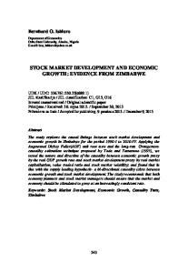
addition, all the estimated α’s in the four-factor model are not significantly different from zero at the 5% level, and the p-value of the GRS test is 0.596. Therefore, LMW significantly improves the performance of the three-factor model and helps to explain abnormal returns on extreme portfolios. Finally, the loadings on LMW are significantly different from zero at the 5% level except for the seventh portfolio, and are further away from zero when the prior returns become more extreme. Furthermore, the overreaction factor explains more than one-third (1.485×0.307=0.456) of the 1.215 spread in excess returns between the loser and the winner. This shows the explanatory power of LMW on stock returns and the fact that the extreme portfolios are subject to overreaction effect. To show the persistence of the overreaction effect, Panel B of Table VI shows the regression results for the winners, the losers, and their spreads in each of the five holding years.9 The qualitative results are very similar across the five holding years. First of all, HML accounts for most of the explanation in the three-factor model, but cannot explain all the abnormal returns. The spreads of the estimated α’s are significantly different from zero at the 5% level in the first, the fourth, and the fifth years. Secondly, the spreads of the estimated α’s are much smaller in the four-factor model and none of them are significantly different from zero at the 5% level. Furthermore, the loadings on LMW are significantly different from zero over the years. Therefore, the additional factor significantly improves the performance of the three-factor model in explaining abnormal returns on the extreme portfolios over the years. This also indicates that the overreaction effect is persistent over time. Finally, Figure 1 plots the return spread between the loser and the winner portfolios, and the shares of this spread that the four factors account for over the five holding years. It can be seen that the overreaction factor independent of SZ/BM and risk factors ( β LMW * LMW ) is not only persistent but also getting more important than the other three factors over the years. That is, the overreaction

9

Note that for holding years beyond the first one, HML and SMB are still formed by the returns

in the first year after portfolio formation. For example, the second-year return of the portfolio formed in 10/1980 is used to regress on HML and SMB formed in 10/1981.

14

independent of the fundamentals becomes more important than the fundamentals in explaining the abnormal returns after holding the portfolio for more than three years.

B. SZ/BM-based portfolios Given the correlations among SZ/BM, the factors, and overreaction, the returns on portfolios formed by their SZ and BM may contain both characteristics effects and overreaction effects. Including LMW in the factor model makes visible the overreaction effect embedded in returns on these portfolios. We first show the results for single-sorted SZ and BM portfolios. Panel A of Table VII shows regression results of the three-factor and the four-factor models for ten SZ-sorted portfolios. Panel B shows those for ten BM-sorted portfolios. Similar to previous studies, the HML loadings of BM-sorted portfolios are increasing with BM and the SMB loadings of SZ-sorted portfolios are decreasing with SZ. In the four-factor model, the LMW loadings are larger and significant for extreme portfolios, which confirms the existence of overreaction embedded in the returns on stocks with extreme SZ and BM. Comparing the overall performances of the three-factor and the four-factor models, we find that for the SZ-sorted portfolios in Panel A, the GRS test statistic is marginally significant at the 9.8% level in the three-factor model, and its p-value is higher at 13.1% in the four-factor model. For the BM-sorted portfolios in Panel B, both models perform well and the statistics of the GRS tests are both insignificant. For the spreads between the extreme portfolios, LMW helps to reduce the abnormal returns that cannot be explained by the three factors, but not as significantly as in the case of the winner/loser portfolios. Therefore, the additional factor can only marginally improve the performance of the three-factor model. Next, we turn to the double-sorted SZ/BM-based portfolios that are usually seen in the literature. Panel A of Table VIII reports the results of the three-factor model on the 5×5 SZ/BM-based portfolios constructed in Table I. In general, the patterns of the loadings on HML and SMB are similar to those in previous research. Within the same BM quintile, small firms tend to have a higher SMB loading, while within the same SZ quintile, high-BM firms tend to have a higher HML loading. Weak

15

firms tend to have high BM and therefore, have positive loadings on HML. On the other hand, strong firms tend to have low BM and negative loadings on HML. Small firms’ returns tend to have large loadings on SMB because they require extra compensation for their SZ. Panel B of Table VIII shows the results for the four-factor model. The results for loadings on HML, SMB, and MKT are very similar to those in the three-factor model and therefore, for brevity, are not shown here. Comparing Panels A and B, we find that first of all, in terms of the joint significance of abnormal returns, the GRS test shows that the null hypothesis that the intercepts are jointly zero is rejected at the 5% level in the three-factor model, while the test fails to reject the null at the 5% level in the four-factor model. Therefore, LMW improves the overall performance of the three-factor model. If we focus on the extreme portfolios, the contribution of the new factor becomes clearer. Panel C of Table VIII summarizes the statistics for the value (smallest SZ/highest BM) portfolio and the growth (biggest SZ/lowest BM) portfolio in the three-factor and the four-factor models. The additional factor LMW reduces the abnormal returns that cannot be explained by the three factors by about half. However, the new factor only accounts for about 16% of the spread of the abnormal returns between the value and the growth portfolios (1.142). In sum, for portfolio returns formed from sorts on SZ and/or BM, we conclude that the fourfactor model works better than the three-factor model. Due to the way we construct LMW, it is not surprising that the overreaction effects reported in this section are much weaker than those in the prior-return-based portfolios in the previous section. Nonetheless, in portfolios with extreme SZ and BM, we find significant overreaction in returns, which is consistent with the findings in Lakonishok, Shleifer, and Vishny (1994).

C. The four-factor model for the U.S. prior-return-based portfolios Fama and French (1996) show that their three-factor model can well explain the abnormal returns on the prior-return-based portfolios in the U.S. market. Therefore, it would be interesting to see how our four-factor model can improve the three-factor model in explaining the abnormal returns on the U.S. prior-return-based portfolios. We collect data on NYSE/AMEX/NASDAQ stocks for the period 1959-2001 from COMPUSTAT and CRSP. The portfolios are formed at the beginning of July 16

from 1964 to 1996. Table IX reports the regression results of the three-factor and the four-factor models using the U.S. data, comparable to Panel A of Table VI in the Japanese case. The top half of Table IX shows that the three-factor model describes the returns well in the prior-return-based portfolios. Almost all factor loadings are significantly different from zero at the traditional significance level. All the estimated abnormal returns (α’s) are insignificant. For the overall performance of the three-factor model, the null hypothesis that all the α’s in the prior-returnbased portfolios are jointly zero cannot be rejected at the traditional significance level (GRS P-value = 0.768). These results confirm the evidence shown in Fama and French (1996).10 Then what can the four-factor model do to improve the three-factor model? As in the Japanese case, the additional factor can help to explain the abnormal returns on the extreme portfolios. About 40% of the return from the loser-to-winner strategy still cannot be explained by the three factors. The spread of the estimated α’s between the loser and the winner portfolios is smaller if we add LMW as an additional factor, as shown in the bottom half of Table IX. The spread drops from 0.328 in the three-factor model to 0.241 in the four-factor model, i.e., LMW as an additional factor explains about 25% of the abnormal returns that cannot be explained by the three factors. The loadings on LMW are significantly different from zero at the 5% level except for the sixth portfolio. They are also further away from zero when the prior returns become more extreme. In addition, the overreaction factor explains more than one-third (2.065×0.134/0.740) of the spread in excess returns between the loser and the winner. This shows the explanatory power of LMW on stock returns and the fact that the extreme portfolios are subject to overreaction effect. Therefore, our argument is robust across different markets. 10

Fama and French’s (1996) portfolios are formed using returns for the four years from 60 to 13

months prior to portfolio formation. Since the momentum effect is not significant in Japan, we include the data from the first year prior to formation in the Japanese case. To be comparable, we use the same formation for the U.S. data, which, however, could only reduce the overreaction effect and strengthen our argument. In addition, since their portfolios are reformed monthly, they study the firstmonth returns after formation instead of the first-year returns after formation in our case. 17

IV. Conclusion Fama and French’s (1993) three-factor model successfully explains the abnormal returns on the characteristic-based portfolios in the U.S. market. Their risk factors are constructed by some characteristics of stocks. Daniel and Titman (1997) shows that this success is due to the high correlation between the factor loadings and the associated characteristics. Daniel, Titman, and Wei (2001) confirm Daniel and Titman’s (1997) argument in the Japanese market.

Therefore, they

conclude that the abnormal returns on the characteristic-based portfolios are directly related to their characteristics, not the Fama and French’s risk factors. On the other hand, using U.S. data, Fama and French (1996) show that their three-factor model can also well explain the abnormal returns on the prior-return-based portfolios, which reflect the overreaction of the investors. This motivates us to further investigate whether characteristics can also explain the abnormal returns on the prior-returnbased portfolios. We focus on the Japanese market because it is argued that overreaction is stronger in Japan than in the U.S. due to the institutional structure in the Japanese market. Through comparisons of the returns on the SZ/BM-based and the prior-return-based portfolios, we explicitly point out that some return patterns in the prior-return-based portfolios cannot be explained by the characteristics.

Therefore, even though Daniel, Titman, and Wei’s (2001)

characteristic hypothesis can explain the success of the three-factor model, there exists, other than the characteristics and risk factors, another factor that may explain the expected stock return.

As

suggested by De Bondt and Thaler (1985, 1987), Chopra et al (1992), and Lakonishok, Shleifer, and Vishny (1994), overreaction plays an important role in abnormal returns. In an attempt to isolate the overreaction effects from the SZ/BM effects, we construct the SZ/BM-adjusted returns for the prior-return-based portfolios by subtracting a benchmark return formed on their SZ and BM from the portfolios’ average returns. We find that this overreaction effect after controlling for SZ/BM is not only significant, but also persistent in the prior-return-based portfolios. Motivated by the potential importance of overreaction after controlling for the SZ/BM effects, we propose a new factor, called LMW, to mimic the overreaction effect in returns. LMW is the SZ/BM-adjusted zero-investment return on the 30% loser to the 30% winner orthogonal to HML and 18

SMB. We find remarkable explanatory power of this new factor on the abnormal returns on several prior-return-based and characteristics-based portfolios. Moreover, the additional factor improves the performances of the three-factor model. Finally, we apply the four-factor model to the U.S. data and find consistent results. This shows the robustness of our arguments across different markets. It is instructive to mention that we do not attempt to dispute Daniel, Titman, and Wei (2001)’s explanation on the success of the three-factor model in the characteristic-based portfolios. Instead, we suggest that the overreaction effect be explicitly considered.

The difference between the

characteristics model and the risk factor model is the explanation on the factor loadings. By adding a new factor to the three-factor model, we are not involved in the battle of the explanation on the factor loadings. Instead, our new factor is independent of both characteristics and the original three risk factors. This paper only discusses two of the firm characteristics, SZ and BM, and attributes the returns that are independent of SZ, BM, and risk factors to overreaction. This knife-edge distinction may not be proper because our defined overreaction may contain effects from other characteristics such as cash flow and sales. We make this simplified assumption because many papers in the literature conclude that SZ and BM are the two most significant firm characteristics in explaining stock returns.11 Future extensions include attempts to separate the overreaction from effects of other characteristics.

11

We also experiment the SZ/Cash flow and the SZ/Earning per share double-sorted portfolios.

The return patterns on these portfolios are not as clear as that of the SZ/BM sorted portfolios.

19

Reference Carhart, M.M., 1997. On Persistence in Mutual Fund Performance, Journal of Finance 52, 57-82. Chan, L.K.C., Y. Hamao, and J. Lakonishok, 1991. Fundamentals and Returns in Japan, Journal of Finance, 46, 1739-1764. Chan, L.K.C., N. Jegadeesh, and J. Lakonishok, 1996. 51, 1681-1713.

Momentum Strategies, Journal of Finance,

Chang, R.P., D.W. McLeavey, and S.G. Rhee, 1995. Short-Term Abnormal Returns of the Contrarian Strategy in the Japanese Stock Market, Journal of Business Finance and Accounting, 22, 1035-1048. Chopra, N., J. Lakonishok and J.R. Ritter, 1992. Measuring Abnormal Performance, Journal of Financial Economics, 31, 235-268. Chui, A.C.W., S. Titman, and K.C.J. Wei, 2000. Momentum, Legal Systems and Ownership Structure: An Analysis of Asian Stock Markets, Working paper, Hong Kong University of Science and Technology. Daniel, K. and S. Titman, 1997. Evidence on the Characteristics of Cross Sectional Variation in Stock Returns, Journal of Finance, 52, 1-33. Daniel, K., S. Titman, J.K.C. Wei, 2001. Explaining the Cross-Section of Stock Returns in Japan: Factors or Characteristics? Journal of Finance, 56, 743-766. De Bondt, W.F.M. and R. Thaler, 1985. Does The Stock Market Overreact? Journal of Finance, 40, 793-805. De Bondt, W.F.M. and R. Thaler, 1987. Further Evidence on Investor Overreaction and Stock Market Seasonality, Journal of Finance, 42, 557-581. Fama, E.F. and K.R. French, 1992. The Cross-Section of Expected Stock Returns, Journal of Finance, 47, 427-465. Fama, E.F. and K.R. French, 1993. Common Risk Factors in The Returns on Stocks and Bonds, Journal of Financial Economics, 33, 3-56. Fama, E.F. and K.R. French, 1996. Multifactor Explanations of Asset Pricing Anomalies, Journal of Finance, 51, 55-84. Gibbons, M.R., S. Ross, and J. Shanken, 1989. A Test of the Efficiency of a Given Portfolio, Econometrica, 57, 1121-1152.

Gunaratne, P.S.M., 1996. Effect of the Length of the Ranking Period over the Performance of the Post-Ranking Period: A Test of Investor Overreaction in Tokyo Stock Exchange, Journal of Financial Management and Analysis, 9, 66-73. Gunaratne, P.S.M., Y. Yonesawa, 1997. Return Reversals in the Tokyo Exchange: A Test of Stock Market Overreaction, Japan and the World Economy, 9, 363-384. Jegadeesh, N. and S. Titman, 1993, Returns to Buying Winners and Selling Losers: Implications for Stock Market efficiency, Journal of Finance, 48, 65-91.

20

Lakonishok, J., A. Shleifer, and R. Vishny, 1994. Contrarian Investment, Extrapolation, and Risk, Journal of Finance, 49, 1541-1578. La Porta, R., J. Lakonishok, A. Shleifer, and R. Vishny, 1997. Good News for Value Stocks: Further Evidence on Market Efficiency, Journal of Finance, 52, 859-874.

21

Figure 1: Decomposition of the yearly average returns of the loser-to-winner portfolio This figure plots the return spread between the loser and the winner portfolios (Loser – Winner), and the shares of this spread that the four factors account for ( β HML * HML, β SMB * SMB, β MKT * MKT , and β LMW * LMW ) over the five holding years.

1.4

Loser - Winner Beta_HML*HML Beta_SMB*SMB Beta_MKT*MKT Beta_LMW*LMW

1.2

Return (%)

1 0.8 0.6 0.4 0.2 0 -0.2 1

2

3 Year after formation

22

4

5

Table I: Average monthly returns, BM, and SZ of the 5×5 (25) SZ/BM-sorted portfolios over the first year after portfolio formation A portfolio’s BM for formation year t is the sum of book equity for the firms in the portfolio for the fiscal year ending in calendar year t-1 divided by the sum of their SZ in December of year t-1. A portfolio’s SZ is the average of logarithms of market equity for the firms in the portfolio in September of year t. At the beginning of each October from 1980 to 1994, all TSE stocks in our sample are sorted into five equal groups, from small to large, based on their SZ. We also independently divide all TSE stocks into five equal BM groups from low to high. The 25 SZ/BM-sorted portfolios are constructed from the intersections of these five SZ and five BM groups. Once formed, the 25 portfolios are held for one year. The returns on these portfolios are equally weighted.

Low Small 2 SZ 4 Big

1.586 0.978 0.413 0.654 0.423

Small 2 SZ 4 Big

7.659 6.879 6.668 6.768 6.174

Small 2 SZ 4 Big

8.988 10.016 10.720 11.539 13.569

Small 2 SZ 4 Big

0.226 0.240 0.239 0.238 0.227

2

BM Returns 1.534 1.745 1.278 1.400 0.864 0.957 0.774 0.887 0.879 0.950 Standard deviations 7.266 7.072 7.145 6.956 6.560 6.242 6.350 5.887 5.956 5.645 Average ln(SZ) 8.989 9.073 10.007 10.037 10.735 10.742 11.542 11.569 13.379 13.188 Average BM 0.359 0.460 0.369 0.464 0.367 0.469 0.367 0.456 0.359 0.444

23

4

High

1.620 1.362 1.047 1.036 1.205

1.761 1.461 1.391 1.104 1.409

6.844 6.575 6.431 5.350 5.688

6.700 6.438 6.211 6.058 6.426

9.060 10.031 10.741 11.583 13.112

9.131 10.022 10.770 11.549 13.035

0.567 0.581 0.576 0.570 0.537

0.799 0.782 0.754 0.724 0.692

Table II: Average monthly returns, BM, and SZ of the matching winner and the matching loser portfolios At the beginning of each October between 1980 and 1994, all TSE stocks in our sample are sorted based on their prior five-year cumulative returns. The top N1 stocks with the highest cumulative returns are used to form the “matching winner” portfolio, where N1 is the number of firms in the Big-SZ/LowBM portfolio in Table I. The bottom N2 stocks with the lowest cumulative returns are used to form the “matching loser” portfolio, where N2 is the number of firms in the Small-SZ/High-BM portfolio in Table I. That is, the numbers of stocks included in the matching winner and the matching loser portfolios respectively match the numbers of stocks included in the two extreme SZ-BM-based portfolios on the same reformation dates. Once formed, these portfolios will be held for five years, during which the numbers of including stocks are unchanged. The returns on these portfolios are equally weighted. For comparison, at the bottom of the Table we report the statistics of these two extreme SZ-BM-based portfolios Panel A Holding Year

1st 2nd 3rd 4th 5th

Zero-investment portfolio of matching loser-to-matching winner Return Standard Average Average Non-January Return Standard Average Average Non-January Return Difference in Difference in Non-January deviation ln(SZ) BM Return deviation ln(SZ) BM Return Average ln(SZ) Average BM Return 1.545 1.881 1.059 0.861 1.362

6.802 7.203 7.243 7.972 8.307

11.404 11.563 11.662 11.723 11.817

0.612 0.559 0.520 0.566 0.587

Value (smallest-SZ/highest-BM) portfolio

1st

Panel B

Matching loser

Matching winner

1.408 1.677 0.808 0.460 1.023

0.129 0.451 0.342 0.010 0.130

6.310 6.522 7.122 7.438 7.630

12.030 11.997 11.957 11.915 11.881

0.254 0.317 0.362 0.428 0.506

-0.079 0.262 0.230 -0.298 -0.174

Growth (Largest-SZ/Lowest-BM) portfolio

1.416** 1.430** 0.718** 0.851** 1.231**

-0.627 -0.434 -0.295 -0.192 -0.064

0.358 0.242 0.158 0.139 0.081

1.487** 1.415** 0.577 0.758** 1.196**

Zero-investment portfolio of value-to-growth Return Standard Average Average Non-January Return Standard Average Average Non-January Return Difference in Difference in Non-January deviation ln(SZ) BM Return deviation ln(SZ) BM Return Average ln(SZ) Average BM Return 1.761 6.700 9.131 0.799 1.600 0.423 6.174 13.569 0.227 0.238 1.338** -4.438 0.572 1.362**

The asterisk ** indicates significance of portfolio returns at the 5% level.

24

Table III: Percentages (%) of firms in the matching winner and loser portfolios located in each of the 5×5 current-year SZ-BM sorted portfolios

Low

Matching Loser 2 BM 4

High

Sum

Low

Matching Winner 2 BM 4

High

Sum

Year 1 Small 2 SZ 4 Large Sum

3.47 2.62 3.37 3.99 8.76 22.22 2.30 3.12 3.84 4.22 9.88 23.35 1.03 2.31 3.08 6.03 10.07 22.52 0.70 0.78 3.37 3.49 9.73 18.07 0.98 2.27 2.12 3.37 5.11 13.85 8.47 11.10 15.78 21.10 43.55 100.00

11.32 4.56 12.80 3.36 14.78 5.13 11.02 3.52 17.43 2.83 67.34 19.40

2.49 2.16 1.79 1.06 0.86 8.37

1.42 0.96 0.47 0.34 0.35 3.54

0.52 0.33 0.19 0.30 0.00 1.35

20.31 19.62 22.35 16.25 21.47 100.00

10.73 5.81 3.15 9.50 4.93 2.54 8.50 6.00 3.05 8.55 3.80 1.87 13.40 3.83 1.37 50.70 24.37 11.98

3.08 1.53 2.42 1.12 0.79 8.95

2.20 0.85 0.37 0.49 0.09 4.00

24.97 19.36 20.35 15.82 19.49 100.00

9.24 5.80 4.14 4.08 6.63 6.03 3.79 2.29 6.48 4.87 4.29 3.09 7.00 3.39 1.96 2.04 10.42 4.24 2.70 0.47 39.77 24.33 16.87 11.96

3.69 1.52 0.70 0.89 0.28 7.08

26.94 20.26 19.42 15.28 18.10 100.00

9.35 6.06 4.95 4.78 4.38 6.54 4.57 4.59 3.10 2.64 5.19 4.00 4.12 2.99 1.65 4.75 3.39 2.54 1.73 1.39 8.48 4.86 2.53 0.98 0.45 34.32 22.87 18.73 13.58 10.51

29.52 21.44 17.95 13.80 17.29 100.00

9.66 5.84 5.41 5.54 5.88 4.83 4.73 4.00 3.79 3.47 4.29 4.48 3.44 4.31 2.49 3.71 1.98 3.07 1.72 1.64 6.72 4.83 2.48 1.52 0.17 29.21 21.86 18.39 16.88 13.66

32.33 20.82 19.00 12.12 15.73 100.00

Year 2 Small 2 SZ 4 Large Sum

3.99 2.75 3.06 4.89 6.35 3.34 3.02 3.64 4.00 8.29 1.76 3.25 3.98 5.87 8.30 1.44 2.18 3.00 4.35 7.51 1.32 3.32 2.24 4.02 4.13 11.85 14.52 15.92 23.14 34.57

Small 2 SZ 4 Large Sum

4.41 2.74 3.77 4.75 5.00 4.73 2.59 3.55 4.04 6.96 2.51 4.04 4.71 5.79 6.76 1.67 2.75 3.55 4.51 5.73 2.58 3.76 3.23 2.56 3.31 15.90 15.88 18.81 21.65 27.76

Small 2 SZ 4 Large Sum

4.18 4.41 2.05 4.02 4.63 5.92 3.95 3.86 3.76 6.45 2.66 4.27 5.06 3.93 6.69 2.40 2.60 4.35 4.26 5.50 2.83 3.53 3.79 1.83 3.08 18.00 18.74 19.12 17.80 26.34

Small 2 SZ 4 Large Sum

5.50 3.80 3.62 2.42 3.65 5.02 3.92 3.85 3.89 6.39 3.23 4.88 4.92 4.38 4.52 2.89 3.74 4.80 4.00 5.17 3.63 3.55 3.25 2.51 2.48 20.27 19.89 20.44 17.20 22.21

21.04 22.29 23.16 18.47 15.04 100.00

Year 3 20.66 21.87 23.81 18.22 15.44 100.00

Year 4 19.29 23.93 22.61 19.11 15.05 100.00

Year 5 18.99 23.07 21.92 20.61 15.41 100.00

25

Table IV: Average SZ/BM-adjusted returns on the matching winner and the matching loser For each stock in the portfolio, replace its return in each month with the monthly return on the SZ/BM-based portfolio where its SZ and BM are located (one of the 5×5 constructed in Table I). Then equally weight these returns across all stocks in the original portfolio and call it the benchmark return. The monthly SZ/BM-adjusted return on the original portfolio is then computed as the average return on that portfolio minus the benchmark return. Therefore, the SZ/BM-adjusted return of a firm is its return in excess of a benchmark return formed on its SZ and BM. Matching Loser

Matching Winner

Zero-investment (Matching loser-to-winner) SZ/BM-adjusted Unadjusted SZ/BM-adjusted Unadjusted SZ/BM-adjusted Unadjusted returns returns returns returns returns returns 1st 0.099 1.545** -0.583** 0.129 0.682** 1.416** 2nd 0.385** 1.881** -0.633** 0.451 1.019** 1.430** 3rd -0.292 1.059* -0.410** 0.342 0.118 0.718** 4th -0.093 0.861 -0.515** 0.010 0.422* 0.851** 5th 0.263 1.362** -0.588** 0.130 0.852** 1.231** The asterisks * and ** indicate significance of portfolio returns at the 10% and 5% level, respectively.

26

Table V: Means, standard deviations, and correlation coefficients of the factors This table reports the means and the standard deviations of MKT, HML, and SMB over the first 12 months after portfolio formation, and those of LMW’ and LMW over the 12 months of each year of the five-year holding periods. The associated portfolios constructing these factors are reformed annually from 10/1980 to 09/1994. The factors HML and SMB are defined in Table IV and MKT is the value-weighted average market return. The factor LMW’ and LMW are constructed as follows. At the beginning of each October from 1980 to 1994, all TSE stocks are allocated to three groups [the bottom 30 percent (the loser), middle 40 percent, and top 30 percent (the winner)] based on their prior 60-month cumulative monthly returns. Once formed, the portfolios are held for five years. Those 60 monthly returns of each stock in the winner and the loser portfolios are adjusted for SZ and BM in the same way as we do in Table IV. Then we form the zero-investment loser-to-winner portfolio by taking the difference of the SZ/BM-adjusted returns between the winner and the loser portfolios. LMW’ is this difference. We then regress LMW’ on HML and SMB. The sum of the intercept and the residual from the regression yields LMW. Therefore, LMW is orthogonal to HML and SMB. Panel A: Means and standard deviations Factor HML SMB MKT LMW’ LMW

Mean 0.618 0.233 0.882 0.455 0.307

Year 1 Standard deviation 2.643 4.379 5.751 2.093 1.915

Mean

Year 2 Standard deviation

Mean

Year 3 Standard deviation

Mean

Year 4 Standard deviation

Mean

Year 5 Standard deviation

0.530 0.311

1.949 1.709

0.275 0.147

2.102 2.019

0.412 0.309

1.960 1.914

0.489 0.390

1.847 1.793

Panel B: Correlation coefficients Year 1 Factor HML SMB MKT LMW’ HML 1.000 SMB 0.071 1.000 MKT -0.209 -0.170 1.000 LMW’ 0.253 0.332 -0.061 1.000

Year 2 HML SMB MKT LMW’ 1.000 0.096 1.000 -0.217 -0.150 1.000 0.461 0.183 0.172 1.000

Year 3 HML SMB MKT LMW’ 1.000 0.082 1.000 -0.221 -0.106 1.000 0.278 0.010 0.224 1.000

27

Year 4 HML SMB MKT LMW’ 1.000 0.106 1.000 -0.205 -0.041 1.000 0.210 0.074 0.211 1.000

Year 5 HML SMB MKT LMW’ 1.000 0.114 1.000 -0.157 0.017 1.000 0.204 -0.100 0.277 1.000

Table VI: Three-factor and four-factor regressions for returns on ten prior-return-based portfolios The portfolios are formed and ranked according to their prior five-year cumulative returns. The results are from the following regressions: Three-factor model:

Ri ,t − R f ,t = α i + β i , HML HMLt + β i , SMB SMBt + β i , MKT MKTt + ε i ,t ,

Four-factor model:

Ri ,t − R f ,t = α i + β i , HML HMLt + β i ,SMB SMBt + β i , MKT MKTt + β i , LMW LMWt + ε i ,t ,

where Ri,t is the return of portfolio i and Rf,t is the risk-free return defined in Section II. The factors are defined in Table V. GRS is the F-statistic proposed by Gibbons, Ross, and Shanken (1989) to test the joint hypothesis that the regression intercepts for a set of ten portfolios are all zero. The p-value of GRS is denoted as p(GRS). t(⋅) is the t-statistic. Panel A: Full results for the first year returns

Excess Return

Loser

2

3

4

5

6

7

8

1.101

1.080

1.034

0.962

0.893

0.817

0.728

0.615

0.326

0.235 0.289 0.737 0.976

0.203 0.228 0.739 0.971

0.145 0.220 0.675 0.990

0.110 0.152 0.687 0.986

0.088 0.022 0.694 1.011

0.007 -0.029 0.678 1.017

-0.205 -0.130 0.654 0.998

Three-factor regressions 0.165 0.281 α (%) HML SMB MKT t(α) t(HML) t(SMB) t(MKT)

0.435 0.855 1.017

0.313 0.763 0.932

9 Winner

LoserWinner Spread -0.114 1.215

-0.440 -0.393 0.615 0.926

0.605 0.828 0.241 0.091

1.207 2.364 2.160 2.024 1.457 1.288 1.081 0.076 -1.864 -2.697 2.385# 8.496 7.036 7.114 6.072 5.917 4.773 0.729 -0.847 -3.172 -6.446 8.725# 27.879 28.646 30.243 32.905 30.254 36.015 38.052 32.793 26.562 16.819 4.230# 42.755 45.113 51.649 55.770 57.248 66.630 71.496 63.423 52.308 32.673 2.066#

p(GRS) = 0.380

Four-factor regressions -0.038 0.111 α (%) HML SMB MKT LMW t(α) t(HML) t(SMB) t(MKT) t(LMW)

-0.205 -0.388 0.617 0.939 -0.796

0.168 0.818 0.236 0.067 1.485

-0.406 1.323 1.049 1.128 0.779 0.720 0.996 0.922 -0.733 -1.795 12.537 9.947 9.897 7.076 6.298 4.959 0.725 -0.867 -4.074 -9.153 41.487 40.925 42.509 38.708 32.417 37.678 38.073 35.677 35.115 24.332 63.021 63.891 72.057 65.244 61.102 69.492 71.441 69.113 69.451 47.671 14.859 13.758 13.316 8.361 5.213 4.166 0.500 -5.705 -11.535 -13.911

1.294# 17.050# 8.198# 2.999# 22.912#

0.430 0.853 1.006 0.689

0.309 0.761 0.922 0.577

0.082 0.286 0.735 0.967 0.519

0.097 0.225 0.738 0.966 0.359

0.073 0.219 0.674 0.986 0.244

0.059 0.151 0.687 0.983 0.171

0.082 0.022 0.694 1.010 0.021

0.079 -0.028 0.679 1.021 -0.245

-0.062 -0.127 0.655 1.006 -0.485

p(GRS)=0.596

# These values are the t-statistic for the null hypothesis that the spread is zero. They are not the spreads between the t-statistics.

28

Panel B: Regression results for the winner, the loser, and their spread for five holding years

Excess Return

Loser 1.101

1st Year Winner L-W Spread -0.114 1.215

Three-Factor Model 0.165 -0.440 α (%) HML 0.435 -0.393 SMB 0.855 0.615 MKT 1.017 0.926 t(α) t(HML) t(SMB) t(MKT)

1.207 8.496 27.879 42.755

Four-Factor Model -0.038 α (%) HML 0.430 SMB 0.853 MKT 1.006 LMW 0.689 t(α) t(HML) t(SMB) t(MKT) t(LMW)

-2.697 -6.446 16.819 32.673 -0.205 -0.388 0.617 0.939 -0.796

-0.406 -1.795 12.537 -9.153 41.487 24.332 63.021 47.671 14.859 -13.911

0.605 0.828 0.241 0.091

Loser 1.332

2nd Year Winner L-W Spread 0.237 1.095

0.144 0.553 0.839 1.062

-0.256 -0.445 0.779 0.888

0.400 0.998 0.060 0.174

2.385# 1.243 8.725# 12.596 4.230# 31.777 2.066# 53.263

-1.694 -7.774 22.657 34.207

1.857# 12.236# 1.224# 4.695#

-0.059 -0.403 0.795 0.980 -0.883

0.080 0.930 0.033 0.023 1.435

1.294# 0.221 -0.558 17.050# 14.788 -10.137 8.198# 38.747 33.355 2.999# 58.402 51.164 22.912# 9.744 -13.968

0.646# 19.978# 1.194# 1.040# 19.387#

0.168 0.818 0.236 0.067 1.485

0.021 0.527 0.828 1.004 0.552

3rd Year Loser Winner L-W Spread 0.753 0.105 0.648

-0.068 0.344 0.819 1.055

-0.265 -0.306 0.831 0.882

-0.501 -1.456 6.690 -4.441 27.745 20.989 45.957 28.654 -0.111 0.311 0.811 0.985 0.644

-0.201 -0.256 0.844 0.985 -0.958

-1.146 -1.754 8.444 -5.898 38.464 33.848 57.293 48.432 13.171 -16.576

0.197 0.650 -0.012 0.173

Loser 0.579

4th Year 5th Year Winner L-W Spread Loser Winner L-W Spread -0.175 0.754 0.922 -0.032 0.954

0.103 0.221 0.858 1.051

-0.356 -0.185 0.835 0.903

0.732# 0.797 6.376# 4.531 -0.202# 33.375 3.797# 49.994

-2.147 -2.949 25.246 33.374

0.090 0.567 -0.033 0.001 1.602

-0.038 0.200 0.856 1.006 0.527

-0.103 -0.147 0.837 0.984 -0.950

0.699# -0.356 -1.052 11.620# 5.009 -3.973 -1.171# 40.884 43.213 0.025# 56.560 59.864 24.697# 9.533 -18.564

0.459 0.406 0.023 0.148

0.255 0.337 0.854 1.070

-0.352 -0.103 0.875 0.906

0.607 0.044 -0.021 0.164

1.989# 1.833 4.651# 6.480 0.494# 30.905 3.936# 48.162

-2.315 -1.814 28.934 37.232

2.670# 5.174# -0.474# 4.519#

-0.057 -0.071 0.872 0.990 -0.871

0.133 0.388 -0.016 0.030 1.401

0.665# 0.616 -0.561 9.360# 7.035 -1.888 0.995# 35.758 43.572 1.294# 50.095 58.195 28.783# 7.733 -15.218

0.973# 7.723# -0.589# 1.308# 18.338#

0.066 0.346 0.019 0.021 1.477

# These values are the t-statistic for the null hypothesis that the spread is zero. They are not the spreads between the t-statistics.

29

0.075 0.317 0.856 1.019 0.530

Table VII: Three-factor and four-factor regressions for returns on ten SZ-sorted and ten BMsorted portfolios See the notes in Table VI. The portfolios are formed as follows. At the beginning of each October from 1980 to 1998, all TSE stocks in our sample are sorted into ten equal groups, from small to large, based on their most recent SZ (in Panel A), and from low to high, based on their year-end BM (in Panel B). Once formed, the portfolios are held for one year. The returns on these portfolios are equally weighted. Panel A: ten SZ-sorted portfolios Excess Returns

1 (Small)

2

3

4

5

6

7

8

1.191

0.856

0.662

0.618

0.393

0.307

0.317

0.369

0.349

0.444

1-10 spread 0.747

0.029 0.234 1.041 1.007

0.011 0.206 0.978 1.007

-0.170 0.174 0.883 1.009

-0.250 0.197 0.770 0.970

-0.156 0.128 0.578 0.955

-0.112 0.126 0.418 0.932

-0.065 0.042 0.230 0.970

0.049 0.047 -0.118 0.969

0.555 0.220 1.395 -0.046

Three-factor regressions 0.604 0.257 α (%) HML SMB MKT t(α) t(HML) t(SMB) t(MKT) p(GRS)

0.267 1.277 0.923

0.208 1.171 0.967

3.103 2.520 0.391 0.182 -2.632 -2.898 -1.608 -1.070 -0.651 0.933 2.875# 3.448 5.153 8.036 8.594 6.771 5.761 3.325 3.025 1.069 2.252 2.869# 30.915 54.185 66.951 76.345 64.461 42.136 28.001 18.755 10.876 -10.670 34.021# 27.595 55.261 80.016 97.101 90.988 65.525 57.178 51.662 56.673 108.482 -1.389# 0.098

Four-factor regressions 0.532 0.135 α (%) HML SMB MKT LMW t(α) t(HML) t(SMB) t(MKT) t(LMW) p(GRS)

9 10 (big)

0.032 0.045 -0.118 0.967 0.050

0.500 0.216 1.395 -0.055 0.172

2.734 1.285 0.277 -0.411 -2.706 -3.320 -1.772 -1.340 -0.913 0.622 3.424 5.135 8.022 8.763 6.757 5.775 3.302 2.996 1.028 2.216 31.297 54.412 67.025 78.823 64.525 42.797 28.083 18.885 10.945 -10.766 27.273 54.662 79.093 98.556 89.948 65.410 56.528 51.175 56.145 107.897 2.329 2.154 0.695 3.779 0.660 2.620 1.137 1.752 1.688 1.948

2.575# 2.838# 34.276# -1.655# 1.812#

0.262 1.277 0.911 0.222

0.207 1.171 0.963 0.168

0.021 0.233 1.041 1.006 0.025

-0.024 0.204 0.978 1.001 0.109

-0.177 0.173 0.883 1.008 0.021

-0.285 0.195 0.770 0.964 0.110

-0.174 0.127 0.578 0.952 0.055

-0.141 0.124 0.418 0.927 0.090

-0.091 0.040 0.230 0.965 0.083

0.131

# These values are the t-statistic for the null hypothesis that the spread is zero. They are not the spreads between the t-statistics.

30

Panel B: ten BM-sorted portfolios Excess Returns

1 (Low)

2

3

4

5

6

7

8

9

0.188

0.319

0.387

0.509

0.574

0.560

0.654

0.689

0.005 -0.103 0.678 0.978

0.025 0.055 0.645 0.961

0.051 0.144 0.686 0.967

0.029 0.210 0.671 0.946

0.062 0.277 0.675 0.955

0.020 0.446 0.669 0.957

Three-factor regressions -0.085 0.025 α (%)

10-1 spread 0.689

0.032 0.522 0.725 0.993

0.027 0.737 0.842 1.028

0.112 1.132 -0.091 0.050

HML SMB MKT

-0.395 0.933 0.978

t(α) t(HML) t(SMB) t(MKT)

-0.728 0.310 0.073 0.302 0.658 0.418 0.970 0.333 0.456 -8.490 -8.133 -3.582 1.666 4.707 7.641 10.877 18.542 18.731 37.548 40.801 44.197 36.655 41.867 45.725 49.656 52.043 48.701 48.581 67.479 78.824 67.511 72.819 79.670 86.815 91.984 82.324

p(GRS)

-0.264 0.706 0.946

0.744

10 (High) 0.877

0.992

Four-factor regressions -0.004 0.017 α (%) -0.264 0.706 0.945 0.027

0.005 -0.103 0.678 0.978 0.002

0.007 0.054 0.645 0.958 0.055

0.019 0.142 0.686 0.961 0.099

0.003 0.208 0.670 0.942 0.079

0.046 0.276 0.675 0.953 0.049

0.017 0.446 0.669 0.957 0.010

-0.005 0.520 0.725 0.987 0.114

HML SMB MKT LMW

-0.401 0.933 0.965 -0.241

t(α) t(HML) t(SMB) t(MKT) t(LMW)

-0.600 0.202 0.065 0.088 0.246 0.050 0.716 0.278 -0.070 -8.969 -8.157 -3.582 1.634 4.705 7.667 10.890 18.530 19.114 39.132 40.841 44.197 36.805 42.524 46.293 49.935 52.055 49.961 49.416 66.683 77.923 66.820 72.737 79.401 86.082 90.915 82.998 -4.323 0.665 0.049 1.339 2.623 2.331 1.567 0.325 3.371

p(GRS)

0.280 0.760# 19.521 19.340# 41.755 -2.937# 62.999 1.987#

-0.024 0.733 0.841 1.020 0.158

-0.260 -0.187# 19.944 19.423# 42.881 -2.944# 63.454 2.142# 3.444 5.578#

0.997

# These values are the t-statistic for the null hypothesis that the spread is zero. They are not the spreads between the t-statistics.

31

-0.020 1.134 -0.092 0.055 0.399

Table VIII: Three-factor and four-factor regressions for returns on 25 SZ/BM-sorted portfolios See Table I for portfolio construction and the notes in Table VI for definitions of the notations. The statistics for loadings in HML, SMB, and MKT in the four-factor model are very similar to those in the three-factor model and therefore, for brevity, are omitted in the Table. Panel A : Three-factor regression Size

Low

2

BM

4

High

Low

2

0.370 0.133 -0.291 -0.036 0.040

0.385 0.026 -0.053 -0.262 -0.229

2.607 -0.593 -3.482 -0.304 -0.536

2.079 -0.353 -0.720 -1.836 0.468

0.284 0.274 0.462 0.257 0.549

0.554 0.631 0.632 0.641 0.699

-1.003 -3.546 -6.578 -5.024 -12.763

1.655 1.305 -1.629 -0.612 -2.557

1.133 0.956 0.764 0.428 0.049

1.127 0.901 0.763 0.493 0.094

32.034 36.879 31.202 15.524 5.113

32.481 42.387 30.507 18.996 1.286

0.902 0.982 1.021 0.888 0.976

0.908 1.020 1.026 1.007 1.037

32.034 36.879 31.202 15.524 5.113

32.481 42.387 30.507 18.996 1.286

t(HML) 3.603 4.579 3.910 1.611 5.585 t(SMB) 34.242 44.043 37.260 18.247 3.037 t(MKT) 34.242 44.043 37.260 18.247 3.037

0.328 0.109 -0.301 -0.050 0.035

0.326 0.007 -0.099 -0.317 -0.266

2.237 -1.218 -2.636 0.488 0.505

2.009 -0.476 -0.630 -1.949 0.036

0.132 0.072 0.031 0.046 0.018

0.183 0.058 0.143 0.170 0.116

3.991 2.471 0.002 -4.001 -4.155

0.283 0.805 -0.519 0.838 2.752

α (%) Small 2 SZ 4 Big

0.534 -0.090 -0.488 -0.056 -0.056

Small 2 SZ 4 Big

-0.082 -0.214 -0.366 -0.370 -0.526

Small 2 SZ 4 Big

1.393 1.191 0.927 0.610 0.113

Small 2 SZ 4 Big

1.005 0.987 0.967 0.945 0.952

0.382 0.549 -0.042 0.044 -0.092 -0.222 -0.250 -0.101 0.046 -0.032 p(GSR) =0.025 HML 0.121 0.230 0.061 0.200 -0.083 0.168 -0.033 0.082 -0.099 0.222 SMB 1.265 1.167 1.064 1.025 0.826 0.856 0.549 0.494 0.027 0.064 MKT 0.942 0.934 1.043 1.005 0.991 0.951 0.992 0.932 0.969 0.974

Panel B: Four-factor regression α (%) Small 2 SZ 4 Big

0.440 -0.130 -0.424 0.042 0.075

Small 2 SZ 4 Big

0.291 0.123 0.000 -0.308 -0.408

0.373 0.536 -0.057 0.088 -0.081 -0.249 -0.268 -0.166 0.003 -0.104 p(GSR) =0.082 LMW 0.026 0.041 0.047 -0.136 -0.033 0.085 0.056 0.202 0.181 0.223

32

BM t(α) 3.423 0.399 -2.050 -0.789 -0.316

4

High

2.157 1.448 -3.154 -0.368 0.409

2.320 0.304 -0.495 -2.024 -1.215

4.170 7.516 12.593 6.665 13.982

8.389 18.874 14.826 12.457 9.357

31.094 49.170 38.966 20.763 2.322

31.960 50.493 33.540 17.921 2.342

31.094 49.170 38.966 20.763 2.322

31.960 50.493 33.540 17.921 2.342

t(α) 3.302 0.800 -2.287 -1.316 -1.073

1.898 1.186 -3.224 -0.514 0.345

2.016 0.082 -0.930 -2.457 -1.401

t(LMW) 0.512 -2.533 1.590 3.281 4.722

2.374 1.601 0.674 0.949 0.371

2.814 1.393 2.740 2.693 1.247

Panel C: Extreme portfolios Three-factor model Value portfolio Growth portfolio Spread Four-factor model Value portfolio Growth portfolio Spread

Excess Return

α

MKT

HML

SMB

1.231 0.089 1.142

0.385 -0.056 0.441

0.908 0.952 -0.044

0.554 -0.526 1.080

1.127 0.113 1.014

1.231 0.089 1.142

0.326 0.075 0.251

0.904 0.952 -0.048

0.552 -0.526 1.078

1.127 0.113 1.014

33

LMW

0.183 -0.408 0.591

Table IX: Three-factor and four-factor regressions for the first year returns on ten priorreturn-based portfolios in the U.S. market See the notes in Table VI. The constructions of the factors are similar to those in the Japanese case, with an exception that in the U.S. the portfolios are reformed in July instead of October. The definitions of BM and SZ are identical to those applied by Fama and French (1993).

Loser

2

3

4

5

6

7

8

0.895

0.833

0.826

0.867

0.754

0.778

0.671

0.434

0.740

0.092 0.445 0.889 0.853

0.043 0.398 0.840 0.881

0.097 0.295 0.758 0.869

0.153 0.227 0.767 0.883

0.044 0.174 0.757 0.916

0.116 0.027 0.793 0.902

0.022 -0.120 0.823 0.961

-0.186 -0.381 0.954 1.016

0.328 1.037 0.528 -0.137

0.629 -0.119 0.734 0.364 0.914 1.411 0.395 1.009 0.174 -1.265 8.982 11.032 11.011 10.363 8.590 6.476 4.851 0.732 -2.975 -8.030 24.919 25.930 26.994 26.883 27.104 26.906 25.939 26.246 25.057 24.686 20.598 30.286 36.150 39.322 43.307 43.222 43.757 41.637 40.800 36.661

1.726# 12.674# 7.929# -2.871#

Excess Return 1.174 0.878 Three-factor regressions α (%) 0.142 -0.018 β HML 0.656 0.552 β SMB 1.483 1.057 β MKT 0.879 0.885 t(α) t( β HML ) t( β SMB ) t( β MKT )

p(GRS) =0.768 Four-factor regressions α (%) 0.083 -0.057 β HML 0.701 0.581 β SMB 1.458 1.041 β MKT 0.944 0.928 β LMW 1.395 0.908 t(α) t( β HML ) t( β SMB ) t( β MKT ) t( β LMW )

0.476 12.390 31.682 28.415 16.321

-0.460 14.539 32.002 39.506 15.046

0.066 0.465 0.878 0.882 0.619

0.029 0.408 0.835 0.897 0.335

0.093 0.298 0.757 0.874 0.105

0.155 0.225 0.768 0.880 -0.056

0.051 0.168 0.760 0.907 -0.173

0.130 0.017 0.799 0.887 -0.324

9 Winner

0.041 -0.134 0.831 0.940 -0.446

-0.157 -0.402 0.966 0.985 -0.670

LoserWinner Spread

0.241 1.103 0.492 -0.040 2.065

0.609 0.256 0.876 1.434 0.467 1.178 0.349 -1.214 1.106# 13.338 11.107 8.723 6.426 4.753 0.473 -3.574 -9.591 24.676# 30.950 27.882 27.165 26.965 26.369 27.606 27.182 28.279 13.535# 43.090 41.518 43.458 42.839 43.615 42.462 42.599 39.932 -1.535# 11.747 6.034 2.030 -1.068 -3.228 -6.032 -7.861 -10.568 30.565#

p(GRS)=0.735

# These values are the t-statistic for the null hypothesis that the spread is zero. They are not the spreads between the t-statistics.

34