Optimization of the power quality monitor number in smart grid Yuxin Wan and Junwei Cao
Huaying Zhang, Zhengguo Zhu, and Senjing Yao
Department of Automation Research Institute of Information Technology Tsinghua University, Beijing 100084, China Email:
[email protected]
Shenzhen Power Supply Co. Ltd. Shenzhen 518020, China
Abstract—One of the most important features in smart grid is power system self-healing and power quality improvement. Power quality monitoring is essential to realize this feature. Installing power quality monitors (PQM) in every component of the power network is not feasible due to economic reasons. So how to find the optimal number and locations of power quality monitors while maintaining system observability becomes an important problem. The major contribution of this paper includes providing the model for PQM optimization problem considering both system observability and fault location constraints. The model is then formulized as an integer linear problem and reduced to a group of k-median decision problems. A local search algorithm is proposed to solve the problem. The IEEE 14 bus network is utilized as a case study. Algorithm efficiency is evaluated using Matlab tools and compared with an existing branch and bound algorithm. Experimental results show that proposed algorithm is more than an order of magnitude faster than current algorithm while maintain the accuracy of results. Keywords—smart grid; power quality; power quality monitor; optimization; fault location; local search algorithm
I.
INTRODUCTION
Smart grid combines traditional power system with communication and information technologies to provide a more flexible and stable power grid. One of the most important features in smart grid is self-healing [1]. Power quality monitoring is essential for realizing a self-healing power network as it provides observation about power quality problems [2]. Due to financial constraints, installing power quality monitors (PQM) in every component of the power network is not feasible. So how to find the optimal number and locations of PQM while maintaining system observability becomes an important problem. Currently many PQM has already been installed to monitor power quality events. For example in Shenzhen power grid (the fourth-largest power load center in China), a total number of 651 PQM are installed in transformer substations around voltage levels of 110kv and 10kv. However, due to the tremendous amount of loads at demand side, it’s infeasible to install PQM in each bus below the 10kv voltage level. So an This work is supported in part by Ministry of Science and Technology of China under National 973 Basic Research Program (grants No. 2013CB228206), National Natural Science Foundation of China (grants No. 61233016), and China Southern Power Grid Science and Technology project (K-SZ2012-026).
optimization location of PQM is the only solution. This optimal solution should reduce the total number of PQM while maintaining the observability of the system. Moreover, fault locating of these power quality events should be achieved by these PQMs. Optimal number of PQM considering system cost and observability has been studied for a while. Early works can be found in [3]. C. Ammer and H. Renner proposed a method based on correlation and regression analysis to detect nodes with similar behavior to reduce redundant measurements. But their work is based on data analysis so only guarantees a certain level of accuracy. M. Eldery et al. made a progress to this problem by applying Ohm’s law and Kirchhoff’s current law to get the theoretical relationship between nodes. They then changed the PQM optimization problem into an integer linear problem [4]. The objective function is to find the minimum number of monitors while maintaining the observability of the power system. TOMLAB was used to solve the problem. Similar work can be found in [5] where G. Olguin brought the idea of monitor reach area (MAR). MAR is the area of power network which can be observed from a given monitor position. The proposed voltage sag monitoring problem is also formulized as an integer linear optimization problem. Existing branch and bound algorithm was used to solve the problem. Another approach was made by Dong-Jun Won and Seung-Il Moon in [6] where they changed the power system topology into a coverage matrix based on graph theory. They gave different weighting factors to different power network components. Then the objective is changed into minimizing the total weight of components which is not monitored. D.C.S. Reis et al. further developed a branch and bound algorithm to solve the optimization problem in [7]. Their model is similar to that described in [5]. Latest work on this topic can be found in [8] and [9] where other algorithms like genetic algorithm, fuzzy sets theory, particle swarm optimization and artificial immune systems are used to solve the problem. However, current model on PQM optimization problem only considers system observability but lacks of fault location guarantee. So it’s not sufficient enough to apply these algorithms into the practical power grid. Also in Shenzhen power grid, the most important thing after power quality event detected is to repair the power system component which triggers the event. But this depends on fault location. Although
there are other works considering fault location in power system using PQM like in [10] and [11], their objectives are minimizing location errors so the problem is quite different. Chao Zhou et al. considered fault location in PQM optimization problem in [12]. But their method is applying least squares method to estimate fault location after after the optimal PQM locations are obtained. During the PQM optimization process, fault location constraints are still not considered. This work aims to provide a model for PQM optimization problem which considers both system observability and fault location constraints. Similar analysis in previous works like [3]~[9] is applied in this work. The PQM optimization problem is formulized as an integer linear optimization problem. Then the problem is reduced to a group of k-median decision problems and a local search algorithm is provided to get the optimal result. This paper is organized as follows. Section II provides the problem model and formulation. Section III brings the concept of k-median problem and reduces the formulized linear integer problem into k-median problem. A local search algorithm is then introduced. Section IV gives a case study of IEEE 14 buses network and compares the proposed algorithm with previous branch and bound algorithm proposed in [7]. Also an evaluation of the proposed algorithm using Matlab tools is given. Section V gives the conclusion. II.
PROBLEM MODEL AND FORMULATION
A. PQM optimization problem model As many works have already been done in this problem like in [3]~[9], we adopt and conclude those analyses described in these works. Following Fig. 1 presents part of the power system with one transmission line between two buses.
Vj
i
jk
current of the line is calculable [4]. According to the three lemmas, only one PQM would be enough to cover the three components in the above scenario. Now we consider a four bus scenario as following Fig. 2 presents.
Vj
i
jk
Furthermore, we apply Ohm’s law in the above scenario as follows. (1) Suppose the resistance and reactance value of the transmission line are already known. From this equation we get another two lemmas. Lemma 2 is that if the voltage of one bus and the current of the line connect to it are known, the voltage of the other bus connect to the same line is calculable [4]. Lemma 3 is that if the voltages of two buses across the line are known, the
km
Vm
Vn imn
There are total 7 components in the above Fig. 2. According to , and are lemma 1, if PQMs are installed in and observable. According to lemma 2, both and are is calculable too. So, observable. According to lemma 3, only two PQMs would be enough to cover the 7 components in ideal conditions. However, as is calculated indirectly, so communication between PQMs installed in and is required. This may lead to additional cost and low accuracy, thus in our model lemma 3 is not applied. Similar idea has been used by M. Eldery in [4] and D.C.S. Reis in [7]. On the other hand, the concept of threshold p in [5] can be introduced. Threshold p is used to denote the PQM event capturing threshold. For example in the voltage sag problem, if the residual voltage is less than 0.9 nominal voltage, the event will be captured by PQM, so threshold p can be set as 0.9. This concept is also adopted in [6][8][9]. Now we consider a power grid consists of n buses and m lines. Each voltage of the bus and each current of the line is a possible power quality event trigger. Each bus is a candidate position for PQM (According to lemma 1, current of the line can be obtained by PQM installed in the bus). A vector X defined as follows is used to denote the installation position of PQM. 1, if monitor is installed in bus 0, if monitor is not installed in bus X=
The above three components are all candidate power quality event triggers, so the simplest way is installing three PQMs. However, as one PQM is able to measure both voltage and currents at the installed bus [4], so only two PQMs are required. Here we get the first lemma: the current of the transmission line can be obtained by PQM installed in either bus across the line.
i
Fig. 2. Three buses with two transmission lines
Vk
Fig. 1. One transmission line between two buses
Vk
,
,
(2) (3)
Suppose the cost of one PQM is 1. Then the objective function of PQM optimization problem is to minimize the total cost of PQMs, as following equation (4) illustrates. ∑
(4)
B. The observability constraint The observability constraint means each of the power system quality events should be monitored by at least one PQM. We use a connective matrix M to denote the observability of the power system. We assumed that the power network has n buses and m lines so the total number of event positions is . As the number of candidate PQM position is , so matrix M is a matrix. M can be divided into two parts as , . Matrix A denotes the observability of voltage events caused by buses. A is a matrix. On the other side, matrix B denotes the observability of current events caused by m lines. B is a matrix. The element of M can be defined as follows.
1, if position can be caputured by PQM j 0, if position can t be caputured by PQM j
(5)
So the observability constraint can be written as following equation. 1
(6)
According to lemma 2, if a bus j is installed with a PQM, the voltage of bus j is observable. Also the current of the line connect to bus j is observable. Assume bus i is another bus connects to the same line and the resistance and reactance of the line are obtained. Then voltage of bus i is calculable. With is obtained. the concept of threshold p, the value of element For a particular bus i, let denotes the i-th row of matrix A. Then 1 means bus i is observable. Similarly, with lemma 1 and the concept of threshold, the value of matrix can be obtained. However, according to analysis in [4], observation redundancy may still happen if only considering the above constraint (6). Other power system mechanism model or law can be applied to further reduce the redundancy. But this may not change the form of the formulation but only lead to the adjustment of matrix M. For example if lemma 3 is applied into the model, a co-connective matrix B would be introduced to modify the connective matrix M as [4] and [7] presents. On the other side, as matrix M denotes whether a particular event can be captured by one PQM, M is a 0-1matrix. It means the value of matrix M is either 1 or 0. C. The fault location constraint The fault location constraint means power quality events captured by PQMs should be distinguishable from each other. As current event is different from voltage event essentially, so if voltage events are distinguishable from each other and current events are distinguishable from each other, the fault location can be achieved. A simple thought to satisfy this constraint is that different power quality event should be captured by different PQMs. This can be regarded as the coding of power quality event. For example in a voltage quality event scenario, if voltage event caused by bus i and j are captured by the same PQM k, it’s hard to locate the fault. But if bus i is captured by PQM k while bus j is captured by two PQMs k and p, the two events are distinguishable. In the example, fault position i is coded by k while j is coded by kp. denote the distance of coding between bus i and j. Let This distance equals to the number of different PQMs which capture voltage fault locates in i and j. In aforementioned 1 as fault of bus j and bus i can be example, distinguished by only one PQM p. The same method can also be applied to distinguish current fault positions. denotes the minimum . With larger , the Let may lead fault location would be more accurate but larger . But small to more cost. So we intend to use small may lead to undistinguishable cases in some scenario. For example, assuming quality event position s can also be captured by PQM k in the aforementioned case, it’ll be difficult to distinguish the event caused by bus j from the events caused
by buses i and s together. Fortunately current PQM is able to record the accurate time of events. So long as power quality 1 would be enough to event does not happen frequently, distinguish the fault position. In the above section B, the observability constraint has , , where A already been denoted by matrix M denotes voltage constraints and B denotes current constraints. We use the same matrix to formulize the fault location constraint. Suppose denotes the i-th row of matrix A, denotes the j-th row of matrix A. So denotes the different between and where means XOR logic. If , then the distance between voltage event X caused by position i and j is at least . Let matrix E denotes the voltage fault location constraint and matrix I denotes the n matrix where current fault location constraint. E is a each row of E is defined as follows. (7) n matrix where each row of F is defined
Similarly F is a as follows.
(8) Let matrix R , , then R denotes the fault location constraint. It’s obvious that at least one column of vector is nonzero because two different fault positions can’t be captured by the exact same PQMs. If the observability of two different fault positions (bus or line) is the same, the electrical connection topology of the two fault positions is the same. This is not feasible in practical power network. Based on analysis in above sections A, B and C, an integer problem for PQM optimization can be formulized as follows. (3) 1
(6) (9)
X Equation (9) can be changed to another form as follows. X
1
(10)
The transform method is as follows. where 1 1 ……
1
There are totally w inequalities and each of these w inequalities can be applied with the same transform method until the right side of is 1. This method can be proved by contradiction. Proof: X is a 0-1 vector, assume 1, . As … 1 , so to contradiction. So
0 or 1 2 , so
… , so which leads
… proofs the above transform method. III.
1 for every
. This
SOLUTION ALGORITHMS
In this section the k-median decision problem is introduced and the formulized integer problem is reduced to a group of kmedian decision problems. A local search algorithm is proposed to solve the problem. A. K-median decision problem K-median decision problem is a typical NP-complete problem which can be described as follows. Given a client set and a candidate position set . Give a positive integer k | | . The distance from each which to is denoted by 0. Give a positive number G. The objective is to determine whether there is a subset where | | satisfies the following inequality. ∑
(11)
,
B. Reducing the PQM optimization problem into a group of K-median decision problems , . So the formulized PQM Define matrix optimization problem can be simplified as follows. (4) 1
(12)
Suppose H has w rows so H is a matrix. Let each row of H denotes a client in a K-median decision problem, so a total clients are constructed. Let denotes this new constructed client set. Let X be the candidate position set and denotes this new constructed candidate set. Given a large integer U 1 U denotes the which w . Let distance from i-th client to j-th candidate. Random given a | | number . Let . Then the objective of the constructed K-median decision problem is to determine whether there is a subset where | | which satisfies the following inequality. ∑ , (13) It can be proved that inequality (13) is equivalent to constraint (12). Proof: Suppose the observability constraint (12) is not satisfied. . As defined above, Then at least one , w , so inequality (13) will not be satisfied. On the contrary if inequality (13) is not satisfied then at least one 1. As is a 0-1 matrix, so is either 1 or , . This would lead to all =0 which means , so (12) is not satisfied too. The objective of the PQM optimization problem is to find the minimized number of PQMs to satisfy the constraint (12). The above constructed k-median decision problem gives the result whether using k PQMs can satisfy the constraint. So the simplest method is to keep decreasing k until constructed kmedian decision problem returns a negative result. In this way, the PQM optimization problem is reduced to a group of kmedian decision problems. The minimum k of k-median
decision problems which gives the positive result is the optimal number. C. Solution algorithm The optimal number of PQM is the result of minimum k which satisfies inequality (13). In order to reduce the time cost, binary search method can be applied in finding this minimum k. The pseudo-code of proposed algorithm is presented as follows. 1. Given
0,
,
/2 and an integer m=0.
2. Get the result of k-median decision problem with k. 3. If step 2 gets a positive result, update , and /2 . Otherwise update and /2. If calculated is different from k then return to step 2 otherwise go to step 4. 4. Return k. k is the optimal number of PQM. As the practical power network may have tens of thousands of candidate PQM positions when considering user voltage level, so a polynomial algorithm is required. Otherwise the optimal result can’t be obtained due to the NP complexity of the problem. The proposed binary search algorithm has a time complexity of nlogn. If there is a polynomial algorithm for step 2, the PQM optimization problem can be solved within polynomial time. However as k-median problem is a NPcomplete problem, currently no polynomial algorithm is available. Instead of providing such algorithm, an approximation algorithm called local search algorithm can be used to get approximation optimal result in step 2. Local search algorithm has been proved to be efficient in both metric space and general distance space [13][14]. A local search algorithm can be described as follows. 1. Random select a set 2. Calculating the cost with
which Size ∑
. ,
3. A neighborhood structure for set S is defined as | , , . If then S= , return to step 1.
. that
4. Return S. A local search algorithm has been proved to be a polynomial algorithm with good approximation ratio in [14]. So combining the two algorithms together a polynomial algorithm for PQM optimization problem is obtained. Section IV will give an example based on IEEE 14 buses network. Also an evaluation of the proposed algorithm compared with the branch and bound algorithm proposed in [7][15] is provided. IV.
EXPERIMENTAL RESULTS
In this section, the algorithm is compared with the branch and bound algorithm proposed in [7]. In order to maintain the consistency and fairness, both connective and co-connective matrix are used as described in [7]. For the simplification of the case, the concept of threshold p will not be applied. This threshold is set by users and related to cumulative distribution of quality events [5]. The concept of threshold will not change the complexity or the formulation of the problem. An IEEE 14
buses model will be used. Same case has been studied in [7] so it’ll be easier to make the comparison. The IEEE 14 bus model is presented as following Fig. 31.
In the first part of the experiment, the fault location constraint is not considered. So the experiment setting is the same as in [7]. The implementation of the branch & bound algorithm proposed in [7] can be found in [15]. The implementation of proposed algorithm is written with matlab. Both algorithms are tested on a laptop with two Intel i5 cores and 3GB memory. The optimal results achieved by proposed algorithm are presented and compared with branch & bound algorithm results in following table 1. As there are random steps exist in the proposed algorithm so the proposed algorithm was tested 5 times. TABLE I.
Fig. 3. IEEE 14-bus system model
As above mentioned, the concept of threshold is not used so variable observability is used to denote the connective matrix M. For example, suppose PQMs are installed in bus 2 or 5. According to the previous description in section II, and or and can be observed. So can be calculated by Ohm’s law which lead to the observability of . However, if PQMs are installed in other position (except bus 1), can’t be obtained. So the first row of matrix M is 1,1,0,0,1,0,0,0,0,0,0,0,0,0 . The rest of M can be obtained with the same method. As the model has 19 lines and 14 buses, M is a 33 14 matrix. On the other side, according to lemma 3, if the voltage of the two buses across the line is observable, the current of line is calculable. This will lead to a co-connective matrix which may adjust M. For example, suppose PQMs are installed in buses 1 and 3. According to previous analysis, voltage of buses 2 and 4 is observable, so current is observable. It reveals that the connective vector of the current is related with connective vectors of buses connect to the line. The connective vector of the current can be changed to two vectors. The first is the original vector added with vector of one bus. The second is the original vector added with the other bus. If the modified two connective vectors are satisfied, it means both buses are observable or the current itself is observable, which will lead to the observability of current. In the above example the connective vector of is is 0,1,0,1,0,0,0,0,0,0,0,0,0,0 , connective vector of 1,1,1,1,1,0,0,0,0,0,0,0,0,0 and the connective vector of is 0,1,1,1,1,0,1,0,1,0,0,0,0,0 . The modified connective vectors are as follows. 0,1,0,1,0,0,0,0,0,0,0,0,0,0 1,1,1,1,1,0,0,0,0,0,0,0,0,0 1,1,1,1,1,0,0,0,0,0,0,0,0,0 0,1,0,1,0,0,0,0,0,0,0,0,0,0 0,1,1,1,1,0,1,0,1,0,0,0,0,0 0,1,1,1,1,0,1,0,1,0,0,0,0,0 As mentioned in section II, M is a 0-1 matrix so number 2 of the adding results in the above equations are modified to 1. The rest of matrix M can be modified with the same method. 1
http://www.ee.washington.edu/research/pstca/
OPTIMAL RESULTS WITH OBSERVABILITY CONSTRAINT Optimal results with our algorithm
Experiment Times
Optimal number
PQM Location
Time Cost
1
5
1, 3, 6, 7, 9
6.587ms
2
5
1, 2, 6, 8, 9
3.497ms
3
4
2, 6, 8, 9
4.315ms
4
5
3, 5, 6, 7, 9
4.113ms
5
4
2, 6, 8, 9
4.326ms
Optimal results by algorithm proposed in [7] Optimal number
PQM Location
Time Cost
4
2, 6, 8, 9
937.483ms
As table 1 presents, the results of proposed algorithm is comparable with the result of branch & bound algorithm in [7]. But the time cost of proposed algorithm is tremendously improved. If the proposed algorithm is applied several times and the best result is chosen then it’s as good as branch & bound algorithm. Next the fault location constraint is added into the problem according to the formulation in section II. Take above and for example, the fault location vector is calculated as follows. 1,1,1,1,1,0,0,0,0,0,0,0,0,0 0,1,1,1,1,0,1,0,1,0,0,0,0,0 1,0,0,0,0,0,1,0,1,0,0,0,0,0 Suppose PQM is installed in bus 1. Then it’s obvious that is observable by this PQM while is not. This lead to the distinguishable of fault caused by from . Same result will be obtained if PQM is installed in bus 6 or 9. The rest of the fault location vector can be calculated with the same method and the optimal result is presented in following table 2. In this is set to 1. case all TABLE II.
OPTIMAL RESULTS WITH BOTH CONSTRAINTS Optimal results with our algorithm
Experiment Times
Optimal number
PQM Location
Time Cost
1
8
1, 3, 4, 7, 9, 10, 13, 14
20.486ms
2
8
1, 3, 4, 7, 9, 10, 12, 14
16.000ms
It’s obvious in table 2 that the optimal number of PQM is increased to 8 when consider fault location constraints. And the optimal result is not unique. Now let’s test whether the result is correct. Random choose solution 1 with PQM locates at 1, 3, 4, 7, 9, 10, 13, 14.
Suppose voltage quality event caused by bus 3 and 5 happens. Fault position 3 can be observed by PQM at buses 3 and 4 while fault position 5 can be observed by PQM at bus 1 and 4. So voltage events caused by bus 3 and 5 is distinguishable. This experiment shows that with fault location constraint the optimal number of PQM will increase. Although the above experiment 1 has already showed the efficiency of proposed algorithm. We further test the algorithm efficiency when the problem scales up. A random 01 matrix is generated to represent matrix M. Also it’s compared to the branch and bound algorithm, the fault location constraint is not applied too. The optimal results obtained by two algorithms of same experiment setting are presented as following table 3 and Figs. 4. As the optimal PQM location is not unique with a random generated power grid, comparing each one of these solutions is too cockamamie. So for each scenario we test the proposed algorithm 5 times and check whether the optimal solutions obtained by the proposed algorithm are consistent with the solutions obtained by algorithm proposed in [7]. TABLE III.
1.00106 second, while algorithm in [7] takes 360.824737 seconds to get the result. V.
A novel model for PQM number optimization is proposed in this work considering both system observability and fault location constraints. The formulized linear integer problem is reduced to a group of k-median problems and a local search algorithm is applied. Experimental results show a very good improvement with proposed algorithm compared with existing work. The proposed algorithm works faster than current algorithm while maintaining the accuracy of results.
REFERENCES [1] [2] [3]
[4]
OPTIMAL RESULTS WITH RANDOM GENERATE MODEL
[5]
[6]
Power grid model scale
Optimal number with our algorithm
Optimal number with algorithm proposed in [7]
Whether the two optimal solutions are consistent
20
3
3
Yes
30
4
4
Yes
50
5
5
Yes
100
5
5
Yes
200
6
6
Yes
[7]
[8]
[9] 400
Branch and bound proposed in [7] Proposed algorithm of this paper
350
[10] Time cost in second
300 250
[11]
200 150
[12]
100 50 0
[13] 20
30
50 Problem scale n
100
200
[14]
Fig. 4 Time cost of two algorithms
Table 3 and Fig. 4 clearly show that the proposed algorithm works as well as algorithm in [7]. But the time cost of the proposed algorithm improves tremendously. For example the time cost of proposed algorithm under problem scale 200 is
CONCLUSIONS
[15]
Farhangi, H, “The path of the smart grid,” IEEE Power and Energy Magazine, vol. 8, no. 1, pp.18-28, 2010. Mladen Kezunovic, “Smart Fault Location for Smart Grids,” IEEE Trans. Smart Grid, vol. 2, no. 1, pp. 11-22, 2011. C. Ammer and H. Renner, “Determination of the optimum measuring positions for power quality monitoring,” 11th International Conference on Harmonics and Quality of Power, pp. 684 – 689, Sept. 2004. M. Eldery, “A novel power quality monitoring allocation algorithm,” IEEE Trans. Power Del., vol. 21, no. 2, pp. 768-777, Apr. 2006. G. Olguin, F. Vuinovich, and M.H.J. Bollen, “An Optimal Monitoring Program for Obtaining Voltage Sag System Indexes,” IEEE Trans. Power Sys., vol. 21, no. 1, pp. 378-384, Feb. 2006 Dong-Jun Won and Seung-Il Moon, “Optimal Number and Locations of Power Quality Monitors Considering System Topology,” IEEE Trans. Power Del., vol. 23, no. 1, pp. 288-295, Jan. 2008 D.C.S. Reis, P.R.C. Villela and P.F. Ribeiro, “Transmission Systems Power Quality Monitors Allocation,” IEEE Power and Energy Society General Meeting - Conversion and Delivery of Electrical Energy in the 21st Century, pp. 1-7, 2008. C.F.M. Almeida and N. Kagan, “Allocation of Power Quality Monitors by Genetic Algorithms and Fuzzy Sets Theory,” 15th International Conference on Intelligent System Applications to Power Systems, pp. 16, Nov. 2009. A.A. Ibrahim, A. Mohamed, H. Shareef and S.P. Ghoshal, “Optimal Power Quality Monitor Placement in Power Systems Based on Particle Swarm Optimization and Artificial Immune System,” 3rd Conference on Data Mining and Optimization, pp. 141-145, June. 2011. R.A.F. Pereira, L.G.W. da Silva and J.R.S. Mantovani, “PMUs Optimized Allocation Using a Tabu Search Algorithm for Fault Location in Electric Power Distribution System,” IEEE/PES Transmission and Distribution Conference and Exposition: Latin America, pp. 143-148, Nov. 2004. Quanyuan Jiang, Xingpeng Li, Bo Wang and Haijiao Wang, “PMUBased Fault Location Using Voltage Measurements in Large Transmission Networks,” IEEE Trans. Power Del., vol. 27, no. 2, pp. 1644-1652, July. 2012. Chao Zhou, Lijun Tian and Yanwen Hou, “Fault Location Estimation Based on optimal Voltage Sag Monitoring Program”, Automation of Electric Power Systems, vol. 36, no. 16, pp. 102-107, Aug. 2012 R. Pan, D.M. Zhu, S.H. Ma and J.J. Xiao, “Approximated Computational Hardness and Local Search Approximated Algorithm Analysis for k-Median Problem”, Journal of Software, vol. 16, no. 3, pp. 393-399, 2005. V. Arya, N. Garg, R. Khandekar, A. Meyerson, K. Munagala and V. Pandit, “Local Search Heuristics for k-Median and Facility Location Problems”, SIAM Journal on Computer, vol. 33, no. 3, pp. 544-562, Feb. 2004. Reis, D. C. S., “Um Algoritmo Branch and Bound para o Problema da Alocação Ótima de Monitores de Qualidade de Energia Elétrica em Redes e Transmissão,” Masters dissertation, Electrical Engineering, Universidade Federal de Juiz de Fora, August, 2007.