Doctoral Thesis ETH NO. 18528

Optical spectroscopy of a single electron and hole in InGaAs Quantum Dots. A dissertation submitted to the

SWISS FEDERAL INSTITUTE OF TECHNOLOGY ZURICH

for the degree of Doctor of Sciences

presented by

Gemma FERNANDEZ LOPEZ Dipl. Phys. ETH Z¨ urich born April 14, 1981 citizen of Spain

Prof.

Atac Imamo˘glu,

examiner

Prof.

J´erˆome Faist,

co-examiner

c

Abstract This dissertation presents high-resolution spectroscopy of single self-assembled InAs/GaAs quantum dots (QDs) charged with a single electron or hole. The sample used allows us to investigate both a single electron or hole in the same QD by varying the applied gate voltage. The QDs are embedded in a Schottky structure with an n-doped back contact layer, from which the electrons are deterministically charged into the QD. The tunneling rate of the electron is voltage dependent. For certain voltage ranges the electron tunnels out of the QD before the recombination time. The remaining hole then stays significantly longer in the QD due to the presence of an AlGaAs blocking barrier above the QD layer. The first part of the thesis is dedicated to the study of QDs charged with a single hole. The optical transitions are investigated through conditional absorption with a pump laser creating the hole and a second laser probing the resulting charged state. The hole lifetime is determined in a pulsed pump-probe experiment, which yields a hole relaxation time of more than 20 µs. Such long-lived hole states are an important step towards quantum information processing with single hole spins. In the second part, we perform two-colour spectroscopy on negatively charged QDs. A suitable λ-system is defined by subjecting the QDs to a magnetic field in Voigt geometry. For large coupling-laser intensities, we observe Autler-Townes split lines. In the low power regime, the effect of dragging seems to hamper the observability of Electromagnetic Induced Transparency (EIT). Finally, in the third part, we demonstrate all-optically tunable Raman fluorescence from a negatively charged QD. The experiment is carried out in Voigt geometry. The excitation laser couples one of the transitions in the λ-system. The spontaneous Raman-scattered photons are detected on the other transition using a Fabry-Perot

d cavity as a frequency filter. The frequency of the Raman scattered photons can be tuned either by varying the externally applied magnetic field or by detuning the laser from resonance. With the latter method, we observe Raman-scattered photons over a range of 2.5 GHz. The number of scattered photons and the linewidth of the Raman photons are extracted as a function of detuning. As we go off resonance, the linewidth of the Raman photons drops significantly. The results presented open up the possibility to optically tune the frequency of photons emitted from two different QDs into resonance with each other, which would constitute a first step towards a probabilistic entanglement scheme. Moreover, the linewidth of the off-resonance Raman scattered photons gives direct valuable information on the dephasing of the electron spin and hence on the interaction of the electron spin with the surrounding nuclei.

e

Kurzfassung Die vorliegende Dissertation pr¨asentiert Experimente zur hochaufl¨osenden Spektroskopie an einzelnen selbst-organisierten InAs/GaAs Quantenpunkten, welche mit einzelnen Ladungstr¨agern geladen sind. Die verwendete Probe erlaubt dabei die Untersuchung sowohl einzelner Elektronen als auch einzelner L¨ocher in ein und demselben Quantenpunkt durch Variation der angelegten Gatespannung. Die Quantenpunkte sind in eine Schottky-Struktur mit einer n-dotierten r¨ uckseitigen Kontaktschicht eingebunden, von welcher die Elektronen deterministisch in den Quantenpunkt geladen werden k¨onnen. Dabei h¨angt die Tunnelrate der Elektronen von der angelegten Spannung ab. F¨ ur gewisse Spannungsbereiche tunnelt das Elektron aus dem Quantenpunkt heraus, bevor eine Rekombination stattfinden kann. Aufgrund der in der Probe vorhandenen AlGaAs-Sperrschicht verweilt das zur¨ uckbleibende Loch dabei signifikant l¨anger im Quantenpunkt. Der erste Teil der Arbeit besch¨aftigt sich mit der Untersuchung von Quantenpunkten, welche mit einem einzelnen Loch geladen sind. Im Experiment werden die ¨ optischen Uberg¨ ange mittels konditionierter Absorption untersucht, d.h. ein Pumplaser erzeugt das Loch, ein zweiter Laser dient der Spektroskopie des resultierenden Zustandes. In einer gepulsten Version dieses Experimentes wird die Lebensdauer des Loches im Quantenpunkt zu mehr als 20 µs bestimmt. Lange Lebensdauern von Lochzust¨anden sind ein wichtiger Schritt in Richtung Quanteninformationsverarbeitung mit einzelnen Lochspins. Im zweiten Teil der Arbeit untersuchen wir negativ geladene Quantenpunkte mittels Zwei-Farben-Spektroskopie. Durch Anlegen eines Magnetfeldes in VoigtGeometrie wird ein geeignetes λ-System definiert. F¨ ur hohe Laserleistung zeigen ¨ die Uberg¨ ange eine Autler-Townes-Aufspaltung. Im Regime niedriger Laserleistung

f scheint der Effekt des ”Dragging”die Beobachtung von Elektromagnetisch Induzierter Transparenz (EIT) zu verhindern. Schliesslich demonstriert der letzte und dritte Teil der Arbeit die Beobachtung von optisch durchstimmbarer Ramanfluoreszenz, wiederum von einem einfach negativ geladenen Quantenpunkt in Voigt-Geometrie. Der Anregungslaser koppelt einen ¨ bestimmten Ubergang des λ-Systems, w¨ahrend die spontanen Raman-Photonen auf ¨ dem anderen Ubergang detektiert werden. Hierbei dient ein Fabry-Perot-Resonator als Frequenzfilter. Die Frequenz der Ramanphotonen kann sowohl u ¨ber das angelegte Magnetfeld als auch die Verstimmung des treibenden Lasers durchgestimmt werden. Mittels letzterer Methode k¨onnen die Ramanphotonen u ¨ber einen Frequenzbereich von 2.5 GHz durchgestimmt werden. Die Anzahl der gestreuten Photonen und die Linienbreite werden als Funktion der Verstimung extrahiert. Ausserhalb der Resonanz reduziert sich die Linienbreite der Photonen signifikant. Die hier pr¨asentierten Resultate er¨offnen die M¨oglichkeit, die Frequenz der Photonen von zwei verschiedenen Quantenpunkten optisch in Resonanz zu bringen. Dies w¨ urde einen ersten Schritt in Richtung probabilisitischer Verschr¨ankung darstellen. Dar¨ uber hinaus l¨asst sich aus der Linienbreite der Ramanphotonen direkt wertvolle Information u ¨ber die Dephasierung des Elektronenspins und damit u ¨ber die Wechselwirkung des Elektrons mit den umgebenden Kernen gewinnen.

Contents

g

Contents Abstract

c

Kurzfassung

e

Contents

g

1 Preface

1

2 Self-assembled quantum dots

3

2.1

Growth of Quantum Dots . . . . . . . . . . . . . . . . . . . . . . . .

4

2.2

Confinement and Coulomb interaction . . . . . . . . . . . . . . . . .

4

2.3

Spin structure . . . . . . . . . . . . . . . . . . . . . . . . . . . . . . .

6

3 Experimental techniques and setup

9

3.1

Photoluminescence . . . . . . . . . . . . . . . . . . . . . . . . . . . .

3.2

Differential transmission . . . . . . . . . . . . . . . . . . . . . . . . . 11

3.3

Experimental setup . . . . . . . . . . . . . . . . . . . . . . . . . . . . 12

4 Holes in quantum dots 4.1

4.2

9

15

Deterministic charging of a QD with a single heavy hole . . . . . . . 17 4.1.1

Hole charging via above-bandgap excitation . . . . . . . . . . 18

4.1.2

Hole charging via resonant excitation . . . . . . . . . . . . . . 20

The X 1+ transition under magnetic field . . . . . . . . . . . . . . . . 22 4.2.1

Influence of the light ellipticity on the optical spin pumping . 24

4.3

Hole spin relaxation time (T1 ) and trion lifetime measurement . . . . 26

4.4

Conclusion . . . . . . . . . . . . . . . . . . . . . . . . . . . . . . . . . 30

h

Contents

5 Negatively charged quantum dots in Voigt geometry 5.1

EIT - a tool for studying decoherence . . . . . . . . . . . . . . . . . 32 5.1.1

5.2

31

Frequency stabilization . . . . . . . . . . . . . . . . . . . . . . 33

λ-system in Voigt geometry . . . . . . . . . . . . . . . . . . . . . . . 34 5.2.1

In-plane hole g-factor . . . . . . . . . . . . . . . . . . . . . . . 35

5.2.2

Technical requirements . . . . . . . . . . . . . . . . . . . . . . 36

5.3

Autler-Townes splitting and EIT regime . . . . . . . . . . . . . . . . 36

5.4

Influence of hyperfine interaction on the EIT profile . . . . . . . . . . 37

5.5

Conclusion . . . . . . . . . . . . . . . . . . . . . . . . . . . . . . . . . 41

6 A tunable Raman-scattered photon source

43

6.1

Experimental realization . . . . . . . . . . . . . . . . . . . . . . . . . 44

6.2

Fluorescence detection . . . . . . . . . . . . . . . . . . . . . . . . . . 45

6.3

Tunable Raman-scattered photon source . . . . . . . . . . . . . . . . 47 6.3.1

Convolution with the Fabry-Perot . . . . . . . . . . . . . . . . 49

6.4

Theoretical description . . . . . . . . . . . . . . . . . . . . . . . . . . 49

6.5

Conclusion . . . . . . . . . . . . . . . . . . . . . . . . . . . . . . . . . 57

Bibliography

I

Acknowledgement

IX

Curriculum Vitae

XI

List of Figures

XIII

Preface

1

1 Preface A key factor in the evolution of a social human group is the ability to communicate with each other and to transmit the information and knowledge to further generations [1]. Since the development of speech, art and scripture humans have always tried to improve the means to communicate. Semiconductor materials have been crucial for the fulfillment of the current demands of society, in particular the high speed and reliability of modern information and communication technology. The invention of the transistor, the main component of classical computers, is one of its major contributions for which Shockley, Bardeen and Brattain received the Nobel Prize in 1956. In 2000, the Royal Swedish Academy of Science acknowledged the work of Alferov and Kroemer who developed semiconductor heterostructures used in high-speed optoelectronics, and Kilby for the invention of the integrated circuit. In the last decades there has been much focus on reducing the size of the components of those circuits which resulted in higher speed and better performance of computers. One might think that this progress will find its limitation at scales where quantum effects become relevant. This is true for the performance of conventional (classical) computers. The idea of using the quantum nature of matter for computation and information technology has attracted much attention and interest in the last decades and opened up the field of quantum information processing and computation [2]. Quantum bits, the building block of quantum computers, can be found and defined in a large variety of systems [3]. One possibility is to use the spin of a single electron or hole embedded in a solid state matrix. Here, we focus on the study of semiconductor quantum dots (QDs). These nanostructures are used to confine single electrons and holes. The properties of a negatively or positively charged QD are investigated using high-resolution optical spectroscopy. In Chapter 1, we review the growth process of QDs and the basic properties that arise as a consequence of carrier confinement. Chapter 2 describes the experimental techniques and the setup.

2

Preface

Recently, theoretical studies predicted long spin relaxation times for a single hole spin, as required for efficient quantum information processing. Additionally, the hole-spin interaction with the surrounding nuclei should be negligible and therefore long decoherence times are expected. This motived the work presented in Chapter 3, where we investigate the properties of a positively charged QD and measure the hole spin relaxation time T1 . Chapters 4 and 5 are dedicated to negatively charged QDs in Voigt geometry. QDs exhibit spectral inhomogeneous broadening and therefore it is hard to use them as sources of indistinguishable photons as required for probabilisitc entanglement of QDs. An external knob is required to tune two QDs in resonance with each other. In Chapter 5, we demonstrate an all-optically tuanble Raman-scattered photon source in a range of 2.5 GHz. Additionally, our theoretical analysis shows that studying the spectral properties of the emitted photons could serve as a tool to investigate the interaction of the electron or hole spin with the solid state enviroment.

Self-assembled quantum dots

3

2 Self-assembled quantum dots Semiconductor quantum dots (QDs) are structures of lower-bandgap material embedded in a surrounding matrix of higher-bandgap material. Carriers in the QD experience a three-dimensional confinement due to its small size, typically on the order of tens of nanometers. The confinement potential leads to quantization of the energy levels. As a consequence, the QD optical emission consists of discrete energy peaks. This is in contrast to the broad emission from the bulk semiconductor and makes QDs particularly interesting for quantum information processing applications [4]. The emission energy depends mainly on the QD dimensions, which can be controlled using the Stranski-Krastanov growth mode for self-assembled QDs [5]. Nevertheless QDs still show a dot-to-dot inhomogenity of 10-50 meV. The first section of this Chapter reviews the growth of self-assembled InAs/GaAs QDs. In the second part we summarize the basic properties of the carriers due to quantum confinement and the Coulomb interaction. In order to investigate single electrons or holes, the QDs are placed in a field-effect structure that allows for deterministic charging of the carriers. This structure together with its energy band diagram are described. Finally, the last section describes the spin degrees of freedom of the electron and hole wavefunctions.

4

Self-assembled quantum dots

2.1 Growth of Quantum Dots With the emergence of Molecular Beam Epitaxy (MBE) in the late 60’s a crystal growth technology was available which allowed a high degree of control of local composition almost at the atomic scale [6]. In particular, it enabled heteroepitaxial growth: the possibility to grow materials of different composition monolayer by monolayer. When material of one type is deposited on another the strain caused by lattice mismatch, i.e. the difference in lattice crystal parameters of the two materials, plays an important role. For small lattice mismatch the equilibrium shape is that of a flat film. In the opposite case of large lattice mismatch, 3D islands are formed by dislocation. When the lattice mismatch lies in between these two regimes the material initially grows layer by later until a critical thickness is reached for which the strain is relieved through the formation of 3D islands. Experiments have shown that these islands are dislocation-free [7] and release the strain through elastic deformation. This is the Stranski-Krastanov (SK) growth mode [5]. SK is used in the formation of self-assembled QDs. The QDs studied consist of InAs in a GaAs matrix and are typically lens-shaped with a diameter of 20nm and a height of 5nm. In order to be at the optimal working range of our silicon-based detectors, the emission of the QDs is blue-shifted using the partially covered island technique [8]. Here, a thin layer of GaAs is grown on top of the InAs layer and as a consequence In diffuses into the new surface layer thereby reducing the height of the QD. Given the nature of the growth process QDs are randomly located on the sample and are not identical: they differ in their shape and chemical composition. The inhomogeneous broadening due to dot-size fluctuations is approximately 10-50 meV [9], very large compared to the radiative lifetime around 2 µeV . Strong efforts are currently undertaken to fabricate QDs with identical spectral properties [10].

2.2 Confinement and Coulomb interaction A QD contains typically 104 − 106 atoms. The study of a single electron or hole trapped in a QD thus constitutes a non-trivial many-body problem due to the interaction with the QD enviroment. Despite this fact, considerable insight has been gained in the last years with relatively simple theoretical models. The validity of the approximations considered in these models was justified by the agreement obtained between the theoretical predictions and the experimental results. Here the basic ideas of some of these models are reviewed. When an electron is excited from the valence band (VB) to the conduction band (CB) the state of the valence band with a missing electron is described by a pseudoparticle called hole which is treated as an independent particle. Due to the Coulomb attraction between the electron and hole, a bound pair can form: the exciton. For self-assambled InAs QDs the confinement length is smaller than the spatial extension of the exciton. The system is therefore said to be in the strong confinement regime

2.2. Confinement and Coulomb interaction

5

[9, 11–13], where the Coulomb interaction is considered as a perturbation to the confinement potential. The quantum confinement can be described by a potential with cylindrical symmetry and results in the energy-level quantization of electrons and holes [14]. The energy of an exciton X 0 in the QD corresponds to the single-particle energies of the electron and hole renormalized with the Coulomb interaction energy that results from the attraction between the two carriers. Coulomb interaction also results in the formation of other electron-hole complexes: for instance the negatively charged exciton X 1− which consists of one hole and two electrons and the biexciton XX which consists of two electron-hole pairs. The excitonic states in the QD have a finite lifetime of approximately 1 ns. They recombine by emitting a photon. The energy of the emitted photons is modified substantially in the presence of additional carriers due to Coulomb interaction. This Coulomb renormalization leads to an energy shift of approximately 6 meV for the negatively charged exciton as compared to the neutral exciton. (b)

(a) Schottky gate GaAs-Capping Layer

AlGaAs Blocking Barrier

τ tunnel ,e

ωabs

V

EF

GaAs QDs GaAs Tunnel Barrier

n+

GaAs

AlGaAs barrier n-doped layer (electron reservoir)

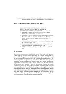
Figure 2.1: Sample structure. (a) The QDs are embedded in a field-effect structure with a semi-transparent Schottky gate deposited on top. (b) Energy band diagram of the sample structure. When above-bandgap excitation is used to excite the QD, the formation of excitonic complexes in the QD relies on the process of carrier relaxation which is random by nature. In order to deterministically control the charging state, the QDs are embedded in a n+ -Schottky structure (see Figure 2.1(a)). The Schottky gate is deposited on top of the sample and consits of 5 nm of Ti or NiCr and forms a metallic but optically semi-transparent layer. Underneath, a GaAs-capping layer is deposited followed by an Al0.4 Ga0.6 As layer that prevents the flow of electrical current through the device and impedes the holes from leaving the QD before the recombination time. The QD layer is directly situated under this blocking barrier. The QDs are charged with the electrons from the n+ -GaAs layer placed typically 25 to 35 nm below the QDs.

6

Self-assembled quantum dots

Since the QD is embedded in the Schottky structure, the position of the energy levels with respect to the Fermi level can be controlled by varying the DC electrical gate voltage. The band diagram of this structure is depicted in Figure 2.1(b).When the VB energy levels lie above the Fermi sea, the QD remains empty. An electron can tunnel from the reservoir into the QD as soon as the energy level of the lowest CB state is below the Fermi level. The Coulomb repulsion energy between two electrons is approximately 23 meV and therefore in this regime an additional electron cannot enter the QD once a single charge is present. This is the Coulomb blockade effect [15]. As a result, this structure together with the Coulomb effect allows deterministic charging of the QD with single carriers.

2.3 Spin structure Besides the motional degrees of freedom, the atomic part of the wavefunction has spin degrees of freedom. These entirely depend on the band structure of the semiconductor. For III-V semiconductors, the electrons in the conduction band are s-like states with angular momentum L = 0, whereas the holes in the valence band are p-like with L = 1. Electrons and holes are fermionic particles with spin S = 12 . ↑Z = + 1 2

↓Z = −1 2

Conduction Band

σ+

σ−

⇑Z = + 3 2

⇓Z = − 3 2

Valence Band

Figure 2.2: Pauli blockade. The four states represent the two spin states of the electron (hole) in the conduction (valence) band. The level scheme represents a negatively singly-charged QD. The right-circulary polarized component of the light is Pauli blocked due to the presence of the electron. In terms of its total angular  momentum J = L + S, the electron states can 1 , ± 1 . Similarly, three energy bands result for the hole thus be expressed as 2 2  1 , ± 1 is the split-off band (split by 100 meV due to spin-orbit interaction), states: 3 1 2 2 , ± corresponds to the light-hole band (split by some tens of meV due to strong 2 2  confinement in the QD) and 32 , ± 32 is the heavy-hole band [16]. In Figure 2.2, the four relevant states for a negatively charged QD are depicted. The optical selection rules are indicated in the absence of a magnetic field. A

2.3. Spin structure

7

1 − + ⊗ resonant laser with σ polarization creates an electron-hole pair in the state 2 e 3 + . When the excitation laser has σ + polarization, the system cannot be excited 2 h  due to the presence of an electron with spin − 12 e . This effect is referred to as Pauli blockade and results in polarization-dependent absorption due to the electron present in the QD. In the above discussion the light-hole band has been neglected due to the large splitting with the heavy-hole VB. Nevertheless, heavy-light hole mixing plays an important role in QDs. In particular, the heavy hole acquires a small contribution of the light holes and vice versa. As a consequence, the optical selection rules do not hold strictly and the diagonal transitions, originally forbiden, become weakly optically active. The oscillator strength for the diagonal transition however is suppressed by a factor of 10−3 compared to the allowed transitions thereby justifying the fact that the light-holes can be neglected to first approximation.

Experimental techniques and setup

9

3 Experimental techniques and setup In this section, the main techniques for studying single self-assembled QDs are described. In particular, photoluminescence and differential transmission are discussed. While these are standard techniques that have been used in our group for years, the direct detection of QD scattered photons is new and was developed in this thesis. This technique will be presented together with the main results on Raman photons in Chapter 5.

3.1 Photoluminescence Quantum dots can be optically investigated using micro-photoluminescence (µ − P L). Here, electron-hole pairs are optically generated in the GaAs or wetting-layer continuum in the vicinity of the QD by above-bandgap excitation. The carriers then relax on a ps timescale into the QD via carrier-phonon and carrier-carrier scattering and recombine in approximately 1 ns, emitting a photon. The different charge configurations in a QD can be studied by looking at the QD emission by varying the pump intensity of the excitation laser and monitoring the luminescence from the QD. Moreover, in our samples the number of charges in the QD is controlled by applying an electrical field to the structure as described in the previous section (see Figure 2). (a)

(b)

(c) 40 ps

1 ns

Figure 3.1: Photoluminescence spectroscopy. (a) The electron-hole pairs are created by above-bandgap excitation. (b) The carriers are captured in the QD on a ps timescale. (c) Subsequently, they recombine by emitting a photon. Figure 4 shows a typical PL spectrum as a function of gate voltage. The charging plateaus correspond to the recombination of an electron-hole pair in the presence of different number of charges. Combining µ−P L and resonant excitation spectroscopy (see section 2.2), X 1− is clearly identified as the charging plateau at higher voltages. When lowering the gate voltage, X 1− becomes unstable and its emission disappears.

10

Experimental techniques and setup

Simultaneously, the emission from X 0 becomes dominant when the Fermi level is brought below all energy levels of the CB in the QD. For further decrease of the gate voltage, the QD is positively charged with holes. At these gate voltages the electron tunnels out of the QD before recombination takes place, and due to the presence of the Al0.4 Ga0.6 As barrier, holes are trapped in the QD. The charging plateaus have a slope of approximately 0.5 µeV /mV due to the DCStark effect. The exciton has a dipole moment d~ex which responds to the electric field applied to the structure. This is observed in the emission spectrum as an energy shift which to first order depends linearly on the electric field and is given ~ by ∆EStark = −d~ex · E.

V3 V2

V1

(b) 1400

1200 V1

968

Counts/60sec

Wavelength (nm)

(a) 970

X −1

966 964 962

X0

960

X

958 0.0

0.2

+1

0.4

1000

X −1

800 600 400

0.6

0.8

1.0

958

Gate Voltage (V)

1200

Counts/60sec

Counts/60sec

V2

966

968

V3

1000

X0

800

X −1

600

958

964

Wavelength (nm)

1000

400

962

(d) 1400

(c) 1400

1200

960

X

+1

960 962 964 966 Wavelength (nm)

800

X +1 X0

600 400

968

958

960 962 964 966 Wavelength (nm)

968

Figure 3.2: Photoluminescense spectra as a function of gate voltage.(a) Photoluminescence spectra are recorded as a function of gate voltage. From (b) to (d) the individual PL spectra are shown for three different gate voltages and the charging states are indicated.

Photoluminescence allows us to identify the charging states and Coulomb interaction between the carriers. The resolution is determined by the spectrometer which in our case is approximately 30 µeV . This resolution is insufficient to investigate in detail the QD level structure because the transitions have typical linewidths of about 2 µeV . Moreover, using above-bandgap excitation many carriers are created and by Coulomb interaction alter the QD emission, leading to a line broadening.

3.2. Differential transmission

11

3.2 Differential transmission One possibility to overome the problem of limited resolution is to measure the transmission of a resonant laser field through the QD. This is done using a technique called differential transmission (DT) which is described in the following. In this case, a laser is resonant with the QD transition thereby avoiding the creation of additional carriers. The laser light interacts with the scattered light from the QD resulting in a modification of the transmitted light. The total field can be written as ET = EL + EQD where EL is the laser field represented by a Gaussian beam and EQD is the QD scattered light which can be modeled by a dipole source. The transmission is proportional to the interference of the two light field components. The total cross-section of the QD can be expressed as [17–20]: Γ2 4(w − w0 )2 + Γ2 + 2Ω2

0.0000

-0.0002

-0.0004 0

Linewidth=0.41GHz

1

2

3

Laser detuning (GHz)

4

Transmission contrast (%)

Absorption (a.u.)

σ = σ0

(3.1)

0.06 0.04 0.02 α0 = 0.05%

0.00

Isat = 14nW

1 10 100 Incident Power (nW )

1000

Figure 3.3: Absorption profile. (a) Absorption profile for a negatively charged QD. The solid line is a Lorentzian fit. (b) Saturation curve. The indicated saturation power and maximum contrast are extracted from the fit (solid line). Here, Ω is the Rabi frequency, and w the frequency of the incident laser; w0 denotes the resonance frequency of the QD and Γ is the corresponding linewidth. 2 The cross section for low powers on resonance is σ0 = 3λ , which recovers the result 2π obtained for a two-level system. The relative absorption is α = AσL , with AL the area of the laser spot. When the laser is scanned through resonance, a Lorentzian absorption profile is obtained. Figure 3.3 shows a typical absorption curve for X 1− with a linewidth of 400 M Hz, larger than the expected natural linewidth Γ0 ≈ 250 M Hz. The additional broadening has been previously observed in other groups and was attributed to spectral fluctuations [21]. The absorption as a function of laser power follows the same saturation curve as in the case of a two-level system. The saturation power is typically around 10 nW of incident laser power and is defined as the point where the absorption drops to half of its maximum value, for which the relation 2Ω2R = Γ2 is satisfied.

12

Experimental techniques and setup

The linewidth of the transition is measured by sweeping the laser accross resonance. The resolution in this case is limited by the frequency stability of the laser to around 5 − 10 MHz.

3.3 Experimental setup The spectroscopic experiments are performed using a liquid-He bath cryostat at a temperature of 4.2K. A confocal microscope set-up is mounted in an evacuated stainless steel tube that is immersed in the liquid-Helium. The tube contains He exchange gas in order to provide good thermal contact with the liquid He cooled tube walls. The cryostat is equipped with a superconducting magnet that produces fields of up to 10 T. The system is optically accessible through a top window. After travelling through the tube in free space, the light is focused through a lens of NA=0.55, which gives a resolution-limited focal spot size of approximately 1 µm2 . The sample is mounted on a stack of piezo-electric nanopositioners (Attocube ANP100/LIN) which allow the three dimensional positioning of the sample with respect to the focus. The system provides good stability, and it is possible to work with the same QD over a period of several months. (a)

(b)

Polarizer lambda-2

Sample XYZ

PBS

Figure 3.4: Experimental setup. (a) Picture of the bath cryostat top part. (b) Schematic of the experimental setup with the main components relevant for PL and DT experiments. The light transmitted through the sample is collimated through a second lens and passes through a 50/50 polarizing beam splitter cube (PBS). A pair of siliconphotodiodes (PD) collect the light from the ports of the PBS. The signal on each PD is amplified using a very sensitive, low-noise current-to-voltage amplifier with an adjustable gain (Femto OE-200-SI). In order to improve the signal to noise ratio

3.3. Experimental setup

13

(SNR), a lock-in technique is used the details of which are explained in Ref. [17–19]. Typically, a small square modulation is added to the DC part of the gate voltage with frequencies up to 3 KHz and an amplitude ranging from 40 mV to 200 mV. Due to the DC Stark effect this modulation shifts the QD in and out of resonance and thereby leads to a modulation of the PD signal. This signal is demodulated using a lock-in amplifier (Standford Research SR830 DSP). The noise is limited at low powers by the electrical noise of the preamplifier and only at powers far-above saturation shot-noise limited detection can be realized. For µ-PL spectroscopy, the sample is illuminated with a diode laser at 780 nm. The emission from the sample is collected through the fiber and sent to the spectrometer. The spectrometer has a resolution of 30 µeV . For resonant excitation we use a tunable Ti:Sa laser (MBR110, Coherent) and a tunable diode laser (Newfocus Velocity 6320). A wavemeter (High-Finesse, WSU-30) monitors the laser frequency and can lock the frequencies of both lasers simultaneously with an accuracy of better than 30 MHz. Both lasers are intensity-stabilized with an accuracy of 1 % using two sets of acoustic-optic modulators (AOMs) and a homebuilt feedback loop with PID-controllers. The AOMs can be used to pulse the lasers with typical rise times of less than 0.5 µs.

Holes in quantum dots

15

4 Holes in quantum dots The electron spin in a QD naturally defines a quantum bit and has attracted much attention in the past [4, 22]. This has not been the case for holes even though a hole is present whenever an optical excitation takes place in the QD. One of the reasons for this lack of interest is the fact that the properties of holes are much less studied and understood. For example, a complete understanding of the VB energy levels in the QD is possible only if one considers the mixing of the heavy and light-hole subbands [23]. A consequence of this mixing is the large dotto-dot variation of the hole g-factor whereas the electron g-factor is found to be homogeneous [24]. Holes have never really been thought of as long-lived quantum-information carriers due to their short spin-relaxation times in bulk III-V semiconductors, where the relaxation time is around 100 ps, several orders of magnitude shorter than that of electrons. In the case of electrons, the main spin relaxation mechanism is the spinorbit (SO) interaction which consists of two parts: the Dresselhaus SO due to the bulk inversion asymmetry and the Rashba SO due to structure inversion assymmetry [25, 26]. For holes one considers additionally the strong coupling between the heavy and light hole bands. The last mechanism explains the faster relaxation time [27]. In 2005, it was shown theoretically that in QDs the spin relaxation time for confined holes can indeed be much larger than the one for electrons due to the compressive strain and motional quantization [28]. Since then, the interest in holes has steadily increased [29–31]. In order to use the heavy-hole spin as an alternative quantum bit to the electron spin longer spin relaxation and longer decoherence time is needed. The electron spin dechorence is limited by the hyperfine interaction with the surrounding 104 − 106 nuclei [32–37]. This interaction leads to random spin fluctuations and a decoherence time of approximately 10 ns. This short time can be overcome using spin-echo techniques [38, 39] or by partly polarizing the nuclear spins [40, 41]. Unlike electrons the hole wavefunction has p-type symmetry and therefore the effective overlap with the nuclei is strongly reduced as compared to electrons [28]. Holes are therefore expected to have long decoherence times even at zero magnetic field. The predictions made for the heavy hole motivated our excursion into the physics of hole spins in QDs. Recent experiments have verified the expected long-spin relaxation time [30] and as in the case of electrons efficient spin-state preparation for the hole spin was demonstrated [29]. This chapter presents the results of the spectroscopic measurements carried out in a positively charged QD and is divided into three parts. In the first part, we present the different mechanisms used to deterministically charge the QD with a single hole. The second part deals with the polarization dependence of the absorption and discusses cooling of the hole spin. Finally, in the third part we describe two

16

Holes in quantum dots

pump-probe experiments from which we obtain values for the hole-spin relaxation time and the excited-state lifetime.

4.1. Deterministic charging of a QD with a single heavy hole

17

4.1 Deterministic charging of a QD with a single heavy hole In order to investigate a single hole in a QD it is necessary to have a deterministic control of the number of holes present. One possibility is the use of a structure with a p-doped layer as the back contact [29, 42]. In analogy to the n-doped structure, the Fermi level could then be tuned with respect to the VB energy levels in the QD and would be successively charged with the holes tunneling from the reservoir. Here we use another strategy that combines the possibility to trap single electrons and holes in the same structure. The sample investigated was already described in Chapter I: The QD-layer is situated 35 nm above the n-doped layer. The Al0.4 Ga0.6 As superlattice is deposited 12 nm above the QDs. This blocking barrier forms a triangular potential well at the interface to the capping layer which results in the quantization of the valence-band states [43, 44]. The energy of the states depends on the gate voltage applied, which defines the steepness of the confining 2D potential. The hole tunneling depends on the presence or absence of a nearby state to which it can tunnel. Due to the short distance from the QD to the blocking barrier the quantized states are all shifted out of resonance with respect to the hole state. This prohibits tunneling of the hole out of the QD. (a)

Γt

wX +1

(b)

Γt

wX 0

wX +1

Figure 4.1: Optical creation of a hole. (a) Electron-hole pairs are created using above-bandgap excitation. An exciton captured into the QD ionizes before the recombination time leaving the QD positively charged with a single hole. (b) A resonant laser creates an exciton in the QD and the electron tunnels out before recombination takes place. Resonant-excitation spectroscopy of a single hole requires a second laser that creates the hole. We achieve this in two ways: The first possibility is to create electron-

18

Holes in quantum dots

hole pairs under above-bandgap excitation as it is done for PL measurements. The second possibility is based on a resonant laser that creates an electron-hole pair in the QD. As depicted in Figure 4.1 the applied voltage is such that the Fermi level lies below the CB electron states, even when the QD is neutral. Hence, we are in a voltage regime where X0 is no longer stable. For the applied voltages the electron tunnels out of the QD with a rate Γt ≈ Γ0 to 5Γ0 [43, 44] where Γ0 is the spontaneous emission rate. When the electron tunnels out of the QD before the electron-hole recombination takes place, the QD is charged with a single hole. With this charge configuration, the laser is no longer in resonance with the transition and therefore cannot create another exciton. The situation is similar when the electronhole pairs are created non-resonantly. An exciton is captured in the QD with a rate γcap = 20−200 GHz [45]. The exciton ionizes before the recombination time, leaving the QD positively charged. In this section, the two charging methods are compared by looking at the spectral properties as well as the experimental requirements.

4.1.1 Hole charging via above-bandgap excitation In order to understand the spectral properties of a single hole it is mandatory to find the regime of stability. This refers in particular to the voltage range of the charging plateau and the pump power of the above-bandgap laser. The hole charching for this device relies on fast tunneling of the electron. The tunneling rate can be controlled by changing the voltage applied to the structure. For demonstrating this, we use DT and perform laser scan around the hole resonance for different gate voltages. The result of this plateau scan is shown in Figure 4.2. In the plot, three regimes can be distinguished. They correspond to the different chargingstate configurations of the QD. For voltages larger than V2 ≈ 0.24 V, the QD is neutral. The transition point V2 is extracted from an independent measurement of the X 0 charging plateau. In this regime, the tunneling rate is much smaller than the spontaneous emission rate Γt  Γ0 . However, when the voltage is V ≤ V2 the QD becomes positively charged with a single hole due to the fast tunneling of the electron Γt ≈ Γ0 . The rate increases when lowering the gate voltage. At V1 ≈ 0.08 V, the electron from the X 1+ excited state tunnels out with a rate Γt & Γ0 and leaves the QD charged with two holes. As a consequence, for voltages V . 0.08V the laser is no longer absorbed. From this analysis we conclude that the voltage regime with a single hole present is a stable charging configuration and lies between V1 and V2 . The reason for strong absorption in the regime of stability of X 0 is that the population of the QD depends not only on the voltage but also on the power of the above-bandgap laser. We investigate this dependence by looking at the absorptive signal of the laser resonant with the X 1+ transition as a function of the pump power. The amplitude of the absorption is a direct measure for the occupancy of the hole state. Solving the rate equations, the steady-state hole occupancy can be expressed in terms of the electron tunneling rate Γt , the hole spin relaxation rate κ, the rate Ω (proportional to the pump power P) at which the electron hole pairs are created, and Γ0 , the spontaneous emission rate of the exciton, as follows:

4.1. Deterministic charging of a QD with a single heavy hole

50

Laser Frequency Detuning(GHz)

40

X+2

X 2+

X 1+

19

X0

30 20 10 0 -10 -20 0.0

0.1

0.2

0.3

0.4

Gate Voltage(V)

Figure 4.2: DT laser-voltage scan. The absorption of the X 1+ -transition is recorded while scanning the laser frequency around the resonance for different gate voltages. The voltage regime covers three regimes of stability indicated in the figure as X 2+ , X 1+ and X 0 .

hnh i =

Γt Ω . κ Γ0 + Γt

(4.1)

Hence, the hole population reaches when the rate at which electron  its maximum Γ0 hole pairs are created is Ωsat = κ Γt + 1 , for which the occupation is hnh i = 1. The corresponding data is presented in Figure 4.3. The absorption is measured at two different voltages of the charging plateau. The pump power for which the H absorption reaches its maximum in the high voltage regime is Psat = (1.4±0.2) mW, L approximately 10 times larger than in the low voltage regime for which Psat = (0.17± 0.01) mW. The voltage dependence is consistent with the expression obtained for Ωsat . When the voltage is increased, the tunneling time of the electron Γt decreases, thereby enlarging the saturation point Ωsat . Below and above Psat two different behaviours are identified. For low powers, P ≤ Psat , the absorption increases linearly with power. In this regime the occupation of the single-hole state hnh i follows expression (4.1). Once hnh i = 1 is reached, a second hole can be captured in the QD, thereby decreasing the single hole occupancy with approximately the same rate dhnh i 1 ≈ − Ωsat hnh i. As a result, the absorptive signal decrease exponentially as a dΩ function of power in agreement with the experimental results. The measurements presented up to here demonstrate that the QD can be controllably charged with a single hole by carefully choosing gate voltage and pump power. However, above-bandgap excitation creates many electron-hole pairs in the vicinity

20

Holes in quantum dots

(b)

(a) 0.20

0.20 0.16 Absorption (%)

Absorption (%)

0.16 0.12 0.08 0.04

0.12 0.08 0.04 0.00

0.00 0

1 2 3 4 5 6 Output Laser Power (mW)

0.0 0.2 0.4 0.6 0.8 Output Laser Power (mW)

Figure 4.3: Hole occupancy as a function of pump power. The absorption of the X 1+ -transition is measured as a function of the laser pump power. The probe laser is kept constant around saturation for both values of gate voltage. Data in (a) ((b)) are taken in the high (low) voltage regime. The solid line is an exponential fit from where it is extracted a saturation power of Psat = (2.02 ± 0.08) mW (Psat = (0.16 ± 0.01) mW) in the high (low) voltage regime. of the QD. Therefore, the question arises whether the surrounding charges affect the spectral properties of the optical transition. In order to answer this question, the linewidth and the resonance position are measured as a function of pump power. The results are displayed in Figure 4.4. We observe a relatively broad linewidth with a large spectral distribution of γ = (1.5 ± 0.2) GHz. Moreover, the center frequency of the transition experiences a shift of δ ≈ 3.5 GHz. Even though the charging state of the QD remains unperturbed by the surrounding free carriers, the Coulomb interaction with the hole in the QD is significant enough to produce a shift of more than twice the linewidth. These effects are important when performing spectroscopy of the X 1+ transition with the hole being created by non-resonant excitation.

4.1.2 Hole charging via resonant excitation A second possibility for charging the QD with a single hole is resonant excitation. This kind of experiment in which the absorption of one laser, namely the laser resonantly probing the X 1+ transition, is dependent on the presence of a second laser resonant with the X 0 transition, will be referred to as conditional absorption. Absorption is only observed when pump and probe frequency exactly match the energy of the corresponding transitions for a given gate voltage. The three conditions can be found in the following way: First, a single laser is used to determine the stable charging plateau of the X 0 transition. For the lower edge of the plateau and below, the single-hole state X 1+ is the stable state. By measuring the DC-Stark shift of the X 0 transition, the frequency of the pump laser at the choosen voltage can be predicted. Once these two parameters are fixed the probe laser is scanned around

(b)

0

Linewidth (GHz)

(a)

Relative peak position (GHz)

4.1. Deterministic charging of a QD with a single heavy hole

-1 -2 -3 -4 -5

0.0

0.5

1.0

1.5

21

2.2 2.0 1.8 1.6 1.4 1.2 1.0 0.8 0.0 0.1 0.2 0.3 0.4 0.5 0.6 Output Laser Power (mW)

2.0

Output Laser Power (mW)

Figure 4.4: Resonance position and linewidth as a function of pump power. (a) Relative frequency shift of the X 1+ -transition. The solid line is a guide to the eye. (b) Linewidth of the absorption signal as a function of pump power. The dashed line indicates the average linewidth. the reference frequency extracted from the PL spectrum in order to find the X 1+ resonance.

Absorption (%)

0.08 0.00

0.08

(a)

0.00

-0.08

-0.08

-0.16

-0.16

-0.24 -0.32 0

-0.24 Linewidth=0.41GHz

1

2

3

4

Detuning (GHz)

-0.32 5

(b)

0.00

(c)

-0.04 -0.08

Linewidth=0.48GHz Linewidth=0.57GHz

-15 -12 -9 -6 -3

0

Detuning (GHz)

3

-0.12

Linewidth=0.79GHz

-6

-4

-2

0

2

4

Detuning (GHz)

Figure 4.5: DT signal for the transitions X 1− , X 0 and X 1+ . The absorption signal as a function of laser frequency detuning for (a) X 1− (b) X 0 and (c) X 1+ transition. The solid lines are Lorentzian fits with the corresponding linewidth indicated. X 1+ is broader than X 1− and X 0 by a factor of 2 and has a relatively small contrast. The X 1+ transition has a linewidth approximately twice as large as the one measured for X 1− and a reduced contrast (see Figure 4.5), the origin of which is not understood. Charging the hole by resonant excitation avoids the creation of additional charges surrounding the QD and is in this sense advantageous compared to the use of abovebandgap excitation. However, it is important to notice that this method is technically more demanding. In particular, it requires good stability of the laser frequency. When the hole is created resonantly the pump and probe lasers need to be stable better than the linewidth. Small fluctuations of one of the two laser wavelengths leads

22

Holes in quantum dots

to large fluctuations of the signal amplitude. When performing these experiments, the possibility of frequency-locking the two lasers was not available yet. However, there are several reasons that justify our inclination towards resonant scattering. The first one is based on our experimental observations which conclude that nonresonant excitation affects the spectral properties of the transition of interest. The second reason is that even though the lasers were not actively stabilized, the wavelength was constantly monitored and this allowed for correction of small drifts. The third reason is that conditional absorption presents a novel method to study this charging state that has to our knoweldge not been used before and is useful in order to measure the hole-spin lifetime.

4.2 The X 1+ transition under magnetic field Spin state preparation via spontaneous spin-flip scattering is an essential prerequisite for preparing coherent spin manipulation. For the electron spin, high-fidelity state preparation can be achieved in our sample in the presence of an external magnetic field [46]. With the aim of performing optical hole spin pumping, this section studies the response of the X 1+ transition to an applied magnetic field and the resulting polarization dependence. (a)

γ

⇑⇓↑

(b) ⇓⇑↓ Ω probe (σ − )

σ− Y

Γ

Γ

Ω probe

⇓ ⇑

πX

Ω pump

sample

λ

τ tunnel ,e

X

ξh

Ω pump (π X )

4

σ+

B σ−

0

Figure 4.6: QD level scheme in Faraday geometry and detection set-up. (a) Level scheme for X 0 and X 1+ with a magnetic field applied in Faraday geometry. (b) DT detection set-up in the circular basis. The experiments are carried out in Faraday geometry with the magnetic field pointing along the sample-growth direction. The level scheme for X 1+ in this configuration is presented in Figure 4.6. The ground states, |⇑i and |⇓i, are split by an amount gh µB B, with gh the effective hole g-factor. The holes in the excited state form a pseudo-spin singlet with spin S˜ = 0, and therefore |⇑⇓↑i and |⇑⇓↓i split according to the electron g-factor by a quantity ge µB B. The electron g-factor ge has an homogeneous distribution in the sample with a value ge = (0.56 ± 0.03). In con-

4.2. The X 1+ transition under magnetic field

23

trast, holes typically show large deviations from dot to dot, which can be attributed to the variations of In content and shape of the QD [24]. For our sample we found gh = (1.3 ± 0.2).

Normalized Absorption

1.2 1.0 0.8 0.6 0.4 0.2 0.0

0

10

20

30

40

50

60

70

Magnetic Field (mT)

Figure 4.7: Magnetic-field dependence of X 1+ absorption. Absorption of X 1+ as a function of magnetic field for circularly (•) and linearly (◦) polarized light. The two optically allowed transitions of X 1+ can be excited using σ ± circularly polarized light. In order to study the polarization dependence of these two transitions, a quarter-wave plate is introduced in the polarization sensitive detection system. One drawback of the system is the fact that the pump laser resonant with the X 0 transition also reaches the detectors, which leads to some additional noise. The detection scheme separates the two lasers completely only in case they have circular polarization and are counter-polarized. If the resonant laser probes the X 1+ transition with circularly polarized light σ − , the system is excited from the ground state |⇑i to the trion state |T↑ i = |⇑⇓↑i. The electron in the excited state sees an in-plane magnetic field component from the nuclei Bxy which leads to precession of the electron spin in 2 ns timescale [47]. The coherence of the precession is destroyed by spontaneous emission Γ into the ground state. When the system decays into |⇓i, it becomes dark due to the optical selection rules. Optical pumping occurs when the spin-flip rate of the hole ξh is smaller than the precession of the electron spin γ, the ratio of which determines its efficiency. The main processes that give rise to the spin-flip rate ξh are the spinorbit interaction and the hyperfine interaction with the nuclei. At zero magnetic field spin-flips involving a single phonon are absent. Moreoever, hyperfine interaction is expected to be smaller because the hole wavefunction has p-symmetry [28]. As a consequence, the system would remain dark for as long as the hole lifetime. The situation is different for electrons for which an external magnetic field is required in order to observe spin-pumping. The hyperfine interaction with the nuclei prevents the preparation of the electron spin at 0 T and is also the main decoherence source.

24

Holes in quantum dots

A way to experimentally confirm optical pumping at 0 T is to compare the absorption of the resonant laser for both circular and linear polarization. While we expect spin-pumping for circularly polarized light, for linearly polarized light the system never falls into a dark state and spin pumping is avoided. In Figure 4.7, the results of the measurement are presented. Unexpectedly, we observe no spinpumping at zero magnetic field independent of the polarization. Significant cooling and a dependence on the polarization is only observed for finite magnetic field.

4.2.1 Influence of the light ellipticity on the optical spin pumping One possible explanation for the absence of cooling at zero magnetic field is that our laser is not perfectly polarized. Whereas for X 1− spin cooling is observed at a finite magnetic field, for X 1+ we expect cooling at zero magnetic field. The fact that the two transitions are energetically degenerate could lead to a strong sensitivity of the absorption to small imperfections in the polarization. A theoretical study based on the rate equations is presented in order to clarify the effect of ellipticity.

ξh γ ξh γ ξh γ ξh γ

1.0

Cooling

0.8 0.6

=0 = 0.09 = 0.23 = 0.53

0.4 0.2 0.0 0.0

0.2

0.4

ε

0.6

0.8

1.0

Figure 4.8: Cooling efficiency as a function of light ellipticity. Theoretical expectation for the amount of spin cooling as a function of the light ellipticity , for different spin-flip ratios ξγh .

First, we find an expression for the amount of cooling for a laser probing only one transition. The dependence of the cooling on the different physical parameters can be found by solving the rate equations for the four-level system depicted in Figure 4.6. The rate equations can be written as:

4.2. The X 1+ transition under magnetic field

dN⇑ dt dN⇓ dt dNT↑ dt dNT↓ dt

25

= −ΩN⇑ − ξh (N⇑ − N⇓ ) + ΓNT↑

(4.2)

= ξh (N⇑ − N⇓ ) + ΓNT↓

(4.3)

= ΩN⇑ − ΓNT↑ + γ(NT↑ − NT↓ )

(4.4)

= −γ(NT↑ − NT↓ ) − ΓNT↓

(4.5) (4.6)

where N⇑(⇓) represents the population of |⇑ (⇓)i state and NT↑(↓) accounts for the  population of the excited states T↑(↓) = |⇓⇑, ↑ (↓)i. The amount of cooling ΞC is expressed in terms of the steady-state ground state populations ΞC =

N⇓ − N⇑ = N⇓ + N⇑ 1+

1 . 2ξh (Γ + 2γ) γΩ

(4.7)

The cooling is maximum (ΞC = 1), when all the population is in the state |⇓i. In the case of thermal equilibrium, the population of the two ground states is the same N⇑ ≈ N⇓ and no cooling is observed (Ξ = 0). The expression reflects the qualitative description given above. In particular, the amount of cooling decreases for larger ξh because spin-flips randomize the ground state population leading to thermal equilibrium. Additionally, the amount of cooling increases for larger values of γ. Indeed if γ = 0, the decay to |⇓i would not be possible. Imperfections in the polarization are described by introducing an additional σ + Ω(σ + ) polarization component with an amount  = Ω(σ − ) . The amount of cooling as a function of  is now expressed according to Ξ=

1− . h 1 +  + 2ξ (Γ + 2γ) γΩ

(4.8)

In Figure 4.8, Ξ is plotted as a function of  going from circular polarization  = 0 to linear polarization  = 1 and for different values of hole and electron spin-flip ratio ξγh . The polarization achieved experimentally lies in a range between 80% and 95% ( = 0.05−0.2) for which the theory predicts optical spin pumping to be observable. As a conclusion, imperfections in the polarization should not be responsible for the complete suppression of cooling. As discussed earlier the thermalization of the hole spin and consequently the absence of spin cooling could also be due to a short hole lifetime. For this reason, we have performed lifetime measurements of the ground and excited states of the X 1+ transition which will be presented in the next section. In the presence of a magnetic field, the absorption of the circularly polarized light is significantly reduced. From the data in Figure 4.7, we observe a reduction of 72% at a magnetic field of 60 mT as compared to the absorption at zero magnetic field.

26

Holes in quantum dots

This indicates a magnetic field depence of the spin flip rates γ or ξh . We performed optical pumping experiments in the same structure for the electron spin. There we found that the electron spin-flip rate is strongly supressed even under relatively weak magnetic fields [46], thereby reducing the spin-flip rate γ. As seen before, a reduction in γ directly decreases cooling. However, we observe that the cooling is increasing, from which our simple model concludes that ξh decreases more strongly with magnetic field than γ. This again is contradictory to our expectation that ξh is independent of magnetic field because of the negligible hyperfine interaction with the nuclei. This was recently confirmed by Warburton et al. [29] where they efficiently spin pumped the hole spin. A further possible explanation would be a strong dependence of the hole-spin relaxation time on the magnetic field.

4.3 Hole spin relaxation time (T1) and trion lifetime measurement In this section we present the results of a pump-probe experiment which gives a lower bound for the hole spin relaxation time of T1h ≥ 20µs. In addition, we study the stability of the excited state. Both measurements are aimed at clarifying the absence of spin cooling at zero magnetic field.

(a)

Absorption Ratio r{ X1+X0}

T 1+

(b)

6

~ Γt

5 4

X0

3 2 1 0

Ω pump

Γ0 0.10 0.12 0.14 0.16 0.18 0.20 Gate Voltage (V)

Γ1+

Ω probe

Γt h

κ

0

Figure 4.9: Absorption ratio of probe vs. pump laser as a function of gate voltage. (a) Absorption ratio rX 1+ X 0 of the probe laser at the X 1+ -transition vs. the pump laser at X 0 for different values of the gate voltage. (b) Level scheme for X 0 and X 1+ and the mainly contributing decay rates. The instability of the X 1+ transition is first studied by looking at the absorption ratio of probe vs pump laser both in CW mode. In a regime where X 1+ is longlived, the pump is only meant to create the hole in the first place, and consequently absorption from the pump should be small. Figure 4.9 displays the measured absorption ratio as a function of gate voltage. Significant absorption is observed for

4.3. Hole spin relaxation time (T1 ) and trion lifetime measurement

27

the pump laser, indicating that the transition is stable on a relatively short time scale. When we tune to lower gate voltages X 1+ becomes more stable and the probe absorption increases relative to the pump. The instability of the transition is either due to the ground or the excited state being unstable. When the system is in the trion state an electron (hole) could tunnel in (out), form a biexciton XX (X 0 ) and subsequently decay into the neutral X 0 state. This process with rate Γ˜t is indicated in Figure 4.9(b). Solving the rate equations for the system, the absorption ratio rX 1+ X 0 can be expressed in terms of Γ˜t , the electron tunneling time Γt and the hole-spin relaxation rate κ as follows rX 1+ X 0

Ωpump Γt = Ωprobe

(

˜t Γ0 Γ (Γ0 + Γt ) + Ωprobe Γ1+ + Γ˜t κ

)−1 .

(4.9)

The natural linewidth of X 1+ is Γ1+ ≈ Γ0 . We assume Γt ≈ Γ0 . With these considerations we can extract an approximate value for κ and Γ˜t in the two following regimes: In case that the spin-hole relaxation rate dominates over the excitated state lifetime κ  Γ˜t we obtain a value of κ ≈ 0.03 GHz. In the opposite regime the dominant process is the relaxation from the excited state κ  Γ˜t and we obtain Γ˜t ≈ 0.12 GHz. Whether we lie in one of these two regimes or the rates are similar to each other κ ≈ Γ˜t is distinguished in the following pulsed experiments.

τ on 5 µs

(b) τ off

ON OFF

ON

pump

probe

Absorption (%)

(a)

0.15 0.10 0.05

OFF

0.00

0

2

4

6

τ off ( µ s )

8

10

Figure 4.10: Probe absorption as a function of pulse delay. (a) Using an AOM, the pump laser is pulsed for a duration of τon = 5 µs with a variable time delay between subsequent pulses, τof f . The probe laser is on continuously. (b) Probe absorption as a function of τof f . In the first experiment, the pump laser is pulsed with an AOM which gives pulses with a rise and fall time of less than 0.5 µs. The pulse duration of the pump τon is fixed to 5 µs. The time between pulses (τof f ) varies from 0 to 10 µs. The laser resonant with the X 1+ transition is present all the time. The results in Figure 4.10 demonstrate a decrease in absorption α as a function of the delay time between two consecutive pulses.

28

Holes in quantum dots

The decrase can be theoretically modelled assuming an exponential decay for the lifetime of the ground or excited state. Note, that this experiment does not yet distinguish between the ground or excited-state lifetime. Here, we consider a decay rate γ˜ , which entails both the ground and excited state lifetime. The absorption can then be expressed as   1 τon −˜ γ τon −˜ γ τof f ) . (4.10) + e (1 − e α = α0 τon + τof f γ˜ (τon + τof f ) Here α0 is the absorption for zero time delay, i.e. continuous excitation of the X transition. The first term in the formula corresponds to the reduced absorption during the time duration of the pump. The second term describes the absorption after switching off the pump. With this expression we obtain a decay time τ = (5.9 ± 0.9) µs, which corresponds to a rate γ˜ ≈ 0.17 MHz. We perform a second experiment that directly measures the hole-spin relaxation time. In this experiment, a sequence of two pulses is used in order to measure the hole lifetime independently from the excited-state lifetime. Both pump and probe lasers are now pulsed. The duration and frequency of the pulses are kept constant, while the delay time between pump and probe is varied. As a consequence, the absorption signal remains constant as long as the delay time between pulses is much shorter than the spin relaxation time of the hole. A delay time greater than T1h would show up as a reduction of the signal. The result of the experiment is presented in Figure 4.11 and confirms that the hole remains in the QD for a time as long as 20 µs. For the different delay times the absorption shows no decrease at all and therefore the hole spin relaxation must be significantly longer than T1h ≥ 20 µs. 0

(b) 0.20

(a)

0.16 pump

OFF 24 µs

2 µs

ON

probe OFF

τ Delay

Absorption (%)

1 µs ON

0.12 0.08 0.04 0.00

0

3

6

9

τ Delay

12

15

18

Figure 4.11: Pulsing pump and probe. (a) The pump and probe lasers are pulsed using two AOMs controlled via a delay pulse generator (DG 535) which varies the delay time τDelay between the pulses. (b) Probe absorption as a function of the delay time between pump and probe. Hence we see that while the hole state itself is long-lived, the excited state lifetime is reltively short. However, this short lifetime effectively increases the spin-flip rate

4.3. Hole spin relaxation time (T1 ) and trion lifetime measurement

29

of the excited state γ and therefore has the effect of increasing (and not decreasing) the efficiency of spin-pumping. Consequently, given the lifetime measurements, it is still an open question why we could not observe spin cooling at zero magnetic field.

30

Holes in quantum dots

4.4 Conclusion In summary, the measurements presented helped us to understand the behaviour of a QD charged with a single heavy hole. Deterministic charging of a single hole was achieved by using a field effect structure with an electron reservoir. This structure allows one to investigate both single electrons and holes by varying the applied gate voltage. Hole charging relies on fast tunneling of the electron Γt and the presence of the blocking barrier placed above the QDs. The tunneling rate Γt was shown to be voltage dependent and therefore it was possible to controllably define a stable regime for a single hole in the QD. Using above-bandgap excitation, the hole occupancy was controlled by varying the pump power. However non-resonant excitation creates additional charges surrounding the QD that affect the spectral properties of the X 1+ transition. In particular, these extra charges caused large spectral fluctuations which manifested themselves in a large linewidth as well as a shift in the transition energy when increasing the pump power. In order to avoid these effects, we have used resonant excitation to create the hole. Conditional absorption is a novel technique that allowed us to measure the hole lifetime in a pulsed pump-probe experiment. We obtained a hole lifetime of T1h ≥ 20 µs and an excited state lifetime of T1exc = (5.9 ± 0.9) µs. The long spin relaxation times for the hole is very promising. However, the lifetime measurements do not explain the absence of spin cooling at zero magnetic field. The fact that there is no cooling indicates the presence of a spin-flip mechanism the origin of which could not be revealed. Further analysis on holes could be done in other types of structures, for example in p-doped structures for which spin cooling has been observed [29]. In particular, it would be interesting to investigate the origin of the different behaviour of the two structures.

Negatively charged quantum dots in Voigt geometry

31

5 Negatively charged quantum dots in Voigt geometry In 1991, the phenomenon of Electromagnetically Induced Transparency (EIT) was observed for the first time using atomic strontium vapour [48]. Since then, it has observed in many different settings, varying from ultracold matter to solid-state systems. EIT denotes an interference effect through which a light-absorbing medium becomes transparent by applying a second light field. The transparency experiment is usually realized in a λ-system and its observability depends strongly on the dephasing of the two ground states involved, γ21 [49]. Performing EIT for a single electron or hole in a QD provides information on the decoherence time. Repeating EIT experiments for different parameters, for example at different gate voltages and a fixed magnetic field would allow to determine the contribution of co-tunneling processes to γ21 . Conversely, setting the gate voltage at the center of the absorption plateau where co-tunneling is minimal and changing the magnetic field allows for the determination of the contributions from hyperfine interactions and from phonon mediated processes by exploiting their specific magnetic field dependences. In contrast, co-tunneling is expected to be magnetic-field independent in the regime where optical wave-functions are not modified appreciably and one could verify this by varying the magnetic field at the edge of the plateau, where γ21 is determined by co-tunneling. Additionally, EIT allows for the preparation of any arbitrary quantum state by stimulated Raman adiabatic passage [50]. A first step for realizing EIT is the ability to perform high-fidelity state preparation of the electron or hole spin. In our sample this has been realized successfully for electrons and therefore this chapter focuses on negatively charged QDs. The first section of the chapter reviews the basic principles of EIT and dicusses the feasibility of using this interference effect as a means to study the decoherence of the electron spin. The second part analyzes the advantages of defining a λsystem in Voigt as compared to Faraday geometry. In the third part, we present experimental results in the Autler-Townes as well as the EIT regime. Finally, the fourth part discusses the influence of the hyperfine interaction with the nuclei on the EIT profile.

32

Negatively charged quantum dots in Voigt geometry

5.1 EIT - a tool for studying decoherence EIT is typically performed in a three-level system using two monochromatic light fields. There are three types of suitable three-level systems - the Lambda, Ladder and Vee configurations [49]. Here we focus on the λ-system, which offers the widest range of applications and is straightforward to realize in a QD. The system (depicted in Figure 5.1 (a)) consists of two dipole-allowed transitions, |1i − |3i and |2i − |3i, which are both coupled by electromagnetic fields usually referred to as probe and coupling laser. The transition from |1i to |2i is optically forbidden and the two ground states are metastable.

∆2

∆1 ΩC

Γ31

Γ32

ΩP

1

2

(b)

3

Absorption (a.u.)

(a)

Ω C ≥ γ 31 Ω C ≤ γ 31

1.5

1

0.5

γ 21

2

0

-4

-2

0

∆ 1 / γ 31

2

4

Figure 5.1: EIT in a λ-system.(a) λ-system with the main mechanisms of spontaneous emission and dephasing rates indicated. (b) Theoretical expectation of the absorption profile in the Autler-Townes regime (Ωc ≥ γ31 ) and the EIT regime (Ωc ≤ γ31 ) with γ21 = 0 and ∆2 = 0. In the absence of a coupling laser, Ωc = 0, the probe laser absorption shows a typical Lorentzian lineshape as a function of frequency detuning. The response of the system is modified in the presence of the coupling field. Using a master-equation formalism one can express the linear susceptibility as [49]: 2 4δ(|Ωc |2 − 4δ∆1 ) − 4∆1 γ21 |µ13 |2 ρ χ (−wp , wp ) = 0 ~ |Ωc |2 + (γ31 + i2∆1 )(γ21 + i2δ) 2 (1)

|µ13 |2 ρ 8δ 2 γ31 + 2γ21 (|Ωc |2 + γ21 γ31 ) +i 0 ~ |Ωc |2 + (γ31 + i2∆1 )(γ21 + i2δ) 2 Here ∆1 and ∆2 are the one-photon detunings for the two light fields, as depicted in Figure 5.1, δ = ∆1 − ∆2 is the relative or two-photon detuning, and Ωc denotes the Rabi frequency of the coupling laser. The total spontaneous emission rate is Γ3 = Γ31 +Γ32 . Let the rates γ3deph and γ2deph describe the main dephasing processes of levels |2i and |3i, the rates γ31 and γ32 are defined as γ31 = γ3deph + Γ3 , γ32 = γ3deph + γ2deph + Γ3 .

5.1. EIT - a tool for studying decoherence

33

The absorption of the probe laser is given by the imaginary part of the susceptibility. Its profile is depicted in Figure 5.1 (b) for γ21 = 0. Two distinct situations can be differentiated: the Autler-Townes (AT) and the EIT regime. In the AT regime, the Rabi frequency of the coupling laser is larger than γ31 , Ωc ≥ γ31 , and the absorption profile consists of approximately two Lorentzians split by Ωc . AT splittings have previously been observed in QDs [51–53]. EIT occurs for small values of the Rabi frequency Ωc ≤ γ31 . In this case, the original 2 Lorentzian shows a narrow transmission window with a linewidth γΩ31c  γ31 . In both Autler-Townes and EIT regime, the cancellation of the absorption for zero detuning, δ = 0, makes the medium transparent to the probe laser. This cancellation can be understood as the destructive interference between the two following optical excitation paths. The first one is a direct excitation from |1i to |3i and the second path is an indirect excitation |1i- |3i - |2i - |3i. The amplitude of the indirect path has the same magnitude as the direct path due to the strong coupling laser but with opposite sign leading to a destructive interference. This interference affects both the absorption of the transmitted laser as well as the state of the system. The system is in a dark state, a superposition of the two ground states from which no absorption or emission can take place. In practice, the dephasing rate is non-zero γ21 6= 0 and the transparency is no longer perfect. Instead, when the probe and the coupling lasers are resonant with the transition (δ = 0, ∆1,2 = 0) the absorption χ00 takes the form χ00 ≈

Ω2

2γ21 . + γ21 γ31

(5.1)

In this case, EIT and Autler-Townes are still observable if γ21 is smaller than 2 the width of the transmission window, i.e. γ21  γΩ31c . This in turn imposes a condition upon the Rabi frequency of the coupling laser: varying the laser intensity one goes from the EIT regime where Ω2c  γ31 γ21 to a regime where EIT is no longer visible Ω2c  γ31 γ21 . In this way, one can extract valuable information on the spin-decoherence time of the electron or hole spin states, provided we know the spontaneous emission rate of the excited state and the Rabi frequency of the laser. The spontaneous emission can be determined using time-correlated single-photon counting experiments [54] and the Rabi frequency is estimated from a measured saturation curve.

5.1.1 Frequency stabilization As previously mentioned, maximum transparency of the medium occurs when the two-photon detuning condition is fulfilled, i.e. δ = 0. Fluctuations in δ can washout the EIT signal and it is therefore important to frequency-stabilize the probe and coupling lasers. The two lasers are locked onto a wavemeter usign a software lock, which ensures a stability of typically 5 to 10 MHz. Alternatively, the relative frequency between the probe and coupling laser ν1 − ν2 was stabilized using the optical phase-lock depicted in Figure 5.2. The two laser fields are combined on a fast photodiode which generates a beat signal on the microwave regime. Subsequently, the signal is

34

Negatively charged quantum dots in Voigt geometry

VCO

TiSa laser

ν1 ν2

3 - 8 GHz Voltage-controlled oscillator

ν1-ν2 Photodiode BW >5GHz

power splitter 1/2 Mixer loop filter directly to diode

fast

PID slow

Velocity laser current control

Figure 5.2: Setup of phase-lock. Schematics of the phase-lock loop used to stabilize the frequency difference between probe and coupling lasers. amplified by 20 dBm and mixed (down) with the synthesized signal from a voltagecontrolled oscillator (VOC, Gigatronics 910). The VCO generates microwaves in a frequency range between 3 and 8 GHz. The resulting signal is divided into two parts of equal power. One of them is sent to a PID lock-box and subsequently to the current control of the laser controller. This part corrects for slow drifts of the laser frequency. The other component is sent through a loop filter directly to the current modulation input of the diode laser and compensates for fast fluctuations of the laser. The measured width of the beat signal between the two lasers was less than 100 KHz-sufficient for the purpose of this experiment.

5.2 λ-system in Voigt geometry For the X 1− -transition, a λ-system can be defined with the two spin states of the electron |↑i and |↓i and one of the excited trion states. At zero magnetic field the two excited states are degenerate. Therefore, isolating a three-level system requires the presence of a magnetic field such that the induced Zeeman splitting is larger than the natural linewidth. The first requirement to form a λ-system is that the upper level should be optically accessible from both ground states. In Faraday geometry, this is possible due to heavy-light hole mixing that makes the transition |↓i-|↑↓, ⇑i optically weakly allowed. However, photon absorption and emission are suppressed by a factor of approximately 10−3 with respect to the optically fully allowed transition |↑i-|↑↓, ⇑i. As a consequence, the laser intensity of the weak transition needs to be relatively strong and large detunings are required in order for the absorption on the other transition to be negligible. In addition, the two lasers have the same circular polarization and are indistinguishable in our polarization sensitive detection set-up, which leads to additional noise in the detectors.

5.2. λ-system in Voigt geometry

(b)

↑↓⇑

313560

X

↑↓⇓

πY

πX

Γ 2

ΩC

Γ 2

Ω Pr obe

↓ ↑

X

X

X

γ spin

Laser frequency (GHz)

(a)

35

313555 313550 313545 313540 313535 0.50

0.52

0.54 0.56 0.58 Gate Voltage(V)

0.60

0.62

Figure 5.3: Voigt geometry. (a) Level scheme of X 1− in a magnetic field in Voigt geometry. Probe and coupling lasers couple the relevant transitions of the λ-system. (b) Absorption is measured as a function of laser frequency and gate voltage at a magnetic field of B = 0.6 T. Spin cooling is observed away from the plateau edges. The absorption is recovered in the middle of the plateau around VG ≈ 0.57 V where a second laser with opposite polarization repumps the electron spin. A more suitable system is obtained in Voigt geometry [55] (see Figure 5.3). The spin states expressed in terms of the Faraday-basis are: |↑ix = √12 (|↑i + |↓i) and |↑ix = √12 (|↑i − |↓i). Voigt geometry has the advantage that the four transitions are optically allowed and have the same strength. Moreover the two transitions forming a λ-system have linear and opposite polarizations which is technically favourable for suppressing the coupling laser on the detector. In Voigt geometry, spin cooling is more efficient than in Faraday geometry since the excited state decays via spontaneous emission to the two ground states with equal probability. This ensures the population to be in the |↓ix state when the coupling laser is stronger than the probe laser. Another requirement for performing EIT is that the dephasing rates should satisfy the two requirements: Ω2c ≥ γ31 γ21 and Ωc ≤ γ31 . In our case γ31 ≈ Γ0 and therefore the ground state dephasing rate must be smaller than the natural linewidth γ21 ≤ Γ0 . Consequently, the best EIT regime should be found by avoiding or minimizing the two main mechanisms of dephasing, i.e. co-tunneling and hyperfine interaction with the nuclei. Co-tunneling due to the interaction with the electron reservoir is supressed in the middle of the plateau due to the relatively large tunneling barrier in our sample of 35 nm. Hence, the best working regime is the regime of spin cooling.

5.2.1 In-plane hole g-factor The in-plane hole g-factor gxy has been predicted in several theoretical studies to be negligible [56]. In our sample, we find a large inhomogeneity similar to the one found for the hole g-factor in the growth direction. Recent experimental studies saw

36

Negatively charged quantum dots in Voigt geometry

a direct correlation between the g-factor and the XY splitting of the X 0 -transition and concluded that the inhomogeneity is related to the in-plane asymmetry of the QD shape [57]. Absorption spectra for three different types of QDs with different hole g-factors are shown in Figure 5.4. The first one has a g-factor gh ≈ 0. In this case, a single λ-system cannot be well isolated because the two excited states are degenerate. In the second case, the magnitude of the g-factor is the same for both the electron and hole gh ≈ −ge . We found this configuration in 2 out of 15 dots. Here, the two inner transitions are degenerate. Hence a laser couples both transitions at the same time. In the measurements, we mainly used QDs with different electron and hole g-factors gh 6= ge . For high-enough magnetic fields the influence of the fourth level is negligible in this case.

Absorption (%)

0.02

(a)

(c)

(b)

0.00 -0.02 -0.04 -10

-5

0

5

10

Laser detuning (GHz)

-9

-6

-3

0

Laser detuning (GHz)

3

-5

0

5

10

15

Laser detuning (GHz)

Figure 5.4: In plane hole g-factor. Absorption profile as a function of detuning for three different QDs at a magnetic field of 0.6 T. The hole g-factors are: (a) gh ≈ 0 (b) gh ≈ −ge and (c) gh 6= ge .

5.2.2 Technical requirements In order to apply a magnetic field in Voigt geometry two new sample holders were desgined. The first one (see Figure 5.5(a)) consists of a total of six permanent magnets placed at a distance of 0.5 mm from the sample. This configuration gives a homogeneous field within the gate area of the sample with maximum fields of 0.6 T. With the second holder (Figure 5.5(b)), the sample and the corresponding optical elements are tilted by 90◦ . This make it possible to use the superconducting magnet and to apply magnetic fields up to 10 T.

5.3 Autler-Townes splitting and EIT regime First, we present the results for a QD with an inner splitting of 2.5 GHz and an outer splitting of 5 GHz at 0.6 T. The experiment was carried out using the holder with the permanent magnets. For low magnetic fields, the inner and outer splittings can be expressed as ∆Ein ≈ (ge − gh )µB B and ∆Eout ≈ (ge + gh )µB B, from which we obtain an electron g-factor ge ≈ 0.45 and a hole g-factor gh ≈ 0.15.

5.4. Influence of hyperfine interaction on the EIT profile

(a)

37

(b) lens PBS

Permanentmagnets

sample

Photodetector

Figure 5.5: Sample holders for applying a magnetic field in Voigt configuration. (a) Sample holder using six permanent magnets. The sample is placed between them and the detection setup is placed below the sample. (b) Sample holder which enables the use of the superconducting magnet. The sample is located on top of the nanopositioners, which allows independent 3D positioning with respect to the holder.

The measurement is performed in the middle of the plateau where spin pumping takes place due to the strong coupling laser. The probe laser has orthogonal polarization. In order to avoid fluctuations that could smear out the absorption profile, the laser power was stabilized to less than 1%. From the saturation curve, the saturation power is determined to Psat = 28 nW. The probe power is stabilized below saturation at P ≈ 0.3Psat . The absorption signal of the probe laser was recorded for different pump powers ranging from the Autler-Townes regime to the EIT regime. Figure 5.6 shows four scans in the Autler-Townes regime. The results obtained follow the theoretical prediction (see Figure 5.7). The splitting corresponds to the Rabi frequency Ωc when we consider γ31 ≈ Γ0 and a natural linewidth of Γ0 ≈ 0.2 GHz, close to the typical values in our QDs [46]. When decreasing the power down to Ωc = 1.6 Γ0 the absorption is a single peak without additional structures. This is a general trend observed for all the QDs investigated in this sample: the two peaks close up before the EIT regime is reached. This unexpected result could be due to fluctuations on the two-photon detuning. The physical origin of these fluctuations is the subject of investigation in the next section.

5.4 Influence of hyperfine interaction on the EIT profile Most QDs exhibit fluctuations on the absorption amplitude even for fixed external parameters. In Figure 5.8 the absorption of X 1− is measured as a function of time for a fixed gate voltage and a laser frequency locked with an accuracy of 10 MHz.

38

Negatively charged quantum dots in Voigt geometry Ω C = 3.3 γ 31

(b) normalized signal

1.2 0.8 0.4 0.0

3.2 4.0 4.8 5.6 Frequency detuning (GHz)

(d)

normalized signal

(c) 1.2 0.8 0.4 0.0

3.2 4.0 4.8 5.6 Frequency detuning (GHz)

normalized signal

normalized signal

(a)

1.2 0.8 0.4 0.0

3.2

4.0

4.8

5.6

Frequency detuning (GHz)

1.6 1.2 0.8 0.4 0.0 3.2 4.0 4.8 5.6 Frequency detuning (GHz)

Figure 5.6: Autler-Townes split QD lines. Absorption profile measured for a QD at a magnetic field of B=0.6 T in the Autler-Townes regime for different Rabi frequencies of the coupling laser: (a) Ωc = 2.3 γ31 , (b) Ωc = 3.3 γ31 , (c) Ωc = 4.6 γ31 and (d) Ωc = 8.5 γ31 . Outside the QD resonance the noise is relatively low compared to the large onresonance fluctuations. The origin of the fluctuations can be twofold. On the one hand, we expect variations of the charge enviroment to move the QD energy levels. The shift is equal for all levels with the same charging state. This corresponds to an increase or decrease of the one-photon detuning. This should not affect the two-photon detuning condition for which a cancellation of the absorption should be observed regardless of the position of the upper level. However, the bandwidth of the EIT will decrease. The EIT profile is most affected by spin-dependent fluctuations due to changes in the magnetic enviroment. Here, we mainly discuss the influence of the nuclei due to hyperfine interaction with the electron. Besides the external magnetic field, the electron experiences an effective magnetic field (Overhauser field) due to the hyperfine interaction with the nuclei [58]. If the nuclei are not polarized, the effective field fluctuates with a mean ∆Bnuc ≈ 15 mT. Our experiments are typically carried out at magnetic fields Bext  ∆Bnuc , where the spin flips are energetically forbidden due to the large Zeeman splitting. A requirement for the experiment to be successful is that the Overhauser field should not change on the timescale of the experiment (approximately 1 sec). Random nuclear-spin induced magnetic-field fluctuations change the splitting between

Autler-Townes splitting (GHz)

5.4. Influence of hyperfine interaction on the EIT profile

39

1.5 1.2 0.9 0.6 0.3 0.0 0

30

60

90

120

150

P/Psat

Figure 5.7: Autler-Townes splitting. Magnitude of the Autler-Townes splitting extracted from the measured absorption profile as a function of coupling-laser power. The solid line is a fit based on the theoretical expectation. (b)

(a)

Absorption (%)

0.00 -0.03

A A

-0.06

B

-0.09 B

-0.12 0.50

0.51 0.52 Gate voltage (V)

0

30

60

90

120 150

Sampling points

Figure 5.8: Noise measurement on X 1− . (a) DT as a function of gate voltage. (b) DT as a function of time for fixed external conditions. The laser frequency and laser intensity are stabilized. Each data point is averaged over 100 ms. the two ground states. Consequently the two-photon detuning condition for which EIT is observable would also fluctuate and the experiment would reveal a very short coherence time or even no EIT would be observable if the fluctuations are too fast. Narrowing the fluctuations of this component would ensure that the measured coherence time is only limited by the actual decoherence. Recent experiments in the group have shown that there is a regime for which an optically probed QD resonance is locked via a feedback mechanism mediated by dynamic nuclear spin polarization (DNSP) [59]. When the laser is detuned from its resonance value, the nuclei polarization changes accordingly and thereby shifts the electron ground state such that the laser is kept on resonance and maximum absorption is achieved. This process happens on a time scale on the order of seconds and therefore it is observed only when the laser is scanned slowly through the resonance. Whenever the laser frequency is changed, DNSP ensures that the energy transition

40

Negatively charged quantum dots in Voigt geometry

Absorption (%)

is always kept on resonance thereby producing a dragging effect. The extend of the dragging depends on the decay timescale of the nuclear spin polarization. For an empty QD, the nuclear spin polarization decays on timescales exceeding an hour. The decay times are significantly reduced in the presence of an electron and depend mainly on the tunneling time as well as the external magnetic field [60]. Experiments done in a 25 nm tunneling barrier sample yielded decay times up to 4 sec at a magnetic field of 4.5 T. The decay time increases when the interaction with the electron reservoir is reduced. In particular, our sample has a 35 nm tunneling barrier and therefore we expect larger decay times. However our experiments were typically performed in a magnetic field range of 0.6 T to 2 T, lower than the 4.5 T [59]. Accordingly, coherent population trapping has recently been observed for a negatively charged QD in a sample with a tunneling barrier of 80 nm at a magnetic field of 2.64 T [61]. 0.00

(a)

(c)

(b)

-0.04 -0.08 -0.12 -4

-2 0 2 4 Laser detuning (GHz)

-4

-2 0 2 4 Laser detuning (GHz)

-4

-2 0 2 4 Laser detuning (GHz)

Figure 5.9: Dragging. Absorption at B=2.5 T with the laser scanned (a) backwards and (b) forwards. (c) Pump and probe lasers are blocked between each point for approximately 1 to 3 sec. Each data point is averaged over 3 sec. The origin of dragging is not yet fully understood. Intuitively one might suspect that EIT would be better observable in a regime where dragging is predominant and the Overhauser-field fluctuations are slow. However, dragging seems to be mainly induced by the excitation laser [59] and it is therefore not clear how dragging modifies EIT in the presence of the two lasers in the two-photon detuning condition. Our experimental results seem to indicate that dragging obscures the observation of small splittings already in the Autler-Townes regime. This effect varies from dot to dot due to the different nuclear enviroment. Figure 5.9 shows the absorption measured as a function of the probe laser for a QD subject to a magnetic field of 2.5 T. The power regime is such that one expects an Autler-Townes splitting of 1.6 GHz. The absorption profile is strongly dependent on the laser scan direction, which resembles the dragging experiments. In order to eliminate this effect, the pump and probe laser were blocked between each data point for approximately 1 to 3 sec. As a result we obtained an absorption curve which was no longer dependent on the scan direction. However the curve does still not correspond to the expected two lorentzians but it shows maximum absorption over 2 GHz.

5.5. Conclusion

41

5.5 Conclusion In this chapter, the X 1− -transition has been studied under the presence of a magnetic field in Voigt geometry. In particular, the effect of EIT requires high-fidelity preparation which was successively performed. In order to define a λ-system, Voigt geometry was shown to be more suitable than the usual Faraday geometry. The optical selection rules determine the polarization of both the vertical and diagonal transitions to be orthogonal to each other. Experimentally this allows for efficient polarization separation of the coupling and probe lasers. The recombination from the excited state takes place on a nanosecond timescale with equal probability for decay into each ground state. This is in contrast to Faraday geometry, where this branching ratio is typically on the order of 10−3 . The Autler-Townes splitting followed the theoretical prediction as a function of the coupling power. However, for lower powers the splitting was no longer observable. Similary, the transmission window expected in the EIT regime could not been observed yet. The lineshape obtained instead was very much dependent on the QD studied. In most of the QDs investigated the phenomenon of dragging results in absorption lineshapes that are difficult to interpret, both in the Autler-Townes and EIT regimes. A better understanding of this effect is needed in order to estimate its influence on the EIT absorption profile and to find a suitable working regime.

A tunable Raman-scattered photon source

43

6 A tunable Raman-scattered photon source This Chapter is based on publication [62]. In order to probabilistically entangle two QDs that are energetically close to each other an independent knob to ensure spectral overlap of the emitted photons is needed [63]. In this Chapter, we demonstrate such a knob. We report on the first direct observation of all-optically tunable spontaneous Raman fluorescence from a single self-assembled QD. We demonstrate the frequency tunability of the Raman photons with magnetic field. While magnetic fields could in principle be used to tune two emitters in resonance with each other, all-optical manipulation is more versatile, faster and allows spatial addressing of several QDs within one sample. For this reason, in a second experiment the magnetic field is fixed and we vary the excitation-laser frequency to optically tune the frequency of the emitted photons over a range of roughly 2.5 GHz. From the raw data, we extract the number of scattered photons, their center frequency and linewidth. As expected, the number of photons follows a Lorentzian as a function of detuning. Moreover, the data for the photon linewidths indicate a decrease down to the resolution limit of the Fabry-Perot as we tune off-resonance. Optical frequency tuning in a QD has been demonstrated using the AC Stark effect in coherent QD spectroscopy [64, 65] and more recently using resonantly scattered photons [53, 66]. However, the latter experiments are performed with laser powers far above QD saturation. Not only does this pose additional technical challenges to suppress the strong excitation laser, but also puts a lower bound to the linewidth of the observed photons of 1.5 times the spontaneous emission rate of the corresponding transition [53]. While resonantly scattered photons usually show at least a lifetime limited spectral width, off-resonant Raman photons can in principle be arbitrarily narrow and are only limited by the laser linewidth and the low-energy spin coherence. For singly charged QDs as studied here, the main decoherence mechanism of the metastable ground state is the interaction of the electron spin with the surrounding nuclear spins [32, 33]. Hence, in principle the spectral distribution of the Raman scattered photons can give valuable information about this interaction and the work in this paper could form the basis of a new technique to study spin-bath interactions in single QDs.

44

A tunable Raman-scattered photon source

6.1 Experimental realization In the experiment, two different QD samples with 25 nm and 35 nm tunneling barriers between the QD layer and the n-doped back contact are investigated. The measurements are performed in Voigt geometry. The advantages of Voigt as compared to Faraday geometry have been extensively discussed in Chapter 4.2. The λ-system (see Figure 6.1) is probed with a linearly polarized laser field (ΠH ) that couples |↓ix and |↑↓⇑ix . The excited state decays with equal probability to the two grounds states. (a)

(b) ↑↓⇑

X

↑↓⇓

Raman-scattered photons

Γ 2

Γ 2

πH

Ω

↓ ↑

X

X

X

κ ↑↓

Figure 6.1: Raman Fluorescence detection. (a) Level scheme of the X 1− λsystem in Voigt geometry. The transition driven by the laser is linearly H-polarized and the detected Raman scattered photons are orthogonally V-polarized. (b) The Raman photons scattered by the QD go through a Fabry-Perot cavity which acts as a frequency filter. The FP is stabilized using the transmission of a reference laser. The photons are collected in a CCD camera.

The Raman-scattered photons emitted from the |↑↓⇑ix -|↑ix transition are collected through the confocal microscope and are sent through a fiber onto a CCD camera which serves as a single-frequency channel for photon counting. The emitted photons have orthogonal polarization with respect to the excitation laser light. This allows us to suppress the excitation laser by placing a polarizer before the fiber. In addition, the collected light passes through a Fabry-Perot interferometer before hitting the CCD chip. This further suppresses the undesired background and serves as a spectral filter for the collected photons. The interferometer with parallel mirrors has a free spectral range of ∆λF SR =15 GHz and depending on the exact alignment a finesse of typically 40 to 60 is achieved. The resolution of the FabryPerot ∆λres = ∆λF SR /F lies in a range of 0.25 to 0.38 GHz. The Fabry-Perot is stabilized using the transmission of an independent Ti:Sa laser at 905 nm, which itself was frequency-locked onto a wavemeter. Resonantly scattered photons were previously used for spin read-out in a single QD [67].

6.2. Fluorescence detection

45

DT/T ( 10-5 )

6.2 Fluorescence detection

plateau upper edge

plateau center 0 -2 -4

plateau lower edge

-6 -6

-4

-2

0

2

4

6

Laser detuning (GHz)

Figure 6.2: DT for a QD with gh ≈ −ge . Polarization-resolved differential transmission at B=0.6 T for a quantum dot with gh ≈ −ge . The inner transitions are degenerate and show no spin pumping in contrast to the outer transitions. When the QD is resonantly driven on one of the optical transitions, the electron spin is very efficiently pumped into the other ground state and further photon absorption or emission is stopped [46, 68, 68]. Hence, for efficient photon production by Raman scattering the spin state of the electron needs to be restored on a short timescale. One possibility is to work at the edges of the voltage range for which the QD is singly charged. In this co-tunneling regime, the electron interacts with the electrons of the Fermi sea in the back contact which leads to spontaneous spin-flip events and effectively suppresses spin pumping [69]. Another possibility is the use of a second laser to optically re-pump the electron spin [46]. Both methods are applied in this work. In the first QD studied, the two diagonal transitions are degenerate and consequently they exhibit no spin pumping, since the excitation laser acts both as pump and re-pump at the same time. Figure 6.2 demonstrates this effect: The threepolarization resolved DT traces were recorded at the two edges and in the middle of the charging plateau for a magnetic field of B=0.6 T. Whereas the outer transitions are efficiently spin-pumped away from the plateau edges, the degenerate inner transitions (central dip) exhibit no spin-pumping. We confirmed that spin pumping is suppressed up to B=4 T. The efficient optical restoration of the electron spin makes this QD a good candidate for observing resonantly scattered photons. The Raman scattered photons are detected for both situations when the spin is either optically re-pumped (Figure 6.3 (a)) or randomized via spin-flip co-tunneling events (Figure 6.3 (b)). The data in Figure 6.3 displays the number of detected photons after the Fabry-Perot filter as a function of detuning from the driving laser

46

A tunable Raman-scattered photon source (a)

(b)

↑↓⇑

↑↓⇑

↑↓⇓

Γ 2

Γ 2

ΩL

↑↓⇓

ΩL

Γ 2

Γ 2

Γ 2

Γ 2

↓

κ ↑↓

↑

1400

600

1200

500

1000

Counts / 60sec

Counts / 60 sec

↑

↓

800 600 400

400 300 200 100

200 0 -6

κ ↑↓

-4 -2 0 2 4 Detuning from resonant laser (GHz)

6

0 -8

-6 -4 -2 0 2 Detuning from resonant laser (GHz)

4

Figure 6.3: Raman scattered photons. Number of photons (•) as a function of detuning from the excitation laser. Each data point is a single shot with an integration time of 60 seconds. The measurements are performed at the upper edge of the plateau. (a) The laser probes the inner transitions. The background (◦) was taken outside the charging plateau. The two peaks at -3.7 GHz and 3.9 GHz correspond to the two outer transitions. (b) The laser probes the high-energy outer transition. The peak at -3.9 GHz corresponds to fluorescence from the inner transition. The solid lines are Lorentzian fits.

frequency. The measurements were performed at B=0.6 T. In the first experiment, the spin is optically re-pumped and the excitation laser is kept on resonance with the inner transition. Even though the excitation laser light is suppressed by a polarizer and the Fabry-Perot filter, it still gives rise to a strong central background peak. Besides this central line, two distinct peaks are visible at -3.7 ±0.2 GHz and +3.9 ±0.2 GHz detuning, corresponding to photons emitted on the outer transitions. Within our experimental resolution, the splitting is consistent with the DT data from Figure 6.2 for which we obtained a splitting of 7.9±0.1 GHz. An obvious feature of the data in Figure 6.3 is the different height of the two fluorescence peaks. Comparing with the DT data of Figure 6.2, we note that the amplitude ratio for the two transitions is approximately reversed. The origin of this asymmetry is not clear. The data presented in Figure 6.3 were taken for an excitation laser power at around saturation for which the signal to noise ratio is optimal. A second experiment is performed in which the spin is randomized due to the interaction with the electron

6.3. Tunable Raman-scattered photon source

47

reservoir. Here, the laser drives the high-energy outer transition and the fluorescence spectrum consists of a single peak corresponding to the Raman scattered photons on the inner transition.

6.3 Tunable Raman-scattered photon source An important aspect in terms of quantum information processing is the tunability of the resonantly scattered photons. 1200

Counts / 60sec

1000

0.6 T 0.9 T

800 1.5 T

600 400 200 0 -10

-8

-6

-4

-2

0

Detuning from resonant laser(GHz)

Figure 6.4: Frequency tuning with magnetic field. The center frequency of the Raman photons shifts with magnetic field. The solid lines are Lorentzian fits. One option is to use the magnetic field as an experimental knob. Figure 6.4 demonstrates this possibility. Here, the measurement was repeated for three different magnetic fields and the photons of the red-detuned outer transition were recorded for a fixed laser frequency. Note, that this experiment was performed in the middle of the charging plateau where the co-tunneling rates are negligible and the spin is optically re-pumped. The results demonstrate a tunability range of roughly 4 GHz for a magnetic field variation of 0.9 T. The degeneracy of the inner transitions allows the frequency of the driving laser to be kept constant for all three values of the magnetic field. A second possibility is to detune the frequency of the Raman scattered photons by using off-resonant excitation. At typical powers used in the experiment, i.e. around saturation, resonantly scattered Raman photons should have a linewidth determined by dephasing of both excited and ground state and potential inhomogeneous broadening due to e.g. charge fluctuations in the environment of the QD [70]. In contrast, for very low powers, we would expect a narrowing of the fluorescence down to a linewidth determined by the dephasing rates of the two ground states γ↑↓ (see section 5.5), which consists of the co-tunneling rate to the back-contact, κ↑↓ , plus additional fluctuations due to magnetic impurities in the enviroment. For large detunings, i.e. ∆  Ω, Γ, γ↑↓ , the linewidth is solely determined by γ↑↓ . Hence, a photon source based on (far) off-resonant Raman scattering could in principle produce photons that are limited by spin-dephasing.

48

A tunable Raman-scattered photon source

∆ = +1.5GHz

Counts/60 seconds

(a)

Counts/60 seconds

∆ = +1.0GHz

∆ = +0.5GHz

1200

(b)

900 600 300 0 -2

-1

∆ = 0GHz

∆ = −0.5GHz

∆ = −1.0GHz

500 0

FWHM (GHz)

1.0

1000

0

1

2

0 1 Detuning (GHz)

2

Detuning (GHz)

(c)

0.8 0.6 0.4 0.2

6 7 8 9 Detuning from the excitation laser (GHz)

10

-2

-1

Figure 6.5: Properties of Raman photons. (a) Optical tuning of Raman photons with the excitation laser detuning ∆.(b) Overall number and (c) linewidth (FWHM) of Raman photons (both as a function of ∆). The dashed line represents the resolution limit of the Fabry-Perot. All solid lines are Lorentzian fits.

To demonstrate off-resonance Raman scattering we study a QD in the 25 nm sample that has splittings of outer and inner transitions of 10 GHz and 4.8 GHz, respectively, at B=1.2 T. The excitation laser frequency is tuned close to the energetically higher outer transition. Measurements are performed in the co-tunneling regime to ensure efficient restoration of the spin-state by co-tunneling. Figure 6.5 (a) displays the number of scattered Raman photons for different detunings ∆ of the excitation laser from resonance. When the laser is detuned from resonance (in steps of 0.5 GHz), the center frequency of the scattered photons shifts accordingly and at the same time the number of scattered photons decreases. Without changing the power of the excitation laser a tuning range of about 2.5 GHz around resonance is covered. In order to analyze the data quantitatively, we fit a Lorentzian to each curve and extract center frequency, amplitude and linewidth. When the excitation laser is close to resonance ∆ ≤ Γ, we expect a contribution to the signal from scattering due to real excitation into the trion state. However, we cannot resolve this structure due to the limited resolution of our Fabry-Perot filter and therefore we fit a simple Lorentzian which gives a reasonable estimate for the linewidth and the number of scattered photons. Results are displayed in Fig. 6.5(b) and (c). We expect the number of Raman photons to follow a Lorentzian in ∆, i.e. to go as 1/∆2 for large detuning. The Lorentzian fit in Fig. 6.5(b) has a width of 1.5 GHz, coinciding with the linewidth measured in differential transmission. Figure 6.5(c) demonstrates a decrease of the Raman photon linewidth as we

6.4. Theoretical description

49

tune off resonance. From the on-resonance value of about 1 GHz, the observed linewidth decreases down to about 0.4 GHz at a detuning of 1.5 GHz. The decrease in linewidth down to the resolution limit of the Fabry-Perot filter puts an upper bound to the dephasing rate γ↑↓ and therefore also to the cotunneling rate κ↑↓ . Given a better frequency resolution, the dephasing rate could be mapped out as a function of the gate voltage by repeating the experiment in different regions of the plateau edge. Moreover, moving away from the plateau edges to the middle of the plateau, we expect the cotunneling rate to become vanishingly small compared to other decoherence mechanisms, such as the interaction with the nuclear spins.

6.3.1 Convolution with the Fabry-Perot

Linewidth (GHz)

0.9

0.6

0.3

0.0

-1.0

-0.5

0.0

0.5

1.0

1.5

Detuning from resonance (GHz)

Figure 6.6: Convolution with the Fabry-Perot. Linewidth as a function of the detuning from the resonance. The three sets of data correspond to the linewidth extracted from the experimental data (square points) and the linewidth extracted from the deconvolution with a Fabry Perot of finesse 40 (round points) and 60 (triangle points). In the experiment, the linewidth of the measured photons results from the convolution of the original QD Raman scattered photons with the Fabry-Perot. Deconvoluting the signal we can extract the original linewidth of the Raman photons. In Figure 6.6 we compare the measured linewidth with the deconvoluted linewidth for a Fabry-Perot finesse of 40 and 60.

6.4 Theoretical description In the previous section, the linewidth of the Raman-scattered photons showed a decrease when the laser was detuned away from resonance. A linewidth narrowing below the natural linewidth has been previously observed for atoms in a two-level system under resonant and monochromatic excitation [71–73]. For low intensities, the spectrum is dominated by elastic scattering. The absorption and emission profiles are identical owing to energy conservation. In this case, the system remains

50

A tunable Raman-scattered photon source 3

∆

Γ 31 , Γ 32 , γ

3

Ω κ 21 γ

2

1 2

γ

1

κ 12

Figure 6.7: Fluorescence in a λ-system. The laser couples the transitions |2i and |3i and is detuned by an amount ∆. The main mechanisms of spontaneous emission and dephasing are indicated with their corresponding rates. most of the time in its ground state and the interaction with the vacuum electromagnetic modes is minimal. For higher powers the system spends more time in the excited state resulting in spontaneous emission due to the influence of the vacuum fluctuations. In this situation, the inelastic scattering dominates over the elastic component. Here, the fluorescence spectrum for a λ-system is determined theoretically. We will see that under certain conditions the linewidth of the emitted photons is limited by the dephasing rate of the ground states, which is considered to be larger than the laser linewidth. Consequently, the detection of Raman-scattered photons would provide a tool to investigate the dephasing of the electron spin due to the interaction with the surrounding solid state. The level scheme considered is the λ-system depicted in Figure 6.7. The excited state spontaneously decays into the two ground states with rates Γ31 and Γ32 . Each level is subject to energy fluctuations due to the enviromental influence, for example due to changes in the surrounding charge configuration. These flucutations are included in the rates γ1 , γ2 and γ3 for the three corresponding energy levels. Transitions between the two ground states, due for example to co-tunneling events, are described by the rates κ12 , κ21 . The total spontaneous emission rate is defined as Γ = Γ31 + Γ32 and the dephasing rates are γij = γi + γj with i, j = 1, 2, 3. A coherent excitation field couples the transitions |2i and |3i. The total fluorescence consists of the contribution from the photons emitted via decay into the two ground states. Here, we consider only the emission from |3i to |1i, which corresponds to the experimentally detected photons. The fluorescence is proportional to the square of the quantized electromagnetic field and can be expressed in terms of the raising/lowering parts of the dipole operator of the system as Z ∞ + 2 hσ31 (τ, t0 )σ13 (t0 )i −iw31 τ iwτ e e dτ. (6.1) F (w) ∝ E (w) ∝ Re hσ33 (t0 )i 0 The expectation values of the dipole operators in the expression can be computed using a master equation formalism. The Hamiltonian for the λ-system coupled with

6.4. Theoretical description

51

the electromagnetic field in the dipole approximation is Hint = −


~ Ωσ32 ei∆t + Ωσ23 e−i∆t . 2

(6.2)

Here, Ω is the Rabi frequency of the incident laser and ∆ its detuning from the excited state. The master equation for the density matrix ρ is expressed as dρ i = − [Hint , ρ] dt ~ Γ31 + (2σ13 ρσ31 − σ33 ρ − ρσ33 ) 2 Γ32 + (2σ23 ρσ32 − σ33 ρ − ρσ33 ) 2 γ3 + (2σ33 ρσ33 − σ33 ρ − ρσ33 ) 2 γ2 + (2σ22 ρσ22 − σ22 ρ − ρσ22 ) 2 γ1 + (2σ11 ρσ11 − σ11 ρ − ρσ11 ) 2 κ21 + (2σ21 ρσ12 − σ11 ρ − ρσ11 ) 2 κ12 + (2σ12 ρσ21 − σ22 ρ − ρσ22 ) 2

(6.3)

The equation expressed in terms of the matrix elements ρij = hi| ρ |ji takes the form dρ11 = Γ31 ρ33 + κ12 ρ22 − κ21 ρ11 (6.4) dt iΩ 1 dρ12 = − ei∆t ρ13 − ρ12 (γ12 + κ12 + κ21 ) (6.5) dt 2 2 dρ13 iΩ 1 = − ρ12 e−i∆t − ρ13 (Γ + γ13 + κ21 ) (6.6) dt 2 2 dρ21 iΩ 1 = ρ31 e−i∆t − ρ21 (γ12 + κ12 + κ21 ) (6.7) dt 2 2 dρ22 iΩ = (ρ32 e−i∆t − ρ23 ei∆t ) + Γ32 ρ33 + κ21 ρ11 − κ12 ρ22 (6.8) dt 2 dρ23 iΩ −i∆t 1 = e (ρ33 − ρ22 ) − ρ23 (Γ + γ23 + κ12 ) dt 2 2 dρ31 iΩ i∆t 1 = e ρ21 − ρ31 (Γ + γ13 + κ21 ) dt 2 2 dρ32 iΩ i∆t 1 = e (ρ22 − ρ33 ) − ρ32 (Γ + γ23 + κ12 ) dt 2 2 dρ33 iΩ = (ρ23 ei∆t − ρ32 e−i∆t ) − ρ33 Γ dt 2

(6.9) (6.10) (6.11) (6.12)

Transforming the set of equations into the Laplace domain we find an expression

52

A tunable Raman-scattered photon source

for σ31 (s) σ31 (s) =

2(s + (s +

γ12 2

γ12 2

− i∆)ρ31 (0) + iΩρ21 (0)

− i∆)(2s + Γ + γ13 ) +

Ω2 2

.

(6.13)

Here σij (s) is the Laplace transform of ρij (t), with s the transformed variable. For simplicity, here we have substituted γ1 + κ21 → γ1 and γ2 + κ12 → γ2 . The product hσ31 (s, t0 )σ13 (t0 )i involves the expectation value of a product of operators evaluated at two different times and can be evaluated using the Quantum Regression Theorem [74]. The result obtained is 0

hσ23 (t )i 2(s + γ212 − i∆) + iΩ hσ 0 hσ31 (s, t0 )σ13 (t0 )i 33 (t )i = γ 0 12 hσ33 (t )i (s + 2 − i∆)(2s + Γ + γ13 ) +

Ω2 2

.

(6.14)

We assume that the fluorescence is evaluated long after the laser is switched on 0 23 (t )i in steady state, and compute the quotient hσ hσ33 (t0 )i hσ23 (t0 )i 2Γ 12 (Γ + γ23 ) + i∆ = . hσ33 (t0 )i iΩ Γ + γ23

(6.15)

Inserting this expression into (6.14) we obtain 2Γ (i∆ + 21 (Γ + γ23 )) 2(s + γ212 − i∆) + Γ+γ hσ31 (s, t0 )σ13 (t0 )i 23 = 2 hσ33 (t0 )i (s + γ212 − i∆)(2s + Γ + γ13 ) + Ω2

(6.16)

In terms of the roots of the denominator, we can write the expression as: hσ31 (s, t0 )σ13 (t0 )i s β = + hσ33 (t0 )i (s − s1 )(s − s2 ) (s − s1 )(s − s2 )

(6.17)

Here, we have defined β≡

γ23 Γ + γ12 − i∆ 2 Γ + γ23 s1,2 ≡ −α + κ

(6.18) (6.19)

and the parameters 1 α ≡ (Γ + γ13 + γ12 − 2i∆) 4 p 1 κ≡ (Γ + γ13 − γ12 + 2i∆)2 − 4Ω2 4 Transforming back into the time domain, the expression takes the form hσ31 (τ, t0 )σ13 (t0 )i = C1 es2 τ + C2 es1 τ . hσ33 (t0 )i

(6.20) (6.21)

(6.22)

The coefficients can be expressed as C1 ≡

s2 + β s2 − s1

(6.23)

6.4. Theoretical description

53

(a)

(b) Fluorescence (a.u.)

∆ = − 10 Γ31

∆ =0

1.0 0.8 0.6

1 . 1Γ31

0.4 0.2

2 . 4 Γ31

0.0 -10

(c)

-5

1.0

5

10

0.005

∆ = + 10 Γ31

Virtual excitation Real excitation

0.6 0.4 0.2

Fluorescence (a.u.)

0.004

0.8

Fluorescence (a.u.)

0

w − w 31 ( Γ31 )

0.8 0.6

0.003

0 . 1Γ31

0.4

0.000

0

w − w 31 ( Γ31 )

10

-4

-2

0

2

0.0 -10

-10

2 . 8 Γ31

0.001

0.2

0.0 -20

0.002

20

-5

0

5

w − w 31 ( Γ31 )

10

Figure 6.8: Off-resonance fluorescence. (a) Fluorescence spectrum on resonance and for a detuning of ∆ = ±10 Γ31 . (b) - (c) Fluorescence for a dephasing rate (b) γ12 = 1.1 Γ31 and (c) γ12 = 0.1 Γ31 respectively. The Rabi frequency is Ω = Γ31 .

C2 ≡ −

s1 + β . s2 − s1

(6.24)

Using (6.1) we obtain the following expression for the fluorescence: 1 (δ + Im(s2 ))2 + Re(s2 )2 1 + [−Re(C2 )Re(s1 ) − Im(C2 )(δ + Im(s1 ))] (δ + Im(s1 ))2 + Re(s1 )2 (6.25)

F (δ) = [−Re(C1 )Re(s2 ) − Im(C1 )(δ + Im(s2 ))]

Here, δ = w − w31 , where w is the frequency of the emitted photons and w31 the transition frequency. The coefficients Ci and the roots of the polynomial si are complex numbers with real and imaginary parts Re(Ci ), Re(si ) and Im(Ci ), Im(si ). The resulting expression is in general a complicated function of δ. In the case of off-resonant excitation ∆  Ω, Γ, the two terms correspond to two distinct physical processes. The first one gives rise to a Lorentzian centered at δ = 0 with a linewidth of Γ + γ13 . This term is associated with a real excitation of the system into its upper level. The second term is a Lorentzian centered at δ = ∆ with a linewidth γ12 . In this case, the system undergoes a virtual excitation to the level defined by the detuned laser.

A tunable Raman-scattered photon source

Fluorescence (a.u.)

54

1.0

(a)

(b)

(c)

0.8

Ω

0.6

0 . 1Γ31

0.4

1 . 01 Γ31

0 . 64 Γ31

0.2 0.0 -2

-1

0

1

w − w 31 ( Γ31 )

2

-2

-1

0

1

w − w 31 ( Γ31 )

2

-20

-10

0

10

w − w 31 ( Γ31 )

20

Figure 6.9: Fluorescence as a function of the Rabi frequency. On-resonance spectrum for (a) Ω = 0, (b) Ω = Γ31 and (c) Ω = 10 Γ31 . Figure 6.8 shows the fluorescence spectrum for a laser on-resonance and detuned by an amount ∆ = ±10 Γ31 . For ∆ = 0 it consists of a single Lorentzian with a linewidth close to the spontaneous emission rate. When the laser is detuned, the two Lorentzians correspond to the real and virtual excitation processes. In the case of on-resonance excitation it is not possible to distinguish between a real and a virtual excitation process. In fact, the individual terms in the expression (6.25) can eventually give a negative contribution. This is allowed provided that the total fluorescence remains positive. However it indicates that the two terms cannot be associated to two physically distinct processes. The spectrum of the emitted photons is strongly dependent on the laser Rabi frequency (see Figure 6.9). For large Rabi frequencies Ω  12 (Γ + γ13 − γ12 ) and ∆ = 0, the fluorescence is given by     α α δ−Ω δ+Ω F (δ) = ReC1 − ImC1 + ReC2 − ImC2 . Ω 2 Ω 2 2 α α (δ − 2 ) + α (δ + 2 ) + α2 (6.26) The two terms correspond to two Lorentzians with a linewidth of 2α centered at δ = ± Ω2 . In this case, the ground and excited states probed by the laser split due to the ac-Stark effect and give rise to the Autler-Townes splitting (see Figure 6.9(c)). For small Rabi frequencies Ω  21 (Γ + γ13 − γ12 ) the spectrum is given by the expression # " γ13 − γ12 Γ + γ13 1 Γ γ12 F (δ) = + . (6.27) 13 2 Γ + γ13 − γ12 2 δ 2 + (γ12 /2)2 2 δ 2 + ( Γ+γ ) 2 The first term typically dominates and is responsible for the linewidth narrowing (see Figure 6.9(a)). In this case, the absorption and emission have to be considered as a single process. For higher powers the system spends more time in the excited state and one can define a temporary order, with real absorption preceeding a photon emission event. In summary, there are two regimes for which the linewidth is limited by the dephasing rate of the ground states. The first one is for large detunings of the

6.4. Theoretical description (a)

55 (b)

0.20

Linewidth

Linewidth

0.15

0.10

0.05

0.00

(c)

0.24

0.20

0.16

0.12

-10

-5

0

∆ ( Γ31 )

5

(d)

0.7 0.6

-5

-100

-50

0

5

10

0

50

100

∆ ( Γ31 )

1.2 1.0

0.5

Linewidth

Linewidth

-10

10

0.4 0.3 0.2

0.8 0.6 0.4 0.2

0.1 -10

0

∆ ( Γ31 )

5

0.0

10

(f)

12

Lorentzian width

(e)

-5

1.2

∆ =0

10

Linewidth

1.0

8 6 4

∆ = 1 . 5 Γ31

0.8

∆ = 4 . 0 Γ31

0.6

∆ = 10 Γ31

0.4 0.2

2 0

∆ ( Γ31 )

0

2

4

6

Ω ( Γ31 )

8

10

12

0.0

0

2

4

6

8

10

12

14

Ω ( Γ31 )

Figure 6.10: Linewidth as a function of detuning and Rabi frequency. The linewidth of the off-resonantly scattered photons is plotted as a function of detuning for (a) Ω = 0, (b) Ω = 0.5 Γ31 , (c) Ω = Γ31 and (d) Ω = 10 Γ31 . (c) Width of the Lorentzian that results from fitting the linewidth as a function of the detuning. (d) Linewidth as a function of Rabi frequency for different detunings of the excitation laser. The spontaneous emission and dephasing rates in all cases are Γ31 = Γ32 , γ1,2 = 0.05 Γ31 and γ3 = 0. The linewidth and the width are given in units of Γ31 . coupling laser ∆  Γ, Ω for which the virtual excitation process dominates. The second possibility occurs on resonance ∆ = 0 for small Rabi frequencies Ω  Γ. The transition between these two regimes is studied in the following by looking at the linewidth of the Raman-scattered photons as a function of detuning and Rabi frequency (see Figure 6.10). For on-resonance excitation, the linewidth is extracted by fitting a simple Lorentzian. For detunings close to resonance, we fit

56

A tunable Raman-scattered photon source

two Lorentzians and extract the corresponding linewidth. For small Rabi frequencies Ω ≈ 0, the linewidth remains constant for all detunings. When the Rabi frequency increases, the on resonance linewidth also increases and follows a Lorentzian as a function of detuning. The width of this Lorentzian is plotted in Figure 6.10(e). For low powers, the width decreases until the saturation point is reached Ω ≈ Γ31 . At this point the linewidth of the scattered photons on resonance has reached its saturation value; from then on the width increases linearly with Rabi frequency in this regime. The Lorentzian width is a measure of how far detuned the laser needs to be in order to obtain a dephasing-limited linewidth. Similarly, Figure 6.10(f) shows the linewidth as a function of power for different values of the laser detuning. The saturation power increases with increasing laser detuning. For very large detunings the linewidth does not depend on the Rabi frequency and equals the dephasing rate γ12 .

6.5. Conclusion

57

6.5 Conclusion In conclusion, we have demonstrated all-optical tuning of Raman scattered photons over a range of 2.5 GHz. The present experiment opens up the possibility to optically tune the frequency of photons emitted from two different QDs into resonance with each other. This could be done for two QDs that are subject to the same external magnetic field. In addition to the Zeeman shift, the electron experiences a random Overhauser shift due to hyperfine interaction with the surrounding nuclei [33]. The Overhauser shift varies strongly from one QD to another as well as over time within the same QD. Consequently, the electron ground state splitting will in general differ between two QDs even for identical electron g-factors. In order to resonantly tune two QDs one would need to compensate for this energy difference by for example using two different driving lasers. An interesting follow-up experiment could be the demonstration of two-photon quantum interference as was done in ions and atoms [75, 76]. This would constitute a first step towards a probabilistic entanglement scheme [77]. Beyond its potential for applications in quantum information processing, we envision the detection of Raman photons as a new tool for studying the interaction of a single electron spin with the surrounding solid state. Our theoretical calculations show that the Raman-scattered photons have a dephasing-limited linewidth in the limit of low excitation powers or for large detunings of the incident laser light.

Bibliography

I

Bibliography [1] Nicholas J. Conard, Maria Malina, and Susanne C. M¨ unzel. New flutes document the earliest musical tradition in southwestern Germany. Nature: Advanced Online Publications., doi:10.1038, 2009. 1 [2] M.A. Nielsen and I. L. Chuang. Quantum computation and quantum information. Cambridge University Press UK, 2000. 1 [3] Fritz Henneberger and Oliver Benson. Semiconductor quantum bits. HumboldUniversit¨at zu Berlin, Germany, Pan Stanford Publishing, 2009. 1 [4] D. Loss and D. P. DiVincenzo. Quantum computation with quantum dots. Physical Review A, 57:120–126, 1998. 3, 15 [5] I. Stranski and L. Krastanov. Zur Theorie der Orientierten Ausscheidung von IonenKristallen Aufeinander. Sitzungsbericht Akademie Wissenschaften Wien Math.- Naturwiss. Kl., 146:797, 1938. 3, 4 [6] H. Sitter and M. Herman. Molecular beam epitaxy: Fundamentals and current status. Springer Series in Materials Science, 5:7, 1996. 4 [7] A. A. Williams, J. M. C. Thornton, J. E. Macdonald, R. G. van Silfhout, J. F. van der Veen, M. S. Finney, A. Johnson, and C. Norris. Strain relaxation during the initial stages of growth in Ge/Si(001). Physical Review B, 43(6):5001–5011, 1991. 4 [8] J. M. Garc´ıa, T. Mankad, P. O. Holtz, P. J. Wellman, and P. M. Petroff. Electronic states tuning of InAs self-assambled quantum dots. Applied Physics Letters, 72(24):3172–3174, 1998. 4 [9] D. Bimberg, M. Grundmann, and N. Ledentsov. Quantum dot heterostructures. John Wiley New York, 1998. 4, 5 [10] A. Rastelli, A. Ulhaq, S. Kiravittaya, L. Wang, A. Zrenner, and O. G. Schmidt. In situ laser microprocessing of single self-assembled quantum dots and optical microcavities. Applied Physics Letters, 90:073120, 2007. 4 [11] U. Woggon. Optical properties of semiconductor quantum dots. Springer Berlin, 1997. 5 [12] L. Jacak, P. Hawrylak, and A. Wojs. Quantum dots. Springer Berlin, 1998. [13] H. Jiang and J. Singh. Strain distribution and electronic spectra of InAs/GaAs self-assembled dots: An eight-band study. Physical Review B, 56:4696–4701, 2007. 5

II

Bibliography

[14] P. Hawrylak. Excitonic artificial atoms: Engineering optical properties of quantum dots. Physical Review B, 60:5597–5608, 1999. 5 [15] R. J. Warburton, B. T. Miller, C. S. D¨ urr, C. B¨odefeld, K. Karrai, J. P. Kothaus, G. Medeiros-Ribeiro, P. M. Petroff, and S. Huant. Coulomb interactions in small charge-tunable quantum dots: A simple model. Physical Review B, 58:16221– 16231, 1998. 6 [16] U. Hohenester. Optical properties of semiconductor nanostructures: Decoherence versus quantum control. Handbook of Theoretical and Computational Nanotechnology, 2006. 6 [17] A. H¨ogele, B. Al´en, F. Bickel, R. J. Warburton, P. M. Petroff, and K. Karrai. Exciton fine structure splitting of single InGaAs self-assembled quantum dots. Physica E, 21:175, 2004. 11, 13 [18] K. Karrai and R. J. Warburton. Optical transmission and reflection spectroscopy of single quantum dots. Superlattices and Microstructures, 33:311, 2003. [19] B. Al´en, A. H¨ogele, M. Kroner, S. Seidl, K. Karrai, R. J. Warburton, A. Badolato, G. Medeiros-Ribeiro, and P. M. Petroff. Optical transmission and reflection spectroscopy of single quantum dots. Superlattices and Microstructures, 33:311, 2003. 13 [20] Benito Al´en, Florian Bickel, Khaled Karrai, Richard J. Warburton, and Pierre M. Petroff. Stark-shift modulation absorption spectroscopy of single quantum dots. Applied Physics Letters, 83:2235, 2003. 11 [21] A. H¨ogele, S. Seidl, M. Kroner, K. Karrai, R. J. Warburton, B. D. Gerardot, and P. M. Petroff. Voltage-controlled optics of a quantum dot. Physical Review Letters, 93:217401, 2004. 11 [22] D. D. Awschalom, D. Loss, and N. Samarth. Semiconductor spintronics and quantum computing. Springer New York, 2002. 15 [23] Brendon W. Lovett, Ahsan Nazir, Ehoud Pazy, Sean D. Barrett, Tim P. Spiller, and G. Andrew D. Briggs. Quantum computing with spin qubits interacting through delocalized excitons: Overcoming hole mixing. arXiv:quantph/0505055v3, 2005. 15 [24] Mete Atat¨ ure. Quantum optics with quantum-dot spins. Habilitation Thesis Submitted to the Swiss Federal Institute of Technology Zurich, 2007. 15, 23 [25] G. Dresselhaus. Spin-orbit coupling effects in zinc blende structures. Physical Review, 100:580, 1955. 15 [26] Yu A. Bychkov and E. I. Rashba. Oscillatory effects and the magnetic susceptibility of carriers in inversion layers. Journal of Physics C, 17:6039, 1984. 15

III [27] Al. L. Efros and M. Rosen. Quantum size level structure of narrow-gap semiconductor nanocrystals: Effect of band coupling. Physical Review B, 58:7120, 1998. 15 [28] D. V. Bulaev and D. Loss. Spin relaxation and decoherence of holes in quantum dots. Physical Review Letters, 95:076805, 2005. 15, 23 ¨ [29] Daniel Brunner, Paul A. Dalgarno, Patrik Ohberg, Stefan Seidl, Martin Kroner, Khaled Karrai, Nick G. Stoltz, Pierre M. Petroff, Brian D. Gerardot, and Richard J. Warburton. Optical pumping of a single hole spin in a quantum dot. Nature, 451:441–444, 2007. 15, 17, 26, 30 [30] D. Heiss, S. Schaeck, H. Huebl, M. Bichler, G. Abstreiter, J. J. Finley, D. V. Bulaev, and D. Loss. Observation of extremely slow hole spin relaxation in self-assembled quantum dots. Physical Review B, 76:241306(R), 2007. 15 [31] M. Ediger, G. Bester, A. Badolato, P. M. Petroff, K. Karrai, A. Zunger, and R. J. Warburton. Peculiar many-body effects revealed in the spectroscopy of highly charged quantum dots. Nature Physics, 3:774–779, 2007. 15 [32] I.A. Merkulov, Al. L. Efros, and M. Rosen. Electron spin relaxation by nuclei in semiconductor quantum dots. Physical Review B, 65:205309, 2002. 15, 43 [33] Alexander V. Khaetskii, Daniel Loss, and Leonid Glazman. Electron spin decoherence in quantum dots due to interaction with nuclei. Physical Review Letters, 88:186802, 2002. 43, 57 [34] A. C. Johnson, J. R. Petta, J. M. Taylor, A. Yacoby, M. D. Lukin, M. P. Hanson, A. C. Gossard, and C. M. Marcus. Tripletsinglet spin relaxation via nuclei in a double quantum dot. Nature, 435:925, 2005. [35] A. S. Bracker, E. A. Stinaff, D. Gammon, M. E. Ware, J. G. Tischler, A. Shabaev, AI. L. Efros, D. Park, D. Gershoni, V. L. Korenev, and I. A. Merkulov. Optical pumping of the electronic and nuclear spin of single chargetunable quantum dots. Physical Review Letters, 94(4):047402, 2005. [36] P.-F. Braun, X. Marie, L. Lombez, B. Urbaszek, T. Amand, P. Renucci, V. K. Kalevich, K. V. Kavokin, O. Krebs, P. Voisin, and Y. Masumoto. Direct observation of the electron spin relaxation induced by nuclei in quantum dots. Physical Review Letters, 94:116601, 2005. [37] F. H. L. Koppens, J. A. Folk, J. M. Elzerman, R. Hanson, L. H. Willems van Beveren, I. T. Vink, H. P. Tranitz, W. Wegscheider, L. P. Kouwenhoven, and L. M. K. Vandersypen. Control and detection of singlet-triplet mixing in a random nuclear field. Science, 309:1346–1350, 2005. 15 [38] J. R. Petta, A. C. Johnson, J. M. Taylor, E. A. Laird, A. Yacoby, M. D. Lukin, C. M. Marcus, M. P. Hanson, and A. C. Gossard. Coherent manipulation of coupled electron spins in semiconductor quantum dots. Science, 305(5744):2180–2184, 2005. 15

IV

Bibliography

[39] A. Greilich, D. R. Yakovlev, A. Shabaev, Al. L. Efros, I. A. Yugova, R. Oulton, V. Stavarache, D. Reuter, A. Wieck, and M. Bayer. Mode locking of electron spin coherences in singly charged quantum dots. Science, 313:341, 2006. 15 [40] Guido Burkard, Daniel Loss, and David P. DiVincenzo. Coupled quantum dots as quantum gates. Physical Review B, 59:2070–2078, 1999. 15 [41] A. Imamoglu, E. Knill, L. Tian, and P. Zoller. Optical pumping of quantum-dot nuclear spins. Physical Review Letters, 91:017402, 2003. 15 [42] J. J. Finley, M. Sabathil, P. Vogl, G. Abstreiter, R. Oulton, A. I. Tartakovskii, D. J. Mowbray, M. S. Skolnick, S. L. Liew, A. G. Cullis, and M. Hopkinson. Quantum-confined stark shifts of charged exciton complexes in quantum dots. Physical Review B, 70:201308, 2004. 17 [43] S. Seidl, M. Kroner, P. A. Dalgarno, A. H¨ogele, J. M. Smith, M. Ediger, B. D. Gerardot, J. M. Garcia, P. M. Petroff, K. Karrai, and R. J. Warburton. Absorption and photoluminescence spectroscopy on a single self-assembled chargetunable quantum dot. Physical Review B, 72:195339, 2005. 17, 18 [44] M. Kroner, A. H¨ogele, S. Seidl, R. J. Warburton, B. D. Gerardot, A. Badolato, P. M. Petroff, and K. Karrai. Voltage-controlled linewidth of excitonic transitions in a single self-assembled quantum dot. Physica E, 32:61, 2006. 17, 18 [45] S. Trumm, M. Wesseli, H. J. Krenner, D. Schuh, M. Bichler, J. J. Finley, and M. Betz. Spin-preserving ultrafast carrier capture and relaxation in InGaAs quantum dots. Applied Physics Letters, 87:153113, 2005. 18 [46] M. Atat¨ ure, J. Dreiser, A. Badolato, A. H¨ogele, K. Karrai, and A. Imamoglu. Quantum-dot spin-state preparation with near-unity fidelity. Science, 312:551, 2006. 22, 26, 37, 45 [47] D. Klauser, D. V. Bulaev, W. A. Coish, and D. Loss. Electron and hole spin dynamics and decoherence in quantum dots. arXiv:0706.1514v1, Jun 2007. 23 [48] K.-J. Boller, A. Imamoglu, and S. E. Harris. Observation of electromagnetically induced transparency. Physical Review Letters, 66:2593–2596, 1991. 31 [49] M. Fleischhauer, A. Imamoglu, and J. P. Marangos. Electromagnetically induced transparency: Optics in coherent media. Reviews of Modern Physics, 77:633, 2005. 31, 32 [50] K. Bergmann, H. Theuer, and B. W. Shore. Coherent population transfer among quantum states of atoms and molecules. Reviews of Modern Physics, 70:1003–1025, 1998. 31 [51] M. Kroner, C. Lux, S. Seidl, A. W. Holleitner, K. Karrai, A. Badolato, P. M. Petroff, and R. J. Warburton. Rabi splitting and ac-stark shift of a charged exciton. Applied Physics Letters, 92:031108, 2008. 33

V [52] G. Jundt, L. Robledo, A. H¨ogele, S. F¨alt, and A. Imamoglu. Observation of dressed excitonic states in a single quantum dot. Physical Review Letters, 100:177401, 2008. [53] Yong Zhao, Chao-Yang Lu, A. Nick Vamivakas, and Mete Atat¨ ure. Spinresolved quantum-dot resonance fluorescence. Nature Physics, 5:198–202, 2009. 33, 43 [54] A. Badolato, K. Hennessy, M. Atat¨ ure, J. Dreiser, E. Hu, P. Petroff, and A. Imamoglu. Deterministic coupling of single quantum dots to single nanocavity modes. Science, 308:1158–1161, 2005. 33 [55] M. Kroner, K. M. Weiss, B. Biedermann, S. Seidl, A. W. Holleitner, ¨ A. Badolato, P. M. Petroff, P. Ohberg, R. J. Warburton, and K. Karrai. Resonant two-color high-resolution spectroscopy of a negatively charged exciton in a self-assembled quantum dot. Physical Review B, 78:075429, 2008. 35 [56] J. G. Tischler, A. S. Bracker, D. Gammon, and D. Park. Fine structure of trions and excitons in single GaAs quantum dots. Physical Review B, 66:081310, 2002. 35 [57] D. Y. Oberli, M. Byszewski, B. Chalupar, E. Pelucchi, A. Rudra, and E. Kapon. Coulomb correlations evidenced in the magneto-optical spectra of charged excitons in semiconductor quantum dots. arXiv:0811.4117v2, 2008. 36 [58] D. Paget, G. Lampel, B. Sapoval, and V. I. Safarov. Low field electron-nuclear spin coupling in gallium arsenide under optical pumping conditions. Physical Review B, 15:5780–5796, 1977. 38 [59] C. Latta, A. H¨ogele, Y. Zhao, A. N. Vamivakas, P. Maletinsky, M. Kroner, J. Dreiser, I. Carusotto, A. Badolato, D. Schuh, W. Wegscheider, M. Atat¨ ure, and A. Imamoglu. Confluence of resonant laser excitation and bi-directional quantum dot nuclear spin polarization. arXiv:0904.4767v1, 2009. 39, 40 [60] P. Maletinsky, A. Badolato, and A. Imamoglu. Dynamics of quantum dot nuclear spin polarization controlled by a single electron. Physical Review Letters, 99:056804, 2007. 40 [61] Xiaodong Xu, Bo Sun, Paul R. Berman, Duncan G. Steel, Allan S. Bracker, Dan Gammon, and L. J. Sham. Coherent population trapping of an electron spin in a single negatively charged quantum dot. Nature Physics, 4:692–695, 2008. 40 [62] G. Fern´andez, T. Volz, R. Desbuquois, A. Badolato, and A. Imamoglu. Optically tunable spontaneous Raman fluorescence from a single self-assembled InGaAs quantum dot. Submitted to PRL, 2009. 43 [63] C. Cabrillo, J. I. Cirac, P. Garc´ıa-Fern´andez, and P. Zoller. Creation of entangled states of distant atoms by interference. Physical Review A, 59:1025, 1999. 43

VI

Bibliography

[64] Thomas Unold, Kerstin M¨ uller, Christoph Lienau, Thomas Elsaesser, and Andreas D. Wieck. Optical stark effect in a quantum dot: Ultrafast control of single exciton polarizations. Physical Review Letters, 92:157401, 2004. 43 [65] Xiaodong Xu, Bo Sun, Paul R. Berman, Duncan G. Steel, Allan S. Bracker, Dan Gammon, and L. J. Sham. Coherent optical spectroscopy of a strongly driven quantum dot. Science, 317:929–932, 2007. 43 [66] A. Muller, J. W. Robertson, S. Founta, D. G. Deppe, M. Xiao, W. Ma, G. J. Salamo, E. B. Flagg, and C. K. Shih. Resonantly driven coherent oscillations in a solid-state quantum emitter. Nature Physics, 5:203–207, 2009. 43 [67] Thaddeus D. Ladd, Bingyang Zhang, Yoshihisa Yamamoto, and David Press. Complete quantum control of a single quantum dot spin using ultrafast optical pulses. Nature, 456:218–221, 2008. 44 [68] Xiaodong Xu, Yanwen Wu, Bo Sun, Qiong Huang, Jun Cheng, D. G. Steel, A. S. Bracker, D. Gammon, C. Emary, and L. J. Sham. Fast Spin State Initialization in a Singly Charged InAs-GaAs Quantum Dot by Optical Cooling. Physical Review Letters, 99:097401, 2007. 45 [69] Jan Dreiser, Mete Atat¨ ure, Christophe Galland, Tina M¨ uller, Antonio Badolato, and Atac Imamoglu. Optical investigations of quantum dot spin dynamics as a function of external electric and magnetic fields. Physical Review B, 77:075317, 2008. 45 [70] Alexander H¨ogele, Stefan Seidl, Martin Kroner, Khaled Karrai, Richard J. Warburton, Brian D. Gerardot, and Pierre M. Petroff. Voltage-controlled optics of a quantum dot. Physical Review Letters, 93:217401, 2004. 47 [71] H. M. Gibbs and T. N. C. Venkatesan. Direct observation of fluorescence narrower than the natural linewidth. Optics Communications, 17:87–90, 1976. 49 [72] V. Weisskopf. Theory of resonance fluorescence. Annalen der Physik, 9:23–66, 1931. [73] W. Heitler. The quantum theory of radiation. Oxford University Press, 1954. 49 [74] M. Lax. Formal theory of quantum fluctuations from a driven state. Physical Review, 129:2342–2348, 1963. 52 [75] J. Beugnon, M. P. A. Jones, J. Dingjan, B. Darqui´e, G. Messin, P. Grangier, and A. Browaeys. Quantum interference between two single photons emitted by independently trapped atoms. Nature, 440:779–782, 2006. 57 [76] P. Maunz, D. L. Moehring, S. Olmschenk, K. C. Younge, D. N. Matsukevich, and C. Monroe. Quantum interference of photon pairs from two remote trapped atomic ions. Nature Physics, 3:538–541, 2007. 57

VII [77] P. Maunz, S. Olmschenk, K. C. Younge, D. N. Matsukevich, L.-M. Duan, C. Monroe, and D. L. Moehring. Entanglement of single-atom quantum bits at a distance. Nature, 449:68–71, 2007. 57

Acknowledgement

IX

Acknowledgement First, I would like to thank Atac for giving me the opportunity to join his group during the last years. It was an enriching experience both at the scientific as well as the personal level. Thank you for the support and for transmitting optimism in all moments. Thanks Mete, Jan and Stefan for introducing me to the experimental work in G11. Thanks to you I felt a part of the team from the beginning. Geza, thanks for your help with the theoretical calculations and for the very special moments we had travelling in Switzerland. In the last years the G11 team changed all its members: thanks Thomas, Parisa and Tunc. Specially, I want to express my deepest appreciation to Thomas. Thanks for teaching me the importance of team-work and for transmitting part of your abundant knowledge in optics and electronics. I enjoyed the time we shared together in and outside the lab, from which I learned a lot also at the personal level. Thanks a lot for your support! Remi, thanks for your help with the experiments in G11. Your humour made the work very pleasant. Thanks for enriching our cultural knowledge: how else would I now know about the Flying Spaghetti Monster? Thanks Stefan and Gregor, it was great to share the office with you. Thanks Stefan for introducing us to Trackmania. Gregor, thanks a lot for offering your friendship from the very beginning. I specially enjoyed our long discussions on the Swiss culture. Lucio, you taught me what it means to be a good friend. I enjoyed the time we spent together sharing the flat, travelling, cooking or riding the bike. Muchas gracias! To all members of the group, thanks a lot! Outside ETH, I was lucky to be a member of JUCLA. Thanks Carlos Latorre, Anthony, Christel, Carolina and Ada for your friendship. Pablo, thanks for welcoming me in your beautiful country, the Dominican Republic. Marie, thanks for your kindness and your care preparing the morning coffee. I also would like to thank the ones who helped me come to Switzerland. Specially, I am very grateful to Ignacio Latorre, Ignacio Cirac and Alberto Taranc´on. Thanks for placing your trust in me. Thanks Mar´ıa y Ver´onica for keeping me in your memory despite the distance. Genla, thanks for your friendship and guidance. Thanks for being like a father for me. Thanks for your patience, care and support and for being always there. I am very happy we have met in this life. Finally, I want to thank my parents, Ram´on and Luisa, and my brothers, Jordi and Javi, for their continuous support and care during all these years. Muchas gracias! This thesis is dedicated to all of you, thanks for making it possible.

X

Acknowledgement

Curriculum Vitae

XI

Curriculum Vitae Personal Details Name

Gemma Fern´andez L´opez

Date of Birth

April 14, 1981

Place of Birth

Barcelona, Spain

Nationality

Spanish

Education 1985-1999

Attended Colegio Mare de D´eu del Roser School, Barcelona (Spain)

1998-1999

Attended CIES Congres Institute, Barcelona (Spain)

1999-2004

Diploma in Physics at Universitat de Barcelona, Barcelona (Spain)

2003

Exchange term at Queen’s University Belfast, Northern Ireland (United Kingdom)

2004-2005

Diploma thesis at ETH Z¨ urich, titled ”Entanglement of two quantum dots via Faraday rotation”

2005-2009

Doctoral studies at Swiss Federal Institute of Technology Zurich

March 24, 2010

List of Figures

XIII

List of Figures 2.1

2.2

3.1

Sample structure. (a) The QDs are embedded in a field-effect structure with a semi-transparent Schottky gate deposited on top. (b) Energy band diagram of the sample structure. . . . . . . . . . . .

5

Pauli blockade. The four states represent the two spin states of the electron (hole) in the conduction (valence) band. The level scheme represents a negatively singly-charged QD. The right-circulary polarized component of the light is Pauli blocked due to the presence of the electron. . . . . . . . . . . . . . . . . . . . . . . . . . . . . . . .

6

Photoluminescence spectroscopy. (a) The electron-hole pairs are created by above-bandgap excitation. (b) The carriers are captured in the QD on a ps timescale. (c) Subsequently, they recombine by emitting a photon. . . . . . . . . . . . . . . . . . . . . . . . . . . . .

9

3.2

Photoluminescense spectra as a function of gate voltage.(a) Photoluminescence spectra are recorded as a function of gate voltage. From (b) to (d) the individual PL spectra are shown for three different gate voltages and the charging states are indicated. . . . . . . . . . . 10

3.3

Absorption profile. (a) Absorption profile for a negatively charged QD. The solid line is a Lorentzian fit. (b) Saturation curve. The indicated saturation power and maximum contrast are extracted from the fit (solid line). . . . . . . . . . . . . . . . . . . . . . . . . . . . . . 11

3.4

Experimental setup. (a) Picture of the bath cryostat top part. (b) Schematic of the experimental setup with the main components relevant for PL and DT experiments. . . . . . . . . . . . . . . . . . . 12

4.1

Optical creation of a hole. (a) Electron-hole pairs are created using above-bandgap excitation. An exciton captured into the QD ionizes before the recombination time leaving the QD positively charged with a single hole. (b) A resonant laser creates an exciton in the QD and the electron tunnels out before recombination takes place. . . . . 17

4.2

DT laser-voltage scan. The absorption of the X 1+ -transition is recorded while scanning the laser frequency around the resonance for different gate voltages. The voltage regime covers three regimes of stability indicated in the figure as X 2+ , X 1+ and X 0 . . . . . . . . . . 19

XIV

List of Figures

4.3

Hole occupancy as a function of pump power. The absorption of the X 1+ -transition is measured as a function of the laser pump power. The probe laser is kept constant around saturation for both values of gate voltage. Data in (a) ((b)) are taken in the high (low) voltage regime. The solid line is an exponential fit from where it is extracted a saturation power of Psat = (2.02 ± 0.08) mW (Psat = (0.16 ± 0.01) mW) in the high (low) voltage regime. . . . . . . . . . 4.4 Resonance position and linewidth as a function of pump power. (a) Relative frequency shift of the X 1+ -transition. The solid line is a guide to the eye. (b) Linewidth of the absorption signal as a function of pump power. The dashed line indicates the average linewidth. . . . . . . . . . . . . . . . . . . . . . . . . . . . . . . . . . 4.5 DT signal for the transitions X 1− , X 0 and X 1+ . The absorption signal as a function of laser frequency detuning for (a) X 1− (b) X 0 and (c) X 1+ transition. The solid lines are Lorentzian fits with the corresponding linewidth indicated. X 1+ is broader than X 1− and X 0 by a factor of 2 and has a relatively small contrast. . . . . . . . . . . 4.6 QD level scheme in Faraday geometry and detection set-up. (a) Level scheme for X 0 and X 1+ with a magnetic field applied in Faraday geometry. (b) DT detection set-up in the circular basis. . . . 4.7 Magnetic-field dependence of X 1+ absorption. Absorption of X 1+ as a function of magnetic field for circularly (•) and linearly (◦) polarized light. . . . . . . . . . . . . . . . . . . . . . . . . . . . . . . 4.8 Cooling efficiency as a function of light ellipticity. Theoretical expectation for the amount of spin cooling as a function of the light ellipticity , for different spin-flip ratios ξγh . . . . . . . . . . . . . . . . 4.9 Absorption ratio of probe vs. pump laser as a function of gate voltage. (a) Absorption ratio rX 1+ X 0 of the probe laser at the X 1+ -transition vs. the pump laser at X 0 for different values of the gate voltage. (b) Level scheme for X 0 and X 1+ and the mainly contributing decay rates. . . . . . . . . . . . . . . . . . . . . . . . . . 4.10 Probe absorption as a function of pulse delay. (a) Using an AOM, the pump laser is pulsed for a duration of τon = 5 µs with a variable time delay between subsequent pulses, τof f . The probe laser is on continuously. (b) Probe absorption as a function of τof f . . . . . 4.11 Pulsing pump and probe. (a) The pump and probe lasers are pulsed using two AOMs controlled via a delay pulse generator (DG 535) which varies the delay time τDelay between the pulses. (b) Probe absorption as a function of the delay time between pump and probe. . 5.1

5.2

20

21

21

22

23

24

26

27

28

EIT in a λ-system.(a) λ-system with the main mechanisms of spontaneous emission and dephasing rates indicated. (b) Theoretical expectation of the absorption profile in the Autler-Townes regime (Ωc ≥ γ31 ) and the EIT regime (Ωc ≤ γ31 ) with γ21 = 0 and ∆2 = 0. . 32 Setup of phase-lock. Schematics of the phase-lock loop used to stabilize the frequency difference between probe and coupling lasers. . 34

List of Figures 5.3

Voigt geometry. (a) Level scheme of X 1− in a magnetic field in Voigt geometry. Probe and coupling lasers couple the relevant transitions of the λ-system. (b) Absorption is measured as a function of laser frequency and gate voltage at a magnetic field of B = 0.6 T. Spin cooling is observed away from the plateau edges. The absorption is recovered in the middle of the plateau around VG ≈ 0.57 V where a second laser with opposite polarization repumps the electron spin.

XV

35

5.4

In plane hole g-factor. Absorption profile as a function of detuning for three different QDs at a magnetic field of 0.6 T. The hole g-factors are: (a) gh ≈ 0 (b) gh ≈ −ge and (c) gh 6= ge . . . . . . . . . . . . . . . 36

5.5

Sample holders for applying a magnetic field in Voigt configuration. (a) Sample holder using six permanent magnets. The sample is placed between them and the detection setup is placed below the sample. (b) Sample holder which enables the use of the superconducting magnet. The sample is located on top of the nanopositioners, which allows independent 3D positioning with respect to the holder.

37

5.6

Autler-Townes split QD lines. Absorption profile measured for a QD at a magnetic field of B=0.6 T in the Autler-Townes regime for different Rabi frequencies of the coupling laser: (a) Ωc = 2.3 γ31 , (b) Ωc = 3.3 γ31 , (c) Ωc = 4.6 γ31 and (d) Ωc = 8.5 γ31 . . . . . . . . . . . 38

5.7

Autler-Townes splitting. Magnitude of the Autler-Townes splitting extracted from the measured absorption profile as a function of coupling-laser power. The solid line is a fit based on the theoretical expectation. . . . . . . . . . . . . . . . . . . . . . . . . . . . . . . . 39

5.8

Noise measurement on X 1− . (a) DT as a function of gate voltage. (b) DT as a function of time for fixed external conditions. The laser frequency and laser intensity are stabilized. Each data point is averaged over 100 ms. . . . . . . . . . . . . . . . . . . . . . . . . . . 39

5.9

Dragging. Absorption at B=2.5 T with the laser scanned (a) backwards and (b) forwards. (c) Pump and probe lasers are blocked between each point for approximately 1 to 3 sec. Each data point is averaged over 3 sec. . . . . . . . . . . . . . . . . . . . . . . . . . . . . 40

6.1

Raman Fluorescence detection. (a) Level scheme of the X 1− λ-system in Voigt geometry. The transition driven by the laser is linearly H-polarized and the detected Raman scattered photons are orthogonally V-polarized. (b) The Raman photons scattered by the QD go through a Fabry-Perot cavity which acts as a frequency filter. The FP is stabilized using the transmission of a reference laser. The photons are collected in a CCD camera. . . . . . . . . . . . . . . . . 44

6.2

DT for a QD with gh ≈ −ge . Polarization-resolved differential transmission at B=0.6 T for a quantum dot with gh ≈ −ge . The inner transitions are degenerate and show no spin pumping in contrast to the outer transitions. . . . . . . . . . . . . . . . . . . . . . . . . . . 45

XVI

List of Figures

6.3

Raman scattered photons. Number of photons (•) as a function of detuning from the excitation laser. Each data point is a single shot with an integration time of 60 seconds. The measurements are performed at the upper edge of the plateau. (a) The laser probes the inner transitions. The background (◦) was taken outside the charging plateau. The two peaks at -3.7 GHz and 3.9 GHz correspond to the two outer transitions. (b) The laser probes the high-energy outer transition. The peak at -3.9 GHz corresponds to fluorescence from the inner transition. The solid lines are Lorentzian fits. . . . . . . 6.4 Frequency tuning with magnetic field. The center frequency of the Raman photons shifts with magnetic field. The solid lines are Lorentzian fits. . . . . . . . . . . . . . . . . . . . . . . . . . . . . . 6.5 Properties of Raman photons. (a) Optical tuning of Raman photons with the excitation laser detuning ∆.(b) Overall number and (c) linewidth (FWHM) of Raman photons (both as a function of ∆). The dashed line represents the resolution limit of the Fabry-Perot. All solid lines are Lorentzian fits. . . . . . . . . . . . . . . . . . . . 6.6 Convolution with the Fabry-Perot. Linewidth as a function of the detuning from the resonance. The three sets of data correspond to the linewidth extracted from the experimental data (square points) and the linewidth extracted from the deconvolution with a Fabry Perot of finesse 40 (round points) and 60 (triangle points). . . . . . 6.7 Fluorescence in a λ-system. The laser couples the transitions |2i and |3i and is detuned by an amount ∆. The main mechanisms of spontaneous emission and dephasing are indicated with their corresponding rates. . . . . . . . . . . . . . . . . . . . . . . . . . . . . . 6.8 Off-resonance fluorescence. (a) Fluorescence spectrum on resonance and for a detuning of ∆ = ±10 Γ31 . (b) - (c) Fluorescence for a dephasing rate (b) γ12 = 1.1 Γ31 and (c) γ12 = 0.1 Γ31 respectively. The Rabi frequency is Ω = Γ31 . . . . . . . . . . . . . . . . . . . . . 6.9 Fluorescence as a function of the Rabi frequency. Onresonance spectrum for (a) Ω = 0, (b) Ω = Γ31 and (c) Ω = 10 Γ31 . . 6.10 Linewidth as a function of detuning and Rabi frequency. The linewidth of the off-resonantly scattered photons is plotted as a function of detuning for (a) Ω = 0, (b) Ω = 0.5 Γ31 , (c) Ω = Γ31 and (d) Ω = 10 Γ31 . (c) Width of the Lorentzian that results from fitting the linewidth as a function of the detuning. (d) Linewidth as a function of Rabi frequency for different detunings of the excitation laser. The spontaneous emission and dephasing rates in all cases are Γ31 = Γ32 , γ1,2 = 0.05 Γ31 and γ3 = 0. The linewidth and the width are given in units of Γ31 . . . . . . . . . . . . . . . . . . . . . . . . .

. 46

. 47

. 48

. 49

. 50

. 53 . 54

. 55