On Bayesian Mixture Credibility John W. Lau
∗
Tak Kuen Siu
†
Hailiang Yang
‡
Abstract We introduce a class of Bayesian infinite mixture models first introduced by Lo (1984) to determine the credibility premium for a non-homogeneous insurance portfolio. The Bayesian infinite mixture models provide us with much flexibility in the specification of the claim distribution. We employ the sampling scheme based on a weighted Chinese restaurant process introduced in Lo et al. (1996) to estimate a Bayesian infinite mixture model from the claim data. The Bayesian sampling scheme also provides a systematic way to cluster the claim data. This can provide some insights into the risk characteristics of the policyholders. The estimated credibility premium from the Bayesian infinite mixture model can be written as a linear combination of the prior estimate and the sample mean of the claim data. Estimation results for the Bayesian mixture credibility premiums will be presented. Keywords: Credibility Theory; Bayesian Mixture Models; Infinite Mixture; Risk Characteristics; Clustering; Weighted Chinese Restaurant Process; Credibility Premium Principle; Dirichlet Process.
∗
Department of Mathematics, University of Bristol, Bristol, United Kingdom; Email:
[email protected]; Tel.: (+44) 117 331 1663 † Department of Actuarial Mathematics and Statistics, School of Mathematical and Computer Sciences, Heriot-Watt University, Edinburgh, United Kingdom; E-mail:
[email protected]; Tel.: (+44) 131 451 3906; Fax: (+44) 131 451 3249 ‡ Department of Statistics and Actuarial Science, The University of Hong Kong, Pokfulam Road, Hong Kong; Email:
[email protected]; Tel: (852) 2857-8322; Fax: (852) 2858-9041
1
1. Introduction
Credibility theory provides a method to determine the premium of an insurance contract by combining two different sources of information, namely, the collective risk and the individual risk. More specifically, the pure premium of an insurance contract is determined by analyzing how much weight is given to the experience from the individual risk, which can be obtained from the claim history of the individual. It also provides the basic set up for the valuation of an insurance contract and has widely been used by actuaries to determine the premium of an insurance contract. Credibility theory has a long history in actuarial science. The origin of credibility theory goes back to the earlier works by Mowbray (1914) and Whitney (1918), in which the basic ideas of credibility and experience rating have been laid down. The idea of credibility theory has then been formulated using the statistical ideas in an important paper by Bailey (1950). In particular, the problem of premium rating has been formulated by utilizing the language of parametric Bayesian statistics. The concept of the Bayes premium has been introduced as an estimator for the pure premium. Under some conjugate-prior assumptions on the distributions of the aggregate claim amounts and the risk parameters, a closed-form expression for the Bayes premium can be obtained. Beyond the class of conjugate-prior distributions, closed-form expressions for the Bayes premium rarely exist. In this case, one may need to resort to some numerical procedures for approximating the Bayes premium in order to estimate the pure premium. The seminal works of B¨ uhlmann (1967, 1970) provide a solid mathematical foundation for credibility and establish a model-based Bayesian approach for credibility by using the least-square approach. The B¨ uhlmann credibility model employs a linear Bayes estimator, which also calls the credibility estimators, to approximate 2
the pure premium. The linear Bayes estimator is optimal in the sense of minimizing the quadratic loss function in the Bayesian decision theory. It provides actuaries with a convenient and flexible method to approximate the pure premium without recourse some complicated numerical procedures. The B¨ uhlmann credibility estimator for the pure premium can be expressed as a linear combination of the collective premium and the sample mean of the individual claim data. This is very easy to interpret and makes the intuition of calculating premiums by experience rating more appealing. The B¨ uhlmann credibility model has become very popular in the actuarial community and is the milestone of the development of credibility theory. For a comprehensive discussion on various developments and methodologies on credibility, see Waters (1993) and B¨ uhlmann and Gisler (2005). There has been an explosive growth in the development of statistical methods and computation in the past few decades. This facilitates the use of some more computationally intensive statistical models for providing a more flexible way to model the claim data and the risk parameters. Young (1997) develops a semi-parametric credibility model by utilizing a semi-parametric mixture model to represent the insurance losses of a portfolio of risks. She explores the use of the techniques from nonparametric density estimation to estimate the prior means from the loss data and adopts the estimated model to evaluate the predictive mean of the future claims given past claims. This approach provides practitioners with flexibility in specifying the parametric distribution for each risk with unknown mean that varies across the risks. Young (1998) investigates the uncertainty in the estimated prior obtained in Young (1997) due to the randomness in the claim data and calculates the intervals for the corresponding predictive means. In this article, we introduce a class of Bayesian infinite mixture models developed by Lo (1984) to determine the credibility premium for a non-homogeneous insur3
ance portfolio. The class of Bayesian infinite mixture models can provide a great deal of flexibility in modelling the distributions of the aggregate claim amounts and the risk parameters without imposing stringent parametric assumption on the distributions. The main idea of the Bayesian infinite mixture models is to represent the distribution of the observations or data as an infinite mixture of kernel density over a random distribution function with prior distribution given by a Dirichlet process. Given that the kernel density is a proper density, for example, a normal density, the mixture representation has the advantage of representing any density function. It also provides a Bayesian non-parametric specification for the distribution of the unknown model parameters. In the context of credibility theory, the class of Bayesian infinite mixture models can provide the flexibility in modelling any shape of the distribution of the aggregate claim amounts. It also provides much flexibility in modelling the prior distribution of the unknown risk parameters.
In particular, the prior
distribution of the unknown risk parameters is assumed to be random and follows a Dirichlet process. This is in contrast with the parametric Bayesian credibility in which the prior distribution is assumed to be known and specified by a parametric distribution. Due to the generality of the class of the Bayesian infinite mixture models, the computation of the posterior quantities poses a challenging problem. Lo (1984) is the first to provide a compact representation of a posterior quantity as a finite sum over partitions of the data. This greatly simplifies the computation of the posterior quantities and makes the Bayesian infinite mixture models more easy to implement in practical situations. In the context of credibility theory, one can adopt the Lo approach to
4
compute some posterior quantities by grouping the claim data associated with the same kernel density corresponding to a particular set of risk parameters to form partitions. In practical situations, one needs to sample a large number of partitions when evaluating posterior quantities. We employ a sampling procedure, which calls the weighted Chinese restaurant (WCR) process named by Lo et al. (1996) [see also Ishwaran and James (2001), MacEachern (1994), Neal (2000) and West et al. (1994)], to provide an efficient way to sample partitions. This is a natural procedure to sample partitions sequentially. Since one of the key steps for Bayesian inference is to calculate the posterior quantities, the WCR can also be used to estimate the Bayesian infinite mixture models. Lo et al. (1996) investigate the performance of the sampling procedure in density estimation and find that it performs very well. The clustering of the claim data via the sampling scheme can also provide some insights into the risk characteristics of the policyholders. The estimated credibility premium can be written as a linear combination of the prior estimate and the sample mean of the claim data. The class of Bayesian infinite mixture models provides actuaries with a convenient and flexible way to model the loss (or claim) distribution and estimate the credibility premium as the predictive mean of future claims given past claims. We shall provide both simulation and empirical studies for the Bayesian mixture credibility model and compare its performance with the B¨ uhlmann credibility model. The rest of this article is structured as follows: The next section presents the Bayesian infinite mixture model and the corresponding credibility premium formula. Section 3 discusses the WCR for sampling the partitions for the claim data and the associated estimation method. We shall conduct simulation studies on the Bayesian
5
mixture credibility model in Section 4. We shall compare the simulation results for the Bayesian mixture credibility model with those for the B¨ uhlmann credibility model. Estimation results for the Bayesian mixture credibility premiums will be presented and discussed in Section 5. The final section summarizes the paper.
2. Bayesian infinite mixture model for credibility premium In this section, we present a Bayesian infinite mixture model for modelling the distribution of the aggregate claim amount of a policyholder over different years and the uncertainty of the risk characteristic of the policyholder. Then, we present the credibility premium for a non-homogeneous insurance portfolio.
2.1. Bayesian infinite mixture model for the aggregate claim amounts
First, we fix a complete probability space (Ω, F, P), where P is a realworld probability. Let Xk denote a random variable on (Ω, F, P), which represents the aggregate claim amount of a policyholder during the k th policy period (usually one year), for k = 1, 2, . . . , n + 1. Let FkX denote the σ-algebra (information set) generated by the process of the aggregate claim amounts X up to and including time k. Following the exposition in Lo (1984), we present the Bayesian infinite mixture model for the probability density function of the aggregate claim amounts in the sequel. Let U denote a Borel subset of Rm and B(U ) the σ-algebra generated by the open sets relative to U . Note that U represents the space of the risk parameters. 6
In the context of Bayesian infinite mixture model, the small letters, such as u and λ are often used to represent the unknown parameters, which are random variables, and their realizations in order to simplify the notations. Here, we shall follow the convention of the Bayesian infinite mixture model to define the notations of the risk parameters and their realizations as small letters. Write α for a finite measure on (U, B(U )). Let K(x, u) denote a non-negative-valued kernel defined on the product space (R+ × U, B(R+ ) ⊗ B(U )), where B(R+ ) is the σ-algebra generated by the open sets relative to the non-negative real line R+ . We suppose that for each u ∈ U , Z K(x, u)dx = 1 , (2.1) R+
and for each x ∈ R+ , Z K(x, u)α(du) < ∞ .
(2.2)
U
Some typical examples of the kernel K(x, u) with the support R+ for each u ∈ U are a Poisson probability mass function with mixing intensity parameter u = λ and a gamma density function with a given shape parameter a and a mixing scale parameter u = b. Suppose A denotes the space of distributions on (U, B(U )) and A is the σ-algebra on A generated by weak convergence. Note that A represents the space of distributions for the risk parameters. For each G ∈ A, we define a random probability density function f (x|G), where x ∈ R, as follows: Z f (x|G) = K(x, u)G(du) .
(2.3)
U
For a given G ∈ A, f (x|G) is a well-defined probability density function by Fubini’s theorem. Also, f (x|G) is A-measurable. This means that f (x|G) is known when the random probability distribution G is given. For more details, see Lo (1984). Since K(·, u) is defined on the non-negative real line, so does f (x|G). 7
Let DK := {f (x|G)|G ∈ A}, which represents the space of probability density functions generated by the random probability distributions in A and the kernel K(·, ·). Any continuous probability density function can be generated from the space DK by suitable choices of the kernel density K(·, ·) (see Lo, 1984). Now, we are going to specify the prior probability for the random distribution function G as a Dirichlet process. First, we give a precise definition of a Dirichlet process. Recall that α represents a finite measure on the space of distributions (A, A). A probability measure πα defined on (A, A) is said to be a Dirichlet process with a shape measure α if for each measurable partition (A1 , . . . , AM ) on A (i.e. Ai ∈ A, for each i = 1, 2, . . . , M ), P M ¡ ¢ Γ( M α(Ai )) Y πα (Ai )α(Ai )−1 , P πα (A1 ), . . . , πα (AM ) = QM i=1 i=1 Γ(α(Ai )) i=1 where
PM i=1
(2.4)
πα (Ai ) = 1 and Γ(·) is the gamma function. In other words, the
vector (πα (A1 ) , . . . , πα (AM )) is a Dirichlet random vector with parameter vector (α (A1 ) , . . . , α (AM )). Without any data, the Bayes estimate of the unknown density f (x|G) is given by the weighted average of f (x|G) over A with weights given by the prior probability πα . The Bayes estimate is the “best” in the sense of minimizing the quadratic loss function in the Bayesian decision theory. It is shown in Lo (1984) that the Bayes estimate can be written as: £
¤ E f (x|G) =
Z
Z f (x|G)πα (dG) = A
K(x, u) U
where α(U ) is a finite positive real number and sure.
8
α(du) . α(U )
α(du) α(U )
(2.5)
is a probability mea-
2.2. Credibility premium
In the context of Bayesian mixture credibility, we suppose that conditional on the distribution G of risk parameters, the aggregate claim amounts X1 , X2 , . . . , Xn , Xn+1 are independent and identically distributed with a common probability density function f (x|G). Without given knowledge of G, X1 , X2 , . . . , Xn , Xn+1 are not independent. In the sequel, we shall first present the predictive density function of the future aggregate claim amount Xn+1 given information FnX generated by past and current aggregated claim amounts. We shall then evaluate the credibility premium using the predictive density function. Following Lo (1984), we adopt the representation of the posterior distribution of G as a finite sum over partitions of the claim amount data {X1 , X2 , . . . , Xn } to evaluate the predictive density function of Xn+1 given FnX . First, we present some important notations. Let n denote a positive integer and P denote a partition of {1, 2, . . . , n}. Write n(P) for the number of cells in the partition P. Then, P := {C1 , C2 , . . . , Cn(P) }, where Ci is the ith cell in the partition. Let ei denote the number of elements in Ci . Then, it is noted in Lo (1984) that both Ci and ei , i = 1, 2, . . . , n(P), depend on P. Now, we define the weighted function W (P), which plays an important role for the evaluation of the predictive density function and is defined as: φ(P) , W (P) := P P φ(P) where the function φ(P) is given as follows: Z Y n(P) Γ(α(U )) Y Γ (ei ) φ (P) = K(X` , u)α(du) . Γ(α(U ) + n) i=1 U `∈C i
9
Then, by Lo (1984), the predictive density function of Xn+1 given FnX is: ¸ Z X · n(P) X ei X fXn+1 |FnX (x) := E(f (x|G)|Fn ) = K(x, u)π(du|Ci ) W (P) , α(U ) + n U i=0 P where
Q `∈Ci K(X` , u)α(du) π(du|Ci ) = R Q for i = 1, . . . , n (P) , `∈Ci K(X` , u)α(du) U
(2.6)
α(du) , (2.7) α(U ) and e0 = α(U ). The credibility premium under the Bayesian infinite mixture model π(du|C0 ) =
is evaluated as the predictive mean of Xn+1 given FnX , which is a Bayes estimator for the pure premium. Let Zn denote
α(U ) . α(U )+n
Then, the credibility premium is evaluated
as: Pc (Xn+1 |FnX ) := E(Xn+1 |FnX ) ¸¾ ¾ ½ X ½ n(P) X ei · Z Z xK(x, u)π(du|Ci )dx W (P) = (1 − Zn ) n R+ U i=1 P ¸ ·Z Z +Zn xK(x, u)π(du|C0 )dx , R+
(2.8)
U
which is a weighted average of the collective premium given by the prior mean of Xk and the sample average of the aggregate claim amounts with weight Zn given on the collective premium. This is consistent with the Bayesian parametric credibility premium formula for the pure premium. Example 2.2.1 When the kernel function K(x, u) is a gamma density function with a given shape parameter γ > 0 and mixing scale parameter u = θ, let θ be Gamma(a,b). R Then, the predictive density function U K(x, u)π(du|Ci ) becomes an inverse Beta density. That is,
Z K(x, u)π(du|Ci ) U
¡P ¢a+ei γ Γ (a + ei γ + γ) γ−1 `∈Ci X` + b = x ¡P ¢a+ei γ+γ . Γ (a + ei γ) Γ (γ) `∈C X` + b + x i
10
(2.9)
The credibility premium is given by: µ Pc (Xn+1 |FnX ) = Zn
P ¶ X · n(P) X ei µ b + `∈C X` ¶¸ bγ i + (1 − Zn ) W (P) , (2.10) a−1 a−1 n + e i γ i=1 P
where a > 1, γ > 0 and b > 0. Example 2.2.2 When the kernel function K(x, u) is a Poisson probability mass function with mixing intensity parameter u = λ, we let λ be Gamma(a, b), a gamma distribution with shape parameter a > 0 and scale parameter b > 0. Then, the R predictive densityµfunction U K(x, u)π(du|C i ) becomes a negative binomial density ¶ P b+ei with parameters a + `∈Ci X` , b+e . That is, i +1 Z K(x, u)π(du|Ci ) ¡ ¢ µ P ¶a+P`∈C X` µ ¶x i Γ a + `∈Ci X` + x ei + b 1 ¡ ¢ P = .(2.11) ei + b + 1 Γ a + `∈Ci X` Γ (x + 1) ei + b + 1 U
In this case, the credibility premium is given by: Pc (Xn+1 |FnX )
P µ ¶ X · n(P) X ei µ a + `∈C X` ¶¸ a i = Zn + (1 − Zn ) W (P) . (2.12) b n b + e i i=1 P
Note that we shall adopt the Bayesian infinite mixture model with a gamma density function in the simulation experiment and empirical study in Section 4 and Section 5, respectively.
3. Estimation procedure by weighted Chinese restaurant (WCR) process In this section, we shall present the WCR process for sampling partitions and estimate the Bayesian infinite mixture credibility model. We shall employ a numerical 11
scheme for the WCR process developed by Lo et al. (1996) to sample partitions. In particular, a Gibbs version of the WCR process is employed to generate samples from the posterior distribution of partitions W (P). In the sequel, we first describe the Gibbs version of the WCR process. In the context of the WCR process, we call the k th -element of the set S := {1, 2, . . . , n} the k th customer. We shall present the algorithm for the Gibbs version of the WCR process as follows: Step I: Set an initial partition P(0) of the set S. Step II: Determine P(1) from the following procedures
(i)
1. For each k = 1, ..., n, consider a partition P−k of {1, 2, . . . , n}\{k} by removing customer k from P(0) 2. For each k = 1, 2, . . . , n, re-seat customer k in a new table or an occupied (i)
(i)
(i)
table Cj,−k of P−k , for each j = 1, 2, . . . , n(P−k ), where n(P−k ) represents the (i)
number of cells in the partition P−k according to a predictive seating rule. Customer k is assigned to a new table with a probability proportional to Z α(du) , α(U ) × K(Xk , u) α(U ) U or to the table Cj,−k with a probability proportional to Z (i) ej,−k × K(Xk , u)π(du|Cj,−k ) for j = 1, . . . , n(P−k ) U
where ej,−k is the number of customers in Cj,−k and Q K(X` , u)α(du) `∈C (i) π(du|Cj,−k ) = R Q j,−k for j = 1, . . . , n(P−k ) . `∈Cj,−k K(X` , u)α(du) U 12
3. Obtain P(1) by repeating (i) and (ii) for each k = 1, 2, . . . , n. Step III: Seting with P(1) , repeat the procedures in Step I and Step II iteratively and obtain a sequence of partitions P(1) , P(2) , . . . . In Step II of the above algorithm,
R U
K(x, u)π(du|Cj,−k ) plays the role of the weight
of the predictive density. Customer k is likely to be seated to a table with a large predictive density and a large number of existing customers ej,−k . In Step III of the above algorithm, we repeat the above reseating procedure and obtain a sequence of partitions. Then, one can obtain a Bayesian estimate by calculating the average of the posterior quantity (i.e. the posterior expectation) evaluated at the partitions obtained from the Gibbs version of the WCR process.
4. A Simulation Experiment In this section, we shall conduct a simulation experiment on the credibility premium from the Bayesian infinite mixture model with a gamma kernel function. We shall compare the estimated credibility premium obtained from the Bayesian infinite mixture model with a gamma kernel function with that obtained from the B¨ uhlmann credibility model using simulated data. We consider two parametric cases of the B¨ uhlmann credibility model, namely, the Poisson-Gamma case and the ParetoUniform case, in the comparison. First, we compare the estimated credibility premiums from the Bayesian infinite mixture model and the two cases of the B¨ uhlmann credibility model using the full data set for the aggregate claim amounts. Then, we provide the comparison on the robustness and the rate of convergence of the estimated credibility premiums as the aggregate claim amounts date emerge. First, we suppose that the prior distribution of the risk parameter θ is an uniform 13
distribution, U ni[0, 10], on the interval [0, 10], and conditional on the risk parameter θ, the distribution of the aggregate claim amounts data is a Pareto distribution, P areto(3, θ), with a given shape parameter a0 = 3 and mode parameter θ. Then, we simulate 10 realizations of the risk parameter θ from U ni[0, 10]. Given a realization θ of the risk parameter, we simulate 500 aggregate claim amounts data X1 , X2 , ..., X500 from P areto(3, θ). We consider the assumed models for the simulation as if they were the “true” models and the simulated aggregate claim amounts data as if there were the “true” observations in our simulation experiment. In this case, the “true” pure premium is given by: E(Xi |a0 = 3, θ) = θ ×
3 = 1.5θ . 3−1
Now, we shall calculate the estimated credibility premium Pc from the Bayesian infinite mixture model with a gamma kernel function using the simulated data with 500 observations. We shall also compare the B¨ uhlmann credibility premium and the Bayesian mixture credibility premium with the true “true” pure premium. We suppose that the parameter of the Dirichlet process α(dt) is the probability distribution function of a gamma distribution with shape parameter a = 10 and scale parameter b = 2. This implies that α(∞) = 1 and that
α(dt) α(∞)
is also a gamma
distribution. We further assume that γ = 1. Then, we run the sampler with 20,000 cycles in the Gibbs version of the WCR process. The first 10,000 samples will be considered the warm-up period while the last 10,000 samples will be taken to evaluate the credibility premium using the formula (2.13). Then, we shall evaluate the estimated credibility premiums BP G and BP U from the Poisson-Gamma case and the Pareto-Uniform case of the B¨ uhlmann credibility model, respectively, using the simulated data. We employ the formula in Example 16.26 of Klugman et al. (2004) to compute the B¨ uhlmann credibility premium 14
in the Poisson-Gamma case. We assume that the prior parameters of the gamma distribution are (a, b) = (10, 2). Then, the B¨ uhlmann credibility premium in the Poisson-Gamma case is given by: µ BP G (Xn+1 | FnX ) ¯ n := where X
1 n
Pn i=1
=
¶ ¶ µ b a n ¯n , + X n+b b n+b
(4.1)
Xi is the sample average of the aggregate claim amounts data.
Now, we consider the B¨ uhlmann credibility model in the Pareto-Uniform case. In this case, we suppose that the prior parameters of the uniform distribution are (L, U ) = (1, 10) and that the shape parameter of a Pareto distribution is given as a0 = 3. Then, the B¨ uhlmann credibility premium in the Pareto-Uniform case is given by:
µ BP U (Xn+1 | FnX )
=
¶ µ ¶ L+U n k ¯n , X + n+k 2 n+k
(4.2)
where the constant factor k is: 4 k= (a − 1) (a − 2)
µ
UL 1+3 (U − L)2
¶ .
(4.3)
Table 4.1 presents the “true” pure premium, the B¨ uhlmann credibility premiums in both the Poisson-Gamma and Pareto-Uniform cases, and the Bayesian infinite mixture credibility premium evaluated using the full simulated data, with 500 observations for each simulated path and each risk parameters. Table 4.1: Credibility Premiums v.s. the “True” Pure Premium Case θ True Premium Principles X BP G (Xn+1 | Fn ) X BP U (Xn+1 | Fn ) X Pc (Xn+1 | Fn )
1 2.8842 4.3262
2 7.4075 11.1113
3 1.9461 2.9191
4 6.5859 9.8789
4.4317 4.4353 4.3468
11.4788 11.4719 11.2831
2.8907 2.8966 2.83
9.804 9.7997 9.6347
5 5.3743 8.0614 Estimated 8.0933 8.0914 7.9508
6 3.028 4.5419 Premiums 4.6033 4.6066 4.5157
7 3.1345 4.7017
8 9.7325 14.5988
9 8.6013 12.9019
10 4.0759 6.1139
4.7797 4.7828 4.6893
14.774 14.7623 14.5265
13.2637 13.2543 13.04
6.1848 6.1858 6.0724
Figure 4.2 presents the plots of the “true” pure premium, the B¨ uhlmann credibility premiums in both the Poisson-Gamma and Pareto-Uniform cases, and the Bayesian 15
mixture credibility premium using the simulated data in successive periods for each of the 10 risk parameters. Figure 4.2 10 20
θ = 7.4075
0
0
10 20
θ = 2.8842
0
100
0
100
0
100
0
100
200
300
400
500
200
300
400
500
200
300
400
500
200
300
400
500
200
300
400
500
0
100
0
100
0
100
0
100
0
100
200
300
400
500
200
300
400
500
200
300
400
500
200
300
400
500
200
300
400
500
10 20
0
θ = 6.5859
θ = 3.028
10 20
θ = 9.7325
10 20
θ = 4.0759
0
θ = 8.6013
0
10 20
0
θ = 3.1345
0
10 20
0
θ = 5.3743
0
10 20
0
θ = 1.9461
10 20
100
10 20
0
Bayesian mixture credibility premium Buhlmann credibility premium (PG) Buhlmann credibility premium (PU) True pure premium
Based on the simulation results, the Bayesian mixture credibility premium seems to be more close to the “true” pure premium than the B¨ uhlmann one in most of the cases. In addition, the Bayesian mixture credibility premium is more robust than the B¨ uhlmann credibility premium. Even though we choose a set of prior parameters, which gives a very different estimate to the “true” pure premium, the predictive estimate will converge quickly to the corresponding “true” pure premium.
16
5. A Real-Data Example and Comparison In this section, we shall provide a real-data example for the Bayesian mixture credibility premium and compare it with the B¨ uhlmann credibility premium using the Danish fire insurance loss data from years 1988 to 1990. The data consist of 663 fire insurance losses in Danish Krone (DKK) and were downloaded from http : //www.math.ethz.ch/ mcneil/f tp/DanishData.txt First, we shall provide a comparison between the the credibility premium from the Bayesian infinite mixture model with a gamma kernel function and those obtained from the Poisson-Gamma and Pareto-Uniform cases of the B¨ uhlmann credibility model using the full set of the aggregate claim amounts data. Then, we shall make a comparsion between the Bayesian mixture credibility premiums with a gamma kernel function and the B¨ uhlmann credibility premiums in the Poisson-Gamma and Pareto-Uniform cases in successive periods. In the parametric Bayesian case, Waters (1993) provides a study on the credibility factors in successive periods. Here, following a similar analysis with Waters (1993), we investigate the credibility factors of the Bayesian mixture credibility model and those of the B¨ uhlmann credibility model in successive periods. We shall compute the credibility premium from the Bayesian infinite mixture model using the Gibbs version of the WCR process in Section 3. All the computations were done by C. For evaluating the Bayesian mixture credibility premium with a gamma kernel and the B¨ uhlmann credibility premiums in both the Poisson-Gamma and ParetoUniform cases, we assume the same parameter values as those in Section 4 and adopt the corresponding methods there. Table 5.1 presents the estimated credibility premiums from the Bayesian infinite mixture model and the B¨ uhlmann credibility models using full set of the aggregate claim amounts data with 663 observations. 17
Table 5.1: Credibility Premiums Using Full Data Premium Principles BP G (Xn+1 | FnX ) BP U (Xn+1 | FnX ) Pc (Xn+1 | FnX )
Estimated Premiums (in Millions) 3.7091 3.7126 3.3404
From Table 5.1, we see that the Bayesian mixture credibility premium are lower than the B¨ uhlmann credibility premiums while the B¨ uhlmann credibility premiums in both the Poisson-Gamma and Pareto-Uniform cases are very similar. Figure 5.2 presents the plots of the Bayesian mixture credibility premiums and the B¨ uhlmann credibility premiums in successive periods.
6
Figure 5.2
0
1
2
3
4
5
Bayesian mixture credibility premium Buhlmann credibility premium (PG) Buhlmann credibility premium (PU)
0
100
200
300
400
500
600
From Figure 5.2, we observe that the Bayesian mixture credibility premiums are systematically lower than the B¨ uhlmann credibility premiums in successive periods while the B¨ uhlmann credibility premiums in both the Poisson-Gamma and ParetoUniform cases are very close to each other in successive periods. 18
Figure 5.3 displays the plots of the credibility factors from the Bayesian infinite mixture model and those from the B¨ uhlmann credibility models in successive periods.
credibility factors 0.4 0.6
0.8
1.0
Figure 5.3
0.0
0.2
Bayesian mixture credibility model Buhlmann credibility model (PG) Buhlmann credibility model (PU)
0
100
200
300 400 successive periods
500
600
From Figure 5.3, we observe that the Bayesian mixture credibility factor converges more quicker to one compared with the B¨ uhlmann credibility factors in both the Poisson-Gamma and Pareto-Uniform cases as data emerge. The convergences of the B¨ uhlmann credibility factors to the level one in the two cases are very similar.
6. Future Research Comparing with the parametric Bayesian credibility theory, the Bayesian mixture credibility theory is a more flexible and general approach for determining the credibility premium of a non-homogeneous insurance portfolio. The robustness analysis with respect to the prior processes and the method for choosing the shape parameter of the Dirichlet prior process when the sample size is small also represent interesting research problems. It seems that the classical density estimation can be applied 19
to estimate the shape parameter of the Dirichlet prior process. Some techniques in neural network may provide some insights in developing efficient estimation methods for the shape parameter of the Dirichlet prior process. Formulas for the credibility premiums involving the median, quantiles and higher moments of the predictive distribution can be obtained in the Bayesian infinite mixture model. This provides us with a convenient and flexible way to investigate and develop other credibility premium principles, such as the premium principle involving the first four cumulations by Ramsay (1994), the risk-adjusted credibility premiums with distorted probabilities by Wang and Young (1998), the scenario-based premiums in Siu and Yang (1999), and others.
Acknowledgments The authors would like to thank the referee for careful reading of the paper and many helpful comments and suggestions, Professor Albert Lo for providing us with his lecture note for Bayesian nonparametric statistical methods and related topics, Professor Howard Waters for his discussion on credibility theory and providing us with his note on credibility theory, and Professor Angus Macdonald for his discussion on some data set on insurance claims. This work was supported by Research Grants Council of HKSAR (Project No: HKU 7239/04H).
References 1. Bailey, A. (1950). Credibility procedures. Proceedings of the Casualty Actuarial Society, XXXVII, 7-23 and 94-115. ¨ hlmann, H. (1967). Experience rating and credibility. ASTIN Bulletin, 4, 2. Bu 199-207. 20
¨ hlmann, H. (1970). Mathematical Methods in Risk Theory. New York: 3. Bu Springer-Verlag. ¨ hlmann, H. and Gisler, A. (2005). A Course in Credibility Theory and 4. Bu Its Applications. New York: Springer Verlag 5. Klugman, S. A., Panjer, H. H. and Willmot, G. E. (2004). Loss Models: From Data to Decisions, 2nd Edition. New Jersey: John Wiley & Sons. 6. Ishwaran, H. and James, L. F. (2001). Gibbs sampling methods for stickbreaking priors. Journal of the American Statistical Association, 96, 161-173 7. Lo, A. Y. (1984). On a class of Bayesian nonparametric estimates I: Density estimates. Ann. Statist, 12, 351-357. 8. Lo, A. Y., Brunner, L. J. and Chan, A. T. (1996). Weighted Chinese restaurant processes and Bayesian mixture models. Research Report, Hong Kong University of Science and Technology. Available at http://www.erin. utoronto.ca/~jbrunner/papers/wcr96.pdf 9. MacEachern, S. N. (1994). Estimating normal means with a conjugate style Dirichlet Process Prior. Communications in statistics – Simulation and computation, 23, 727–741. 10. Mowbray, A.H. (1914). How extensive a payroll exposure is necessary to give a dependendable pure premium? Proceedings of the Casualty Actuarial Society, I, 24-30. 11. Neal, R. M. (2000). Markov Chain Sampling methods for Dirichlet process mixture models. Journal of Computational and Graphical Statistics, 9, 249– 265.
21
12. Ramsay, C.M. (1994). Loading gross premiums of risk without using utility theory. Transactions of Society of Actuaries, XLV, 305 - 349. 13. Siu, T.K. and Yang, H. (1999). Subjective risk measures: Bayesian predictive scenarios analysis. Insurance: Mathematics & Economics, 25(2), pp. 157-169. 14. Wang, S.S. and Young, V.R. (1998). Risk-adjusted credibility premiums using distorted probabilities. Scand. Actuarial Journal, 2, 143 - 165. 15. Waters, H. (1993). Credibility Theory. Department of Actuarial Mathematics and Statistics, School of Mathematical and Computer Sciences, Heriot-Watt University. ¨ller, P. and Escobar, M. D. (1994). Hierarchical Priors 16. West, M., Mu and Mixture Models, With Applications in Regression and Density Estimation. in A tribute to D. V. Lindley, eds. A. F. M Smith and P. R. Freeman, New York: Wiley. 17. Whitney, A.W. (1918). The theory of experience rating. Proceedings of the Casualty Actuarial Society, IV, 274-292. 18. Young, V.R. (1997). Credibility using semiparametric models. ASTIN Bulletin, 27, 273- 285. 19. Young, V.R. (1998). Robust Bayesian credibility using semiparametric models. ASTIN Bulletin, 28, 187-203.
22
John W. Lau Department of Mathematics University of Bristol Bristol, United Kingdom Email:
[email protected] Tak Kuen Siu Department of Actuarial Mathematics and Statistics School of Mathematical and Computer Sciences Heriot-Watt University Edinburgh, United Kingdom E-mail:
[email protected] Hailiang Yang Department of Statistics and Actuarial Science The University of Hong Kong Pokfulam Road, Hong Kong Email:
[email protected]
23