:

L ICENTIATE T H E S I S

Numerical Simulation of Tube Hydroforming Adaptive Loading Paths

Joakim Lundqvist

Luleå University of Technology Department of Civil and Environmental Engineering, Division of Structural Mechanics :|: -|: - -- ⁄ -- 

LICENTIATE THESIS 2004:26

Numerical Simulation of Tube Hydroforming Adaptive Loading Paths

Joakim Lundqvist

Division of Structural Mechanics Department of Civil and Environmental Engineering Luleå University of Technology SE - 971 87 Luleå Sweden

Inbjudan till licentiatseminarium

Civilingenjör Joakim Lundqvist, Avdelningen för Byggnadsmekanik, Luleå tekniska universitet, har författat en vetenskaplig uppsats med titeln:

Numerical Simulation of Tube Hydroforming Adaptive Loading Paths Licentiate Thesis 2004:26

Uppsatsen kommer att presenteras vid ett offentligt seminarium i sal F1031, Fhuset, Universitetsområdet, Porsön, Luleå, klockan 10.00 fredagen den 18 juni 2004. Som diskussionsledare kommer Tekn Dr Bengt Wikman, Hållfasthetslära, LTU, att medverka. Intresserade hälsas hjärtligt välkomna.

You can never know everything and part of what you know is always wrong

Preface So, now I can finally say finally. The beginning was fun and energetic, which continued with a very long and gruesome middle, but the short but glorious ending is, thankfully, happy. I can see the light again. The work presented in the thesis has been carried out at the Division of Structural Mechanics, Luleå University of Technology. The thesis deals with the explicit finite element method for simulation of tube hydroforming processes, and then especially with the determination of the loading paths. Volvo Personvagnar Komponenter AB is gratefully acknowledged for the funding provided. Firstly, I want to thank my supervisor Ass Prof. Tech Dr Lars Bernspång. Many ideas and programming quirks have been spawned by you and it has been a pleasure working with you. Further, I want to thank the division for all your advice and support. Also, Prof. Tech Dr Thomas Olofsson for dragging me up and get me going. An appreciative thought is sent to Tech Dr Martin Nilsson for taking time to give me writing support. Last, I want thank all of the colleagues and friends, past and present, for believing in me when I doubted myself. Without such support I would not stand here now. To my family, always I can depend on you. Luleå, May 17, 2004

Joakim Lundqvist

Abstract The tube hydroforming process is still to be considered a new and advanced technique. The process has been adopted into several industries, e.g. automotive and aero. A tube that has been cut to appropriate length, and by bending or crushing often been preformed, is placed in a die. The tube is filled with a hydraulic liquid and the ends are closed by side cylinders that press against the ends, creating an axial force in the tube. Simultaneously, the liquid is pressurized and the material of the tube yields and flows into the die cavities. The part is formed. In simulations of forming processes, users prescribe the fluid pressure in the work piece and the axial load exerted by the cylinders. Nowadays, many simulations must be performed, trial-and-error, to find appropriate loading paths for the pressure and the axial load. A more effective technique would be that the simulation program itself generates the pressure and the axial load. Depending on the magnitude and the proportionality between the pressure and the axial load, the tube fails either by rupture or wrinkling. In between these two failure boundaries there is a safe area, a process window, where the simulation yields useful results. An adaptive loading procedure would react to the boundaries and change the pressure and axial load accordingly to avoid failure. Today, the preferable virtual verification tool for tube hydroforming processes is the explicit finite element method. The economical cost of simulations by explicit time integration methods is directly proportional to the computational time. It is desirable to prescribe the simulation time to be as short as possible. Till now, program users have set a very high simulation time to avoid the problem with shorter simulation times unreliable results due to dynamic effects. An easy way of defining the limit of the simulation time when it goes from reliable results to unreliable would be desirable. A part of the process window is established for different simulation times. It is shown that the simulation results changes abruptly at a certain value of the simulation time. Also, adaptive loading algorithms, the process window and the simulation time

vii

problem are investigated. A thorough literature survey is carried out in the tube hydroforming area.

Keywords: finite element method, explicit time integration, tube hydroforming, rupture, wrinkling, process window, loading path, adaptive

viii

Sammanfattning Hydroformning av rörformade ämnen är en avancerad och relativt ny plåtformningsteknik som har införts i en rad olika industrier, t.ex. bil- och flygindustrin. Ett rör placeras i en form som sluter om röret, ändarna på röret stängs igen av cylindrar och röret fylls av en vätska. Vätskan trycksätts så att röret får samma geometri som den omgivande formen. Under formningen blir röret tunnare och för att förhindra att det spricker, skapas en axiell kraft av cylindrarna för att trycka ihop det från ändarna. När hydroformningsprocesser simuleras idag måste lastkurvor för det inre trycket och den axiella kraften definieras innan beräkningen startas. Vid utveckling av en ny produkt krävs därför många simuleringar för att hitta lämpliga lastkurvor för att få önskad geometri på slutprodukten. Om det inre trycket blir för stort riskerar röret att spricka och om ändkrafterna blir för stora kan röret bucklas lokalt, s.k. veckbildning. Dessa två brottyper är avgörande för om formningen av produkten ska lyckas. Ett bättre förfaringssätt än att fördefiniera det inre trycket och de axiella krafterna vore att simuleringsprogrammet själv kommer fram till de bästa lastkurvorna. En adaptiv lastpåläggningsalgoritm skulle automatiskt ändra trycket eller ändkrafterna för att undvika uppkomsten av sprickor eller veck. Idag är det mest använda beräkningsverktyget för simulering av hydroformning den explicita finita element metoden. I verkligheten tar en sådan här formning några sekunder att genomföra men vid datorsimuleringar ökas formningshastigheten 10-100 gånger för att minska datorkostnaderna. En svår fråga är dock hur mycket fortare en simulering kan köras utan att förlora noggrannhet i beräkningarna, dvs. hur mycket kan simuleringstiden minskas. I denna uppsats tas gränsen för veckbildningen fram för olika simuleringstider och det visas att vid en viss simuleringstid försämras resultatet för simuleringarna tvärt. Adaptiva lastpåläggningstekniker, brottyper och problemet med simuleringstiden redovisas. En omfattande litteraturstudie inom hydroformningsområdet presenteras.

ix

Nyckelord: finita element metoden, explicit tidsintegrering, hydroformning, brott, buckling, veckbildning, lastkurva, adaptiv

x

Table of contents PREFACE.................................................................................................................................. v ABSTRACT............................................................................................................................. vii SAMMANFATTNING ............................................................................................................ ix TABLE OF CONTENTS......................................................................................................... xi 1

INTRODUCTION ............................................................................................................ 1 1.1 1.2 1.3 1.4

2

BACKGROUND AND IDENTIFICATION OF THE PROBLEM ............................................... 1 AIM ............................................................................................................................ 5 LIMITATIONS .............................................................................................................. 6 CONTENTS .................................................................................................................. 6

HYDROFORMING ......................................................................................................... 7 2.1 SHEET METAL FORMING.............................................................................................. 7 2.1.1 Conventional deep drawing................................................................................... 8 2.1.2 Deep drawing process with fluid assisted blank holding ...................................... 8 2.1.3 Hydroforming deep drawing ................................................................................. 9 2.1.4 Hydromechanical deep drawing.......................................................................... 10 2.1.5 Hydrodynamic deep drawing .............................................................................. 11 2.1.6 Hydro-rim deep-drawing..................................................................................... 11 2.1.7 Superplastic sheet metal forming process ........................................................... 12 2.1.8 Viscous pressure forming .................................................................................... 12 2.1.9 Combination of conventional deep drawing and hydraulic pressure.................. 13 2.1.10 Hydroforming of double blanks ...................................................................... 14 2.1.11 Integral hydrobulge forming (IHBF) .............................................................. 14 2.2 TUBE HYDROFORMING.............................................................................................. 15 2.2.1 Hydroforming with internal pressure .................................................................. 16 2.2.2 Hydroforming with external pressure ................................................................. 19 2.2.3 Hydroforming with both internal and external pressure ..................................... 19 xi

2.3 FAILURE MODES IN TUBE HYDROFORMING ................................................................20 2.3.1 Rupture.................................................................................................................21 Forming limit diagram.................................................................................................................22

2.3.2

Buckling/wrinkling...............................................................................................25

Buckling ......................................................................................................................................26 Wrinkling ....................................................................................................................................26

2.3.3 3

Folding back ........................................................................................................28

COMPUTATIONAL METHODS .................................................................................29 3.1 VIRTUAL VERIFICATION ............................................................................................29 3.2 THE FINITE ELEMENT METHOD ..................................................................................32 3.2.1 Dynamic finite element formulation.....................................................................34 Implicit formulation ....................................................................................................................36 Explicit formulation ....................................................................................................................36

3.2.2 Concepts of time...................................................................................................37 3.2.3 Contact analysis...................................................................................................38 3.3 LOADING PATH DETERMINATION...............................................................................39 3.3.1 Artificial intelligence, statistical and optimization methods ................................40 Artificial intelligence...................................................................................................................40 Statistical methods.......................................................................................................................41 Optimization methods .................................................................................................................41

3.3.2

Failure indicators ................................................................................................42

Rupture indicator.........................................................................................................................42 Wrinkle indicator.........................................................................................................................42

3.3.3 Deep drawing with an adaptive blank holder force .............................................43 3.4 ADAPTIVE METHODS FOR LOADING PATHS ................................................................46 3.4.1 Energy/stress approaches for wrinkling ..............................................................46 Plastic bifurcation........................................................................................................................46 Energy balance ............................................................................................................................48

3.4.2

Geometry/strain approaches for wrinkling ..........................................................50

The strain difference....................................................................................................................50 The slope of the tube profile........................................................................................................53 The wrinkle’s aspect ratio ...........................................................................................................54 Surface-to-volume criterion.........................................................................................................55

4

RESULTS ........................................................................................................................57 4.1 4.2 4.3

5

ADAPTIVE LOADING PROCEDURE FOR INTERNAL PRESSURE ......................................57 THE PROCESS WINDOW FOR DIFFERENT SIMULATION TIME VALUES ..........................61 MASS FORCES............................................................................................................63

DISCUSSION ..................................................................................................................65 5.1 5.2

CONCLUSIONS ...........................................................................................................65 FUTURE RESEARCH....................................................................................................65

REFERENCES ........................................................................................................................67 APPENDIX...............................................................................................................................81 A B

xii

T-MODEL ...................................................................................................................81 VTG-TUBE ................................................................................................................85

1

Introduction

Ever since the beginning of the 19th century, man has had the knowledge for solving mathematical problems with machines. The means became available half a century later and simple problems could be solved. The machine was only mechanical. It was not until 1948 the computation machine became purely electronical - the first computer. The rest is history. One of the spin-offs from the evolution of computers is the area of solving mathematical problems numerically. Adapting the mathematical language to the language of computing was necessary for solving complex problems in structural mechanics, thermo mechanics, etc. One numerical method which has shown an aptitude for solving such problems is the finite element method. The first structures for the finite element method surfaced in the 1960s. Surely, some of the contents in the finite element method existed decades, even centuries, before but it became a concept now. Many contributions have been made since then and the evolution of the method has increased in the last decade. Much can be explained by the increasing availability and speed of computers, and decreasing cost of running computations. In engineering practice it has been the much sought-after substitute for expensive experiments and rudimentary design calculations.

1.1 Background and identification of the problem Since the first ring sounding from a blacksmiths anvil to the powered stamping press nowadays there has been limited amount of progress in the methods of shaping steel (or other metals). Mechanical techniques have been the dominating process in this area. For the last decade a “new” technique really has been put to use - hydroforming. The technique is relatively new because the first hydroformed parts appeared already in the late 1940s and early 1950s. The method was a result from trying to lower costs when producing relatively small quantities of deep drawn parts. After that it was mainly a process for forming kitchen utilities, e.g. fossets. In hydroforming, larger deformations 1

Numerical simulation of tube hydroforming – adaptive loading paths

can be reached than with deep drawing or conventional stamping. Hydroforming became a feasible forming process for the auto manufacturing industries in the 1990s. Since then, the focus on this process has steadily been growing. Research is conducted in most countries that have the technology for sheet metal forming. Research centers at universities are closely connected to car companies, sheet metal and pipe manufacturers in the world, driving the knowledge front ever forward. Tube hydroforming is one hydroforming application and represents an excellent way of manufacturing complex automotive parts with a high level of repeatability, lower tooling cost, and provides means of structural component integration with package space efficiency. Tube hydroformed parts have numerous advantages over conventional stamp-and-weld structures such as reduction in part counts and weight, improved strength and stiffness, and higher dimensional accuracy. The tube hydroforming process has some drawbacks including slow cycle time, expensive equipment, and lack of extensive knowledge base for process and tool design. Hydroformed tubes can be found in exhaust parts, camshafts, radiator frames, front and rear axles, engine cradles, crankshafts, seat frames, body parts, and space frames, see Figure 1.1.

Figure 1.1 Parts formed by using tube hydroforming (courtesy of Ford). The tube hydroforming process begins with a tube, called the work piece, that has been cut to the appropriate length. The work piece is placed in a split die and the die closes, see Figure 1.2. Before placing the tube in the die it is often preformed, by bending or crushing, into a shape that fits in the die cavity. The tube is then filled with a hydraulic liquid and two side cylinders close around the ends of the tube. The two cylinders press against the ends of the tube and create an axial force in the tube. 2

Introduction

Simultaneously, the liquid is pressurized. The material of the tube undergoes yielding and flows into the die cavities. The part is formed. In real time, the process takes some seconds to complete. Figure 1.3 shows a typical process sequence. A successful hydroforming requires precise control of many forming conditions such as die closing, end sealing, and cycle time. Very important conditions are the increase in internal pressure and axial feeding at the ends of the tube. Other parameters that are equally important, and sometimes hard to establish, are accurate material data and friction conditions.

Figure 1.2 The tube hydroforming process.

Figure 1.3 A typical process sequence for a tube hydroforming process, Kim et al. (2002). 3

Numerical simulation of tube hydroforming – adaptive loading paths

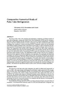
The possible failure modes in the tube hydroforming process are rupture, buckling, wrinkling and folding back. Rupture is the result of excessive internal pressure. Buckling, wrinkling and folding back is the result of excessive axial load. From these failure modes, a process window can be defined, see Figure 1.4. The process window is constructed in a diagram which has the internal pressure and the axial load on the axes. The lower boundary is set by the sealing force, i.e. the axial load needed to prevent leakage of the pressure fluid. The left boundary is defined by the internal pressure and the axial load needed to completely form the part. The upper boundary is the wrinkling limit. Here, buckling and folding back may also occur but in most cases wrinkling is the deciding factor. The right boundary is the rupture limit.

Axial load

wrinkling

process window

rupture

low pressure & low axial load leakage Internal pressure

Figure 1.4 The process window for tube hydroforming. Traditionally, the loading paths for the internal pressure and the axial load are determined by an iterative trial-and-error procedure. Past experience and simple equations are also tools for establishing loading paths. Axial feed for a specific part can, for example, be estimated by using volume constancy and assuming that the wall thickness of the formed part remains constant. In reality, however, it is almost impossible to maintain constant wall thickness due to the presence of frictional stress at the tool-tube interface and the variations in material flow over the entire deformation zone. The pressure loading path can be estimated by relating three pressure components; the yield pressure of the material, the rupture pressure, and the calibration pressure. From these three pressure components, a piece-wise linear curve can be constructed. Still, for complex parts estimated pressure curves may not agree with the 4

Introduction

process window, thus requiring expensive and time consuming trial-and-error based iterative procedures. The finite element simulation of sheet metal forming processes has been successfully applied to the analysis of real parts, a procedure denominated virtual verification. It is an interesting problem for researchers, since the battle between finite element models with calculation intensive equations yielding accurate results for complex problems and effective computational time is ever present. Efficiency is a very important factor in industrial applications of finite element simulations. Efficient solutions can usually be achieved by using elements based on simple theoretical assumptions. Fewer degrees of freedom in the element formulation, leads to faster calculations. Then again, the simplicity of the formulation must not be obtained at the cost of accurate results. Today, the explicit finite element method is the main tool for virtual verifications of tube hydroforming processes. Other methods are available but the explicit method is the most efficient method. An important characteristic of the explicit finite element method is the speed up of the simulation. This must be handled carefully. A too short simulation time may yield unreliable results due to unwanted dynamic effects. Hitherto, the simulation time is very conservatively set or based on experience to avoid complications. A desirable feature of a simulation tool would be the automatic generation of the loading paths for internal pressure and axial load. Today, these curves are preset for a finite element simulation and to find the optimal loading paths, many simulations must be performed. A solution to this problem would be to implement an adaptive loading procedure in the program. The adaptive simulation approach is based on the ability to detect/identify the onset and growth of defects during the process and promptly react to them. Loading paths can therefore be adjusted, within the same simulation run, to adjust the defects as defects tend to occur. If there is a risk for rupture, the pressure is decreased and the axial load is increased. And likewise, if there is a risk for wrinkling, the pressure and the axial load is changed accordingly.

1.2 Aim The aim of the thesis is to present a thorough literature survey of the tube hydroforming process and available simulation tools for the tube hydroforming process. Also investigate − adaptive loading algorithms − the boundaries of the process window − the speed up of the explicit finite element simulation.

5

Numerical simulation of tube hydroforming – adaptive loading paths

1.3 Limitations In the numerical modeling, the finite element method is used. The time integration is performed by an explicit scheme. The tube is treated as a shell and discretized into reduced shell finite elements. The forming process is considered as a process of large elastic-plastic strains and rotations. The material properties are described by an elasticplastic model for the work piece and a rigid material model for the die. Coulomb friction with sticking/sliding condition is assumed on the contact surface between the work piece and the dies. The simulations are not compared with physical experiments.

1.4 Contents Chapter 2 describes most of the hydroforming techniques in use today, for both sheet metal forming and tube hydroforming. The possible failure modes in tube hydroforming are also included. Chapter 3 contains the current knowledge of computational methods for sheet metal forming processes, including analytical methods, AI, statistical methods, optimization strategies, and of course the finite element method. The problem of establishing an adaptive loading procedure and its associated boundaries are presented. Chapter 4 reports of the implementations done by the author. An adaptive loading algorithm is tested. Two boundaries of the process window are established and varied with different simulation times. A method for detecting a too short simulation time is tried. In chapter 5, the thesis is brought to an end with a discussion. Some future research recommendations are made.

6

2

Hydroforming

Hydroforming follows from the principle formulated by Pascal in the 17th century when investigating the attributes of water - squeeze water and it squeezes back with equal pressure in all directions. Early investigations in the use of hydrostatic pressure showed the promise of increased ductility, thus making a sheet metal forming operation utilize the work piece better. Fuchs (1966) reported that in the beginning of the 20th century tensile tests were made on various materials while subjecting them to a hydrostatic pressure. The main result was that the ductility increased greatly, while the tensile strength of the material is increased only slightly. The formability of a material is enhanced. Despite the obvious advantages a hydrostatic pressure could offer in the metal forming industry, it would take many years before it was used - in the middle of the 20th century.

2.1 Sheet metal forming The sheet metal forming process, or deep drawing, is a widely used technique for producing parts from thin sheet metal blanks. The research has been extensive for many years and probably will be in the future also since the process is almost fundamental in our industrial world. This search for a more effective process, has given rise to a new technique, the hydroforming of sheet metal blanks. The prominent feature of this process is that the punch or the female side of the die can be dispensed with. The forming is the result of the pressure from a fluid. Depending on the shape of the product and field of application, different hydroforming techniques are applied. A comparison between conventional deep drawing and sheet metal hydroforming can be found in Kang et al. (2004).

7

Numerical simulation of tube hydroforming – adaptive loading paths

2.1.1 Conventional deep drawing The conventional deep drawing process is shown in Figure 2.1. It can either be applied in single or double action presses. The products can be used in a wide range of areas; for example cooking utensils (pots) or automotive parts, such as hoods, fenders, etc. Pots is an example of an easy drawn product since it is axisymmetrical, but in most cases the drawing is designed for a non-axisymmetric part which is a combination of deep drawing and stretch forming. To direct the metal flow between the binders, it is often necessary with additional features such as draw beads, lock beads, irregular shape of the blank and friction between the blank and the binders. Lubricants are used for decreasing the friction between blank and die. The blank holder is an important feature in the conventional deep drawing process. The magnitude of the force applied by the blank holder decides whether it will be a successful drawing or a failure by wrinkling or fracture. An insufficient force will result in wrinkling and too much force yields excessive stretching of the sheet or even fracture. The blank holder is not constricted to distribute uniform pressure along the blank. It can be designed that it exerts different magnitudes of pressure along the blank, a multi-point cushion. This is also used in the hydroforming process.

(a) single action presses

(b) double action presses

Figure 2.1 Conventional deep drawing in; (a) single action presses and (b) double action presses, Siegert et al. (2000).

2.1.2 Deep drawing process with fluid assisted blank holding In this process, see Figure 2.2, the blank holder is replaced by a fluid pressure usually with a rubber diaphragm between the blank and the fluid to prevent leakage. Otherwise, the process is as the conventional deep drawing. The friction is reduced considerably in the blank holding area. Shirizly et al. (1994) studies the role of die curvature and other properties for this process.

8

Hydroforming

Figure 2.2 Deep drawing with fluid assisted blank holding, Zhang and Danckert (1998).

2.1.3 Hydroforming deep drawing The hydroforming deep drawing process can be seen in Figure 2.3. The female die in the conventional deep drawing process is replaced by a counter pressure created from a fluid. A rubber diaphragm prevents leakage and the punch determines the final shape of the workpiece. The fluid pressure acts as a blank holder and prevents wrinkles. This technique is also referred to as soft-die forming. Numerous articles are investigating the forming limits, i.e. wrinkling and fracture. Yossifon and Tirosh (1985) investigate the maximum permissible fluid pressure before fracture. Yossifon and Tirosh (1988) continue the work in the previous article with the wrinkling limit and establish a safe zone for a permissible pressure path. Yossifon and Tirosh (1990) concern the maximum drawing ratio, i.e. when fracture and wrinkling are delayed till they occur simultaneously. Yossifon and Tirosh (1991) further investigate the fluid pressure path. Thiruvarudchelvan and Lewis (1999) perform tests with constant fluid pressure. An experimental study is done in Kandil (2003) and the results are also compared to conventional deep drawing. Soft-tool forming is the reverse hydroforming process, where the die is rigid and the fluid pressure acts as a punch, called Flexforming by ABB, Sweden, Ahmetoglu and Altan (1998). Bulge testing is often used as a means of determining material characteristics in engineering analysis. It is a soft-tool forming where the bulge formed by the fluid pressure does not meet any die surfaces. The blank is purely drawn to fracture. Finite element analyses are performed by Ahmed and Hashmi (1997, 1998).

9

Numerical simulation of tube hydroforming – adaptive loading paths

(a)

(b)

Figure 2.3 The hydroforming of a cylindrical cup; (a) Zhang (1999), (b) Thiruvarudchelvan and Travis (2003).

2.1.4 Hydromechanical deep drawing The difference between the hydroforming deep drawing process and hydromechanical deep drawing is the introduction of a mechanical blank holder, see Figure 2.4. As in conventional deep drawing, single or double action presses can be used, an example is the HydroMec System by SMG/Schuler in Germany. It is possible to pressurize the fluid in the beginning of the process, i.e. make a prebulging of the blank. This preforming of the workpiece makes it stiffer and less sensitive to dynamic denting due to the work hardening. It also feeds more material into the die for drawing of deep parts. Hsu and Hsieh (1996) do theoretical and experimental analysis for the hydromechanical deep drawing with a hemispherical punch.

(a) single action presses

(b) double action presses

Figure 2.4 Deep drawing with hydraulic counter pressure in; (a) single action presses and (b) double action presses, Siegert et al. (2000).

10

Hydroforming

2.1.5 Hydrodynamic deep drawing In the hydrodynamic deep drawing process, the fluid is allowed to flow out at high speed resulting in a rapid change of fluid pressure with the increase of the punch stroke. It is not necessary to control the fluid pressure and a rubber diaphragm is not needed. This process was introduced in 1958 as pressure-lubricated deep drawing and is also referred to as the Aquadraw process (ARMCO Steel Co, USA).

(a)

(b)

Figure 2.5 Hydrodynamic deep drawing; (a) Thiruvarudchelvan and Travis (2003), (b) Zhang and Danckert (1998).

2.1.6 Hydro-rim deep-drawing The hydro-rim deep drawing process can be seen in Figure 2.6. A fluid pressure is acting on the edge of the workpiece and reducing the tensile stress, in fact, feeding in more material and preventing an early fracture of the material. This deep drawing enhancement can be applied in both conventional sheet metal forming and hydroforming. Thiruvarudchelvan and Travis (1997) use this process in the redrawing of cups, thus improving the limit drawing ratio. Tirosh et al. (2000) studies the process and conclude, for example, that the process can be performed with a punch load equal to zero. Thiruvarudchelvan and Wang (1998) introduce a new hydraulic pressure aided technique, where the fluid pressure acts not only on the rim of the blank but also is the acting force behind two of the mechanical parts, the blank holder and the punch. The process is named hydraulic pressure augmented deep drawing. Thiruvarudchelvan et al. (1998), Thiruvarudchelvan and Wang (2000) and Thiruvarudchelvan and Wang (2001) further investigate this process. 11

Numerical simulation of tube hydroforming – adaptive loading paths

Figure 2.6 The hydro-rim deep drawing process, Tirosh et al. (2000).

2.1.7 Superplastic sheet metal forming process In the superplastic sheet metal forming, the blank is totally clamped between the binders, i.e. there is no flow of sheet metal. The pressure medium is a gas and the process is a warm forming process, see Figure 2.7. It is used when there is a need for products with excellent surface quality. Neutz et al. (2002) show the potential for gas to act as a driving media in deep drawing processes. The time for the deep drawing is much shorter than in the hydroforming process.

Figure 2.7 Superplastic sheet metal forming process, Siegert et al. (2000).

2.1.8 Viscous pressure forming Instead of a fluid, the viscous pressure forming uses a viscous medium that is strain-rate sensitive. This allows the pressure to be varied along the sheet, see Figure 2.8. The process is used for low volume stamping of difficult-to-form sheet metal alloys. Liu et al. (1996) perform FEM simulations of the forming process. Liu et al. (2000) make comparisons with the conventional punch forming. In Shulkin et al. (2000), the blank holder force distribution is investigated. 12

Hydroforming

Figure 2.8 Viscous pressure forming of a flat sheet blank: (a) during forming; (b) final forming stage, Zhang (1999).

2.1.9 Combination of conventional deep drawing and hydraulic pressure Using a combination of deep drawing and hydraulic pressure, the possibility of a deep drawing with controlled metal flow into the cavity is reached, see Figure 2.9.

(a)

(b)

Figure 2.9 Combination of conventional deep drawing and (a) hydraulic counter pressure, (b) hydraulic internal pressure, Siegert et al. (2000). 13

Numerical simulation of tube hydroforming – adaptive loading paths

2.1.10 Hydroforming of double blanks The hydroforming of double blanks is a process for forming hollow bodies. Hydraulic fluid is pumped between two blanks. The inner pressure forces the two blanks to move in separate directions towards the die. A preforming step can also be done by conventional deep drawing, see Figure 2.10. In Hein and Vollertsen (1999), many process parameters, such as load path and process window, are observed through experiments and numerical simulation. Novotny and Hein (2001) experiments with aluminum alloy sheets. Shin et al. (2002) are welding the blanks together at the edges. Novotny and Geiger (2003) perform experiments at elevated temperatures.

Figure 2.10 Hydroforming of double blanks, Siegert et al. (2000).

2.1.11 Integral hydrobulge forming (IHBF) Integral hydrobulge forming is a free hydrobulging process – the fluid is acting as the punch and there is no female die. The technique is suitable for forming special-shaped and specific-structured spherical and spheroidal shell products. Wang et al. (1989) introduces the process and a spherical vessel is formed from a welded polyhedron, see Figure 2.11. Zhang et al. (1996) replace the polyhedron with a single-curvature shell consisting of two polar flat circular blanks and several lateral roll-bent blanks welded into an oblate shell. Zhang et al. (1998, (1999) investigate the forming of double-layer spherical vessels. Zhang et al. (1999) form pressure vessel heads from circular flat plates.

Figure 2.11 A polyhedron, Wang et al. (1989). 14

Hydroforming

2.2 Tube hydroforming Depending on the time and country, the name for tube hydroforming has not always been the same. Bulge forming of tubes and liquid bulge forming were two earlier terms. Hydraulic (or hydrostatic) pressure forming was another form of name. Internal high pressure forming has been used and is used in Germany. In the language of solid mechanics, it is the biaxial stretching of the material by applying internal hydrostatic pressure. However, independently of its name, this metal forming process still has these basic features; a tube is formed into a complex shape with a die cavity using internal pressure. The pressure arises from a hydraulic or viscous medium, elastomers, polyurethane, etc. Simultaneously, an axial compressive load is often used, see Figure 2.12.

Figure 2.12 Hydroforming of an axisymmetrical part, Siegert et al. (2000). The technology of tube hydroforming has been present for at least half a century but it is only in the last decade of the 20th century that it has been firmly embraced by the industry. With the advancement of machine tools, high pressure hydraulic systems, sealing, work piece materials, lubrication and computer controlled processes, it has emerged finally as a viable sheet metal shaping technique and fit for mass production. Early products were used in plumbing and sanitary areas, for example tubular T-shapes (Figure 2.13). Today, tube hydroformed products have expanded into many more areas such as the automobile industry (exhaust system parts, chassis and body parts, engine components, etc). The term hydroformed part is nowadays often associated with the functions of ‘conveyance of liquid or gaseous media’ and ‘load transmission through components with a high load-bearing capacity and a low inherent weight’. The tonnage of a press depends on the product to be manufactured. Large components with thick walls and /or small corner radii need high closing forces. The capacity of presses has reached 10000 metric tons and they are operating at several plants in the world. The advantages are; (a) part consolidation (stamped and resistance welded two or more pieces of a box section can be manufactured in one operation from a hollow component), (b) weight reduction through more efficient section design and tailoring of the wall thickness, (c) improved structural strength and stiffness, (d) lower tooling cost due to fewer parts, (e) fewer secondary operations (no welding of sections required 15

Numerical simulation of tube hydroforming – adaptive loading paths

and holes may be punched during hydroforming), (f) reduced dimensional variations, and (g) reduced scrap. The drawbacks are; (a) slow cycle time, (b) expensive equipment, and (c) lack of extensive knowledge base for process and tool design.

Figure 2.13 The forming of a typical T-shape. Fa – axial force, Fq – counter pressure, Pi – internal pressure, Rc- corner radius, Re – fillet radius, Do – initial tube diameter, Dp – protrusion diameter, Hp – protrusion height, Lp – distance between tube edge and protrusion, Koc and Altan (2001). Characteristics of tubes are different than those of sheet metal from which they are formed since consequent rolling, welding and sizing operations alter the mechanical and micro-structural properties. Therefore, any measured data on sheet metal will not be useful for tubular materials even if they have the same grade and composition. Known and widely used material properties such as flow stress, strain hardening, anisotropy, yield strength, etc. will not be the same for sheets and tubes. In order to accurately analyze the tube hydroforming process, material properties directly measured on tubes should be used. Hydraulic bulge test is, for example, used to determine tube flow stress.

2.2.1 Hydroforming with internal pressure As early as in the 1940s, papers related to tube hydroforming were published. A patent was filed by Grey et al. (1939), concerning an apparatus using internal pressure and axial load for manufacturing copper T branches. Davis (1945) made experiments with tubes of medium-carbon steel under the combined pressure of inner pressure and tensile axial load. The research continued in the 1950s with Faupel (1956) and Crossland et al. (1959). The articles investigate the bursting pressure of thick-walled cylinders, experimentally and analytically. During the 1960s, more and more tests were conducted on thin-walled cylinders, accompanied by an analytical reasoning, for example by Mellor (1960), Weil (1963), and Woo (1964). Experimental studies on the expansion and flanging of copper tubes using hydraulic pressure is reported in Fuchs (1966). Ogura and Ueda (1968) inform about liquid bulge forming in Japan. A number 16

Hydroforming

of experimental results from the forming of T-shapes and multiple branch parts, for example bicycle frame junctions, using internal pressure and axial loading are presented. There is even a diagram of the formability region for a T-shape. In the 1970s, the research in both the experimental and the theoretical side of bulge forming expanded. New shapes, materials, bulging media, etc, are introduced. More sophisticated analytical investigations are applied and numerical solutions are introduced. In Al-Qureshi (1970), comparisons of polyurethane, rubber and elastomer working as the bulging media were performed. Woo (1973) continued on his work and formulated a numerical solution, using the finite difference method, when the tube, in its entire length, is in tension. Limb et al. (1976) made experiments with copper, aluminum, low carbon steel and brass for the forming of T-shaped tubular parts. The pressure medium was oil. In Woo and Lua (1978), the anisotropy effect were included in the analytical solution, which was compared to the experimental results. Hill’s theory of plastic anisotropy was used. Continuing with the 1980s, the research naturally increased. The determination of material properties and their effect on tube hydroforming interested researchers in Japan. Manabe et al. (1984) studied the tube forming using inner pressure and axial load with a computer-control system. The deformation behavior and limit expansion of aluminum tubes for a linear and nonlinear loading path were examined. In Fuchizawa (1984, (1987), material properties for tubes under internal pressure were investigated. The influence of the strain-hardening exponent on the limits of bulge height was presented. In the analytical work, incremental plasticity and membrane theories were utilized. Also, the influence of plastic anisotropy on deformation behavior was studied by placing the anisotropy in longitudinal or hoop direction. The analysis was based on deformation theory and Hill’s theory of plastic anisotropy. Later in the 1990s, Fuchizawa expanded the work by deriving stress-strain relations using membrane and plasticity theories and comparing these with experiments on aluminum, copper, brass, and titanium tubes, see Koc and Altan (2001). Ueda (1983) reports on the manufacturing of differential gear casings by liquid bulge forming. Entering the previous century, the experimental work and analytical derivations increased unabated. Numerical simulation of the tube hydroforming process became more and more important with the evolution of the computer. The finite element method is now used as a standard development tool after the multitude of investigations and validations done by researchers all over the world. In Thiruvarudchelvan and Lua (1991) and Thiruvarudchelvan et al. (1996), experiments with hydraulic bulging of tubes are performed. Some analytical comparisons are made. Thiruvarudchelvan (1994, (1994) uses an urethane rod as the bulging media and the analytical work is focused on the initial yield conditions. Sheng and Tonghai (1995) formed T-protrusions using a polyurethane pressure media and an axial compressive load. An upper bound method was employed to predict the total forming load. A new feature in the forming process was the use of a counter force. Bulging of tubes with internal pressure and axial load were carried out in Tirosh et al. (1996) and where the wrinkling and rupture failure were investigated, both experimentally and analytically. Sokolowski et al. (2000) describe a test method for determining the flow stress of tube 17

Numerical simulation of tube hydroforming – adaptive loading paths

materials. Prasoody et al. (2000) conducted experiments on extruded aluminum tubes in order to determine the forming limit diagram and the process window. Mac Donald and Hashmi (2000) study the forming of a cross-joint by finite element simulations. Mac Donald and Hashmi (2001) use LS-DYNA 3D to compare bulge forming with a solid medium against a hydraulic medium. In Ahmed and Hashmi (2001), two loading paths for the inner pressure were simulated in LS-DYNA 3D. Lucke et al. (2001) present the state of the art of the press technology and methods for process design. Manabe and Amino (2002) use LS-DYNA 3D for simulation of tube hydroforming and verify with experiments. Hsu (2003) used two CCD cameras in the experimental tests for measuring the deformation of a tube. Kridli et al. (2003) investigated corner filling by 2D simulations, using ABAQUS/Standard, and experiments. Kwan and Lin (2003) examine process parameters for the hydroforming of a T-shape using the FE program DEFORM-3D. Today, complex hollow parts are manufactured as the result of combining the hydroforming with preforming operations. The preforming can be a bending and/or a crushing process. The bending operation enables the tube to be placed in the die cavity. After that, the preforming by crushing is executed and it gives the advantage of having more material to work with or in other words, the tube walls lie much closer to the die sides and this gives a much more uniform thickness distribution. Another advantage of the crushing of tube is that the required inner pressure is much smaller, yielding smaller clamping force for the dies, which means that the press can be downsized. In the hydroforming cases with prebending, the axial feeding is not feasible or kept to a bare minimum. Ahmed and Hashmi (1999) made finite element simulations of the bulge forming of a pre-bent circular tube to square-sectioned elbow. Liu (2000) carry out consecutive finite element simulations of these operations for a cross member rail. Yang et al. (2001) compare different prebending operations using the FE-program PAM-STAMP. Hwang and Altan (2002) compare the processes of only hydroforming and the crushing plus hydroforming of tubes into triangular crosssections by FE simulations. Lee et al. (2002) do experimental studies of the bending, crushing and hydroforming of automobile radiator support members. Asnafi et al. (2003) perform the bending, crushing and hydroforming for automotive side members of extruded aluminum profiles and compare with FE simulations. Hwang and Altan (2003) compare the processes of only hydroforming and the crushing plus hydroforming of tubes in a rectangular die by FE simulations. In Dohmann and Hartl (1994), Dohmann and Hartl (1997), and Ahmetoglu and Altan (2000), necessary and important process parameters for tube hydroforming are presented along with finite element simulations. Gao et al. (2002) introduce a possible classification system for tube hydroforming processes based on process sensitivity to loading parameters. Historical overviews of the tube hydroforming process can be found in Ahmed and Hashmi (1997), Zhang (1999), and in the most comprehensive; Koc and Altan (2001).

18

Hydroforming

2.2.2 Hydroforming with external pressure For the forming of a tube onto a mandrel or the joining of two parts, a tube hydroforming with an outer fluid pressure can be preferred, see Figure 2.14.

(a)

(b)

Figure 2.14 Hydroforming with outer pressure; (a) tube formed onto a mandrel and (b) joining two parts, Siegert et al. (2000).

2.2.3 Hydroforming with both internal and external pressure A new technique for increasing the formability of a work piece is to apply the pressure both internally and externally. The increase in formability comes from the increase of the magnitude in the compressive through-thickness normal stress as a result of the presence of external pressure. Jain et al. (2004) carried out finite element simulations of the forming of an axisymmetrical part. Smith et al. (2003) combine this process with a preforming operation, crushing, see Figure 2.15. The forming process is simulated in a FE program with the use of different formability models, since the deformation history must be observed.

Figure 2.15 Tube hydroforming with preforming and both internal and external pressure; (a) tube and open die (b) closing die and crushing of tube (c) expansion, Smith et al. (2003). 19

Numerical simulation of tube hydroforming – adaptive loading paths

2.3 Failure modes in tube hydroforming There are mainly four types of failure in tube hydroforming; (a) rupture, (b) buckling, (c) wrinkling, and (d) folding back, which are all plastic instabilities in solid mechanics. Once such instabilities are started, they tend to persist and the stiffness of the specific area decreases. Therefore, deformation begins to be localized and eventually proceeds to final collapse or failure. As the formation of these instabilities is an important precursor to collapse or failure, computational prediction of the onset and growth of these instabilities is indispensable in understanding the final strength of the structures and materials, and in predicting and improving the formability. The failure modes which occur most frequently in tube hydroforming processes are rupture and wrinkling, see Figure 2.16.

Figure 2.16 Wrinkling and rupture failure, Asnafi and Skogsgårdh (2000). As long as the deformation is sufficiently small, the elastic-plastic boundary value problem has a unique solution which is referred to as the fundamental solution. When the deformation reaches a certain value, bifurcation from the fundamental solution becomes possible. The point of bifurcation can be found through the use of Hill’s general theory of stability and uniqueness for elastic-plastic solids, see Hill (1958). It is known that the failure modes in the physical hydroforming process arise from varying qualities of the work piece. This is true for the material properties as well as the geometry of the work piece. Unfortunately, the basic assumptions in most simulations, i.e. flawless homogeneous material properties and exact geometry of the work piece, do not reflect imperfections present in the physical world. The locations of these imperfections are often the instigation point of failure. In the finite element method, numerical conditions in adjacent nodes will not be the same and the difference in the numerical error, very small but still, will be the basis for failure. Tomita (1994) offer a review of plastic instabilities in solid mechanics with respect to numerical analysis.

20

Hydroforming

2.3.1 Rupture Rupture is a consequence of necking, which is a condition of local instability under the influence of large tensile forces. Once necking starts, the deformation becomes nonuniform throughout the part as it is under buckling and wrinkling cases. Deformation is concentrated in a local area, often denominated through-thickness necks. They are characterized by localized line thinning across the surface of the sheet with a width on the scale of the sheet thickness. Through-thickness necks proceed very rapidly towards fracture. The first stage of rupture is often induced by the presence of internal imperfections, such as micro-cavities and micro-cracks. The rupture failure is dependent upon process parameters, such as stress, strain, strain-rate, friction and forming temperature, as well as influential material parameters. The occurrence of necking or rupture is final and requires the rejection or redesign of the manufacturing process. This does not necessarily imply that the absence of said failure mode give an acceptable process. Normal process and material variations inevitably lead to necking and rupture during production runs. Prior to 1960, the only reliable test of formability in stamping and other sheet metal forming operations was whether or not the formed product was free of fractures and through-thickness necks. A reliable measure of forming severity that precedes these visible defects was necessary and, in a way, still is. Analytical studies of plastic instability (necking) can be found in Swift (1952), Hill (1958), Hillier (1963), Yamada and Aoki (1966), Chakrabarty (1969), Tvergaard (1990), Hill (1991), and Xing and Makinouchi (2001). The stability of long ductile cylindrical tubes under internal pressure has been the subject of several investigations. Storåkers (1971) analyzed rigid-plastic tubes and Chu (1979) elastic-plastic tubes subjected to internal pressure, in both cases in plain strain. In these studies, also very thin- and thick-walled tubes have been considered and all bifurcation points occur well beyond the maximum pressure point. If the internal pressure is prescribed, failure takes place in a circular cylindrical mode at the point of maximum pressure. If the prescribed parameter is the volume enclosed by the tube, cylindrical deformations may persist in a stable manner beyond the maximum pressure point until a bifurcation point is reached. Tvergaard (1990) include non-planar bifurcation modes. The first bifurcation into an axisymmetric non-cylindrical mode occurs just beyond the maximum point. This approach is in better agreement with the experimental results by Larsson et al. (1982). Simplified methods for rigid-plastic materials in plane stress are also available for tube hydroforming. From Hill’s uniqueness principle, the well-known diffuse necking criterion in Swift (1952) can be deduced, as explained in Yamada and Aoki (1966). The derived criterion was applied to the tube hydroforming process by Xing and Makinouchi (2001). A limitation for this type of method is that it does not take into account buckling of the tube under axial load. In Lei et al. (2001), some theories of rupture done by other researchers for the finite element simulation of sheet metal forming processes are mentioned. However, it seems that the various rupture criteria have a number of validity restrictions and that there are 21

Numerical simulation of tube hydroforming – adaptive loading paths

no universal criteria for metal forming processes. They implement instead the criteria proposed by Oyane et al. (1980) into an in-house implicit rigid-plastic finite element program. The loading path for the pressure is preset. Lei et al. (2002) and Lei et al. (2003) makes further simulations with this failure criteria. Boudeau and Gelin (1996) propose a method based on the linear perturbation technique to predict localized necking for the post-processing of finite element results of the simulation of deep drawing processes. Boudeau et al. (2002) extended this technique to a three dimensional stress state to be able to predict bursting during tube hydroforming simulations. Loading paths are not considered. Lejeune et al. (2003) continue using the method. Forming limit diagrams are built and the influence of material and process parameters on bursting predictions is studied.

Forming limit diagram The forming limit diagram (FLD), initially developed by Keeler and Backofen (1963) and Goodwin (1968), provides a useful empirical gauge of forming severity in the absence of a neck or split. The FLD represents the relationship between the limiting major and minor principal strains in the plane of the sheet prior to the onset of localized necking. The key feature of the FLD is an experimentally determined forming limit curve (FLC). The shape and location of the FLC, which defines the boundary between strain states that are always free of necks from those states that are prone to necking and splitting, are characteristics of the metal that is independent of the forming process or work piece shape. Therefore, the distance between the FLC and all of the measured or predicted strains throughout the formed part characterizes the degree of safety. For example, Figure 2.17 shows the FLC for an aluminum alloy as reported by Graf and Hosford (1993). A corresponding safety margin is often defined by a fixed offset from the FLC as a design criterion to develop robust forming processes under the variability of the manufacturing environment. The FLD is very useful in FEM analysis, die design optimization, die tryout, and quality control during production. Asnafi and Skogsgårdh (2000) show that the forming limit diagram of the tube material must be determined by hydroforming if the component and process design are to rely on the FLD to predict the onset of necking.

22

Hydroforming

Figure 2.17 Forming limit diagram for 2008 T4 aluminum in the as-received condition. The solid line is the experimental forming limit curve and the dashed ling illustrates the conventional safety margin curve used as a maximum strain criterion in die design, Graf and Hosford (1993). Two main methods of calculating the forming limit diagram analytically are present today. One is called M-K analysis, first postulated by Marciniak and Kuczynski (1967), with the hypothesis that localized necking initiated from a pre-existing material imperfection which was represented by a thinned linear region. The failure can be defined to occur when the incremental change of ε1 outside the weak region, ∆ε1a, is less than or equal to one-tenth of that inside the weak region, ∆ε1b, while the imposed ∆ε2a and ∆ε2b are equal. The calculated FLDs were found to be sensitive to the imperfection parameter and the material model, such as the initial yield surface shape (in e.g. Cao and Boyce (1997)), strain hardening (in e.g. Marciniak and Kuczynski (1967)), strain rate sensitivity (in e.g. Neale and Chater (1980)), and plastic anisotropy (in e.g. Cao and Boyce (1997)). Friedman and Pan (2000) combine the M-K analysis with three different yield criteria and study the effect on the right hand side of the FLD. Cao et al. (2000) use a combination of M-K analysis and a general anisotropic yield criterion to predict localized thinning of sheet metal alloys for linear and nonlinear strain paths. In most cases, the M-K analysis makes an overestimation in the region close to equi-biaxial stretching. The second approach for calculating the forming limit diagram is the classical bifurcation analysis initially proposed by Hill (1952) and extended by Storen and Rice (1975) and later by Hutchinson and Neale (1978) in conjunction with using deformation theory. Hutchinson and Neale (1978) also applied deformation theory to the M-K analysis using von Mises yield criterion and showed that the FLC predicted by the flow theory with a smooth yield surface, especially in the

23

Numerical simulation of tube hydroforming – adaptive loading paths

biaxial tension region. The results based on deformation theory were in much better accordance with experimental results. The problem with the FLD is that it is valid only in processes in which the loading path is linear; in other words, one in which the ratios of the plastic strains are constant throughout the forming process. The seriousness of this problem is illustrated in Figure 2.18, which shows the dependence of the FLC on 15 different bi-linear loading paths as reported by Graf and Hosford (1993) for 2008 T4 aluminum. The first segment of the dashed lines in this figure represents the strain increment during the first loading stage in one of the Graf and Hosford tests. The second segments of the dashed lines, which are almost vertical in this diagram, connect the end point of the prestrain to the associated experimental FLC. These FLC’s show the strain level at which necks are observed in a subsequent linear loading path along a different direction. This dependence of the shape and location of the FLC on strain path is typical for all materials including steel alloys, copper, and brass, as reported, for example, by Kleemola and Pelkkikangas (1977).

Figure 2.18 Changes to the forming limit curves after prestrain to several levels of strain in uniaxial, plane strain, and equibiaxial conditions. The dashed lines emanations from origin show the prestrain path for each condition, with the second leg showing the plane strain path of the secondary forming operation to the associated forming limit curve, Graf and Hosford (1993). Strain path effects undermine the utility of the traditional strain-FLD for formability assessment of secondary forming processes such as re-strikes and flanging operations, where the strain path in the second process is independent of the path during the first process. It also inhibits its utility for analysis of processes that are inherently non-linear, 24

Hydroforming

such as tube hydroforming. Furthermore, experience shows that non-linear strain paths play a role in complex first draw forming processes, particularly when re-entrant tool surfaces caused by pockets and other features, contact the sheet late in the process and change the direction of metal flow. Occasionally, these strain path changes are significant enough that the conventional FLD gives a false measure of forming severity even in the first draw die. Failure to detect these formability problems early in the design process leads to substantial increases in die cost, which continues to be a major factor in the overall cost of parts manufactured from sheet metal. The challenge with the strain-path effect is that each point on the product is subjected to a different strain path and so requires its own unique FLC. Obtaining these FLC’s is far more difficult than modifying the experiments, as Graf and Hosford (1993) did show in Figure 2.18. This figure shows what happens to the FLC when the strain path is bi-linear and the principal stain axes of the two linear segments are not rotated with respect to each other. In a complex stamping or multi-stage forming process, the strain path varies throughout the forming operation, changing not only the ratio of the strain increments, but also the direction of these strain increments with respect to the material axes. The number of required FLC’s to deal with the general problem is practically limited to the number of elements in the FEM analysis or the number of grid circles on the panel, but it may as well be infinite. Taking into account the strain-path dependence using experimental FLC’s for each point in a complex stamping operation is unrealistic. Some other method is required. Obermeyer and Majlessi (1998) give a brief historical background of how and why the formability of sheet metal is defined in terms of a two-dimensional strain map. It also describes how the measure of formability depends on the state of strain, which in turn depends on the specific experimental technique used. The research work dealing with both experimental and theoretical determination of the forming limit diagram is reviewed, the focus being to demonstrate the significance of the strain path on the FLD by showing how the calculated limit strain depends on the strain history. Stoughton (2000) presents a forming limit criterion based on the state of stress. Darlington et al. (2000) do experiments with tubes and discuss the forming limit curves based on strain and stress. Stoughton and Zhu (2004) review the strain based FLD and present the stress based FLD.

2.3.2 Buckling/wrinkling Buckling of tubes can be analyzed in two groups as occur in the physical world – global and local buckling. The global buckling is the buckling of tubes as a column and the local buckling is defined as the wrinkling of tube walls. Buckling represents a stability problem. The axially loaded specimen deforms so that the new geometry, from a mathematical point of view, is in a stable state of equilibrium. By continuous increase of the force, the state of equilibrium is formally maintained, but at a certain time it becomes unstable. At this critical point, even the smallest disturbance such as noncentered point of application of force, inaccuracy due to manufacturing, etc, will lead to instability. This holds for a buckling of a bar as well as for the wrinkling of sheet metals. Previously, the engineer’s duty was to avoid wrinkles, since a drawing piece 25

Numerical simulation of tube hydroforming – adaptive loading paths

with such a geometry cannot fulfill the requirements of the design nor its original function. Considering the tube hydroforming process, small wrinkles can be allowed during the process since they can be suppressed and made to disappear during the calibration using the inner pressure.

Buckling The danger of buckling occurs at the start of the operation as a result of an excessively high axial force acting on the undeformed tube. The permissible buckling force at the start of the process can be estimated in theoretical terms. The buckling of a tube is essentially investigating the applicable Euler case, case number four where both ends are fixed. The Euler formulas are valid in the elastic range and are often expanded into the plastic range by using the tangent modulus, Et, instead of the modulus of elasticity, E. However, the danger of buckling must also be countered beyond the beginning of the operation, throughout the entire start-up phase. An attempt must be made through an appropriate form of process control to ensure that the reduction in the free length of the tube achieved through compression is accompanied by a rapid increase in the section modulus of the tube cross-section over the entire length of the expanded tube where possible, see Figure 2.19 and Dohmann and Hartl (1996).

Figure 2.19 Buckling stress σz, tangent modulus Tp, and section modulus Jz in relation to the expansion of the tube, Dohmann and Hartl (1996).

Wrinkling Wrinkles are short-waved out of plane deformations. Whenever a sheet is in a state of in-plane compression there is a potential risk for wrinkles. The general theory of bifurcation and uniqueness by Hill (1958) built a foundation for much of the subsequent research on wrinkling. Hutchinson (1974) detailed the bifurcation theory for structures where the material is in the plastic range. At the onset of wrinkling, there 26

Hydroforming

are at least two possible solutions – the unwrinkled state and the wrinkled state. At this point, the inequality is violated and the solution is non-unique. The theory is essentially an eigenvalue problem and bifurcation is possible at the lowest eigenvalue of the bifurcation function. Hutchinson and Neale (1985) later extended the theory to the conditions needed for the onset of wrinkling in a doubly-curved sheet metal without lateral constraint. It was deduced that wrinkling is most likely a local instability problem depending on the local curvature and local stress states. This finding applies to plates and shells whose top and bottom surfaces are free of contact. The problem differs slightly when considering the effect of a lateral constraint (constraint normal to the plane of the sheet) on buckling. In the case of sheet metal forming, lateral constraints are present in the form of blank holder/sheet/die or die/sheet/die interactions where the sheet is constrained to some extent between a blank holder and a die or matching dies via a force-controlled or displacement-controlled condition. Experimental and numerical investigations show that wrinkling behavior depends on the pressure applied normal to the sheet by the blank holder, as well as the local stress states and curvature. In Triantafyllidis and Needleman (1980), an analytical solution was derived for this situation. The bifurcation theory was applied to an annular plate subjected to axisymmetric radial tension along its inner edge. By resting the annular plate on a continuous linear elastic foundation, the blank holder is treated as a deformable blank holder. The effect of blank holder stiffness on the critical buckling stress and the wave number is obtained. Small strain deformation is assumed. Tvergaard (1983) analyzed the wrinkling of elastic-plastic shells subjected to a compressive axial load, where the influence of various geometric and material parameters was studied for a wide range of radius-to-thickness ratios. J2-flow, J2deformation and J2-corner theories were used and compared. Simultaneous analysis of bursting and wrinkling is not easy to achieve. Experimental results on short tubes in Tirosh et al. (1996) are guided by a limit analysis formulation. Xia (2001) develops a simplified analytical method for tubular hydroforming under internal pressure and end feeding. Bursting and wrinkling are considered as distinct failure modes and diagrams of the process window for different materials are presented. Different loading paths are simulated and the results are compared with the result of the analytical solution which must have a proportional loading path. Swift (1952) gives two criteria for sheet metal forming that can be applied to tube hydroforming, but for different loading cases. More precisely, if internal pressure and axial compression are independent, Swift’s usual criterion does not apply. In both cases, Swift’s criteria do not take the buckling load into account and it can be shown, that the limit strain for buckling is much smaller than the limit strain for necking, see Nefussi and Combescure (2002). Nefussi and Combescure (2002) discuss the hydroforming limits (necking and wrinkling) of isotropic tubes subjected to internal hydraulic pressure and independent axial load, analytically and numerically. The loading path is not considered. Xing and Makinouchi (2001) use Hill’s general theory for the uniqueness in the boundary value problem to investigate how different parameters influence the plastic 27

Numerical simulation of tube hydroforming – adaptive loading paths

instability in the tube hydroforming process. The classical lines in the tube hydroforming limit graph are corresponding to the special positions in the yielding locus, shown in Figure 2.20. This figure also shows the strain state of the plane stress processing proposed by Wang. No thinning of the thin-walled tube occurs when the deformation path is between paths 4 and 6, and the closer to position 6 it gets, the thicker it is. There may exist wrinkling due to the axial compression stress when the deformation path is between paths 3 and 6. Thus, if the deformation path is designed from the higher axial compression zone to the lower or the biaxial tensile one in the arrowed zone in Figure 2.20, it will give a higher forming limit in the higher axial compression zone. This means, that the generation of moderate recoverable wrinkles in the earlier free forming stage is a benefit. It prevents the tube from over-thinning and all wrinkles are removed in the later stage.

Figure 2.20 Stress-strain state of tube hydroforming, Xing and Makinouchi (2001). A much more comprehensive study of the wrinkling phenomena is presented in the next chapter since wrinkling is a basis for loading path determination in this thesis.

2.3.3 Folding back Folding back occurs when the axial load is excessively increased after wrinkling has been recognized. The tube folds back on itself. It can also happen when the geometry is complex, e.g. in a T-branch hydroforming process. The material flowing through the radii into the protrusion disconnects from the die wall and proceeds toward each other due to the axial load. In this case, wrinkling has not occurred. Folding back is an irreparable failure and should be fully avoided. 28

3

Computational methods

Predicting the behavior of a sheet metal forming process is very difficult. Many factors must be considered, e.g. non-linearity of material properties, friction effects at the die/workpiece interface, nonsymmetrical dies, etc. The analytical procedure may be sufficient for symmetrical and simple forming processes. However, the complexity of the mechanics of these problems is still considerable. For a realistic computation of the forming process, numerical methods for computers must be utilized. The main numerical method today is the finite element method. In any design of a new structure or process, there is need for verification. The verification process is an important part of the quality work. Traditionally, this is done by physically building the structure and testing it repeatedly, varying important parameters. The process is very time consuming and expensive. The last decade this has changed, due to the improvement in the computer and the software business. Nowadays, the verification is done by running a sophisticated calculation program in a computer, making the physical testing almost obsolete. This is called virtual verification.

3.1 Virtual verification The role of experiments has changed with the increasing opportunity of making simulations of various investigations, e.g. design, optimization, parametric studies, etc. Nowadays, experiments are used sparingly and primarily in the following areas; creating material and friction models, verify computer simulations and final prototype verification, Eriksson (2000). The virtual verification process contains a number of stages which can be combined into a circle, see Figure 3.1. It begins with the data collection, which can be handled electronically and/or physically. Continuing with the preprocessing stage, a file from CAD/CAM is used as input. The model is then divided in elements - meshing of the 29

Numerical simulation of tube hydroforming – adaptive loading paths

model. Material parameters and other important criteria, e.g. contact surfaces and loads, are defined. Now the model is ready for the simulation. This is either done by an onestep reverse solver or an incremental solver, depending on how far into the developing process the model is. The output from the simulation is then examined in a postprocessing program, often using a forming limit diagram. Then the optimization process begins. Geometry, thickness and process parameters are varied so that the final result will satisfy the design criteria. A final simulation is done with the incremental solver for the virtual verification. The dies are manufactured according to the results from the simulations and forming experiments are performed. Strain analyses are commonly done for the verification of the simulation results. The results and experience attained are then stored in a database at the end of the design process as a support for new products. Data support

Verification

Data collection

Preprocessing

Optimization Simulation Postprocessing

Figure 3.1 Methodology of virtual verification. A survey conducted at Volkswagen (Svensk Verktygsteknik (2001)) gives an idea of the proportional amount of time spent in the various virtual verification stages. The last two stages are not accounted for in the survey, see Table 3.1. As can be seen, 80% of the work is done in the first three stages - collecting data and preprocessing. This signifies how important correct input parameters are considered. The accuracy of the output depends on how well established the input parameters are.

30

Computational methods

Table 3.1 Time spent in the virtual verification process. Stage

%

Collect data

40

Prepare input

20

Create models 20 Simulation

15

Study output

5

Several softwares are available for simulating forming processes, e.g. LS DYNA3D, ABAQUS, PAM-STAMP, MARC, AUTOFORM, DEFORM, etc. Some are very extensive, capable of simulating most problems in continuum mechanics. Some are more or less adapted to the special circumstances in forming processes. In the process of creating a product, the engineer is using two different simulation programs - an onestep reverse solver and an incremental solver. The following figure, Figure 3.2, shows when in the creating process the specific solver is used in a die design.

Onestep reverse solver

Early analysis

Construction of die

Early model

Design of product

Die design

Design of process

Incremental solver

Verification

Die production

Mounting

Figure 3.2 The design process, Svensk Verktygsteknik (2001). The one-step reverse solver has as input the finished part. The solver then “flattens” the part to a sheet, i.e. the simulation does the forming process in reverse order. The solving algorithms are much simpler than incremental algorithms, hence spending less 31

Numerical simulation of tube hydroforming – adaptive loading paths

computational time. The one-step reverse solver is used early in the design process. The process and geometry in the specific forming operation can still change a lot. The solver gives a rough estimate of the feasibility of forming the part. Nguyen et al. (2003) and Nguyen et al. (2003) study an inverse analysis, i.e. one-step reverse solver, for tube hydroforming and compare with results from the FE program MARC. The incremental solver is the conventional FE-program. It can be either an explicit or an implicit based solver, though explicit seems now to be the predominant solving technique in forming simulations. Even though virtual verification, or virtual process simulation, greatly reduces the development time and prototyping cost, a lot of time is consumed in the trial-and-error work of optimizing a tube hydroforming process. Systematic procedures and use of optimizing techniques can reduce the engineering effort and lead times required by simulation. Still, in order to shorten the design process time for the tube hydroforming process, supplemental codes and techniques are being developed, e.g. adaptive techniques. Strano et al. (2004) discuss strategies for improving the work performed during the virtual verification stage in tube hydroforming.

3.2 The finite element method The finite element method is the most accepted technique for numerical simulation of sheet metal forming processes. In early work in the 60s and 70s, other numerical methods were also in use, e.g. the finite difference method. Woo (1968) compared the experimental results of a deep drawn cylindrical cup with a numerical solution. The numerical method was based on a rigid-plastic finite difference membrane model. Since the finite element method basically is numerical calculations, it is directly coupled to the capacity of a computer. This give, that for a long time simplifications were made, and still are but not in such wide extent, in the simulations of sheet metal processes. The simulated forming process was predominantly axisymmetrical or twodimensional. Koc and Altan (2002) demonstrate the use of two dimensional finite element analyses and its place in the design process. DEFORM2D were used and compared with simulations from LS-DYNA3D. Even though the results of two dimensional analyses are approximate, it is useful at the initial phases of designing a new part for the tube hydroforming process. Rama et al. (2003) present a two dimensional numerical method for analyzing the tube hydroforming process. It includes also an approach to predict the loading path of the inner pressure. Different theories for the material models have been developed over the years. The most common is the elastic-plastic model, i.e. non-linear elasticity theory. Another is the rigid-plastic model, where the elastic deformation is neglected. Chiang and Kobayashi (1966) utilized a rigid-plastic model for deep drawing. Other fundamental material models for sheet metal behavior exist, e.g. the elastic-viscoplastic and the rigidviscoplastic. The viscoplastic flow formulation is stated as analogous to standard nonlinear elasticity theory. The former in; Takezono et al. (1980) simulates thin circular plates using a elastic-viscoplastic finite element solution with membrane shell theory. 32

Computational methods

The latter can be found in; Onate and Zienkiewicz (1983) present a viscous shell formulation for sheet metal forming. The general viscous shell element is derived from the standard reduced integration, “thick” shell element. A brief historical review of the finite element method is also included. In Onate and Agelet de Saracibar (1990), bending/membrane viscous shell elements are derived. These elements are then selectively used in various parts of the sheet, depending on the nature of the deformation. Sosnowski et al. (1992) compare experimental tests with the numerical simulations. The numerical code is based on a finite element viscous shell approach. Sukhomlinov et al. (1992) describe an axisymmetric rigid-viscoplastic finite element membrane model. Doege et al. (1996) present constitutive models for anisotropic behavior, ductile fracture analysis using the Gurson model, and phase transformations due to for example welding. The implementation is done in ABAQUS. The full three dimensional solution of a sheet metal forming process is very expensive in terms of computational time. Using three dimensional elements for the solution obviously would be too time-consuming. In early work, axisymmetric solid elements were utilized. Since the process consists of thin sheet metal, certain assumptions are valid, e.g. plane stress, and shell theory can be applied. Still, further assumptions are made and many different shell element theories are spawned. The membrane element is the cheapest shell element in terms of computer cost and was used extensively in the development of the finite element method for sheet metal forming processes. Membrane theory does not include the variation of stresses through the element thickness and cannot handle the bending stress. These bending stresses must be considered when dealing for example with spring-back. Several shell elements have been derived using a reduced integration scheme for the purpose of making the solution faster. These elements are efficient but they have one crucial drawback – hourglass modes are not detected and non-physical features must be introduced in the formulation. Wifi (1976) used axisymmetric elastic-plastic solids in the finite element method. Wang and Budiansky (1978), and Tang (1981) derived each an axisymmetric elastic-plastic implicit finite element membrane model. Hsu and Chu (1995) give a small historical review of the numerical simulation in sheet metal forming using membrane theory. An axisymmetric elastic-plastic implicit finite element membrane model was developed for the analysis of sheet metal forming processes. Rojek et al. (1996) derive continuum and shell elements for the explicit finite element method. Continuum elements offer the possibility to use a more exact three dimensional description of the deformation and allow better consideration of two face contact considerations, but it is not as numerically efficient as the shell element. Rojek et al. (1998) present a triangular element for forming simulations, an implicit finite scheme for springback simulation, and parallel processing for computational efficiency. Lange et al. (1991) give an account of an implicit finite element program with an elastic-plastic material model. By using axisymmetry, the simulations were done in two dimensions. A variety of element types were applied in the simulations. Hutter et al. (2000) present a total Lagrange hourglass control which is physically based and contains no estimation of an empirical factor. Galbraith and Hallquist (1995) examine the seven four-nodal shell elements in the explicit finite element program LS-DYNA3D (version 920) from a cost-benefit point of view. 33

Numerical simulation of tube hydroforming – adaptive loading paths

Today, the computer power is at such a level that fully three dimensional models can be considered. As stated earlier, the simplifications of a real three dimensional structure is the result of inadequate computational power. A consequence of the simplifications is a probable loss of accuracy in the simulation results. Thus, finite element simulations with three dimensional elements are desirable. Nevertheless, simple shell theory should not be discarded so easy yet. Shell elements are computer efficient and by increasing the number of elements in the mesh, the accuracy of the solution is increased. Menezes and Teodosiu (2000) present an implicit finite element method with three dimensional elastic-plastic elements. In Lei et al. (2000), an in-house finite element program with three dimensional rigid-plastic elements, HydroForm-3D, simulates the hydroforming of an automobile rear axle housing. Lei et al. (2001) also use this FE-program for a variety of tube hydroforming processes. Kim and Kang (2002) implement a backward tracing scheme to the program for determining the starting conditions from the final configuration. Kim et al. (2002) are also dealing with the backward tracing scheme. Kim et al. (2002) evaluate a new contact algorithm for the program and simulate the forming of an automobile lower arm. In Kim et al. (2002), the numerical results are compared with experiments. Kim et al. (2003) is a continuation of previous papers. Lei et al. (2003) describe the implicit rigid-plastic FE program theoretically and make some simulations. Even with the powerful computers of today, the search for numerically cheap algorithms and theories are ever present. The most effective means of achieving this is to reduce the degrees of freedom, i.e. use shell elements instead of three dimensional solid elements. The last decade, the explicit formulation has been the most popular time integration method but research is also done for the implicit formulation.

3.2.1 Dynamic finite element formulation The differential equation governing the motion of a material point is

σ ij , j + ρ bi = ρ ai

(3.1)

σ ij n j = t i on S1

(3.2)

ui = ui

(3.3)

on S2

where σij is the Cauchy stress tensor, ρ the current density, ai the acceleration, bi the body force density, ti the given surface traction, ui the displacement boundary condition, and nj the unit outward normal to the boundary surface. The variational equation is then given by

∫ ρ a δ u dV + ∫ σ δ u i

V

34

i

ij

V

i, j

dV − ∫ ρ biδ ui dV − ∫ t iδ ui dS = 0 V

S1

(3.4)

Computational methods

where δui is an arbitrary variation of the displacement field compatible with the boundary conditions. Spatial discretization is performed with n elements and then the finite element equation is obtained as n

⎧⎪

⎫⎪

∑ ⎨ ∫ ρ N NadV + ∫ B σ dV − ∫ ρ N bdV − ∫ N tdS ⎬ = 0 m =1

⎩⎪Vm

t

t

Vm

t

Vm

t

S1

⎭⎪

(3.5)

where N is the interpolation matrix and B the strain-displacement matrix. Two types of non-linearity occur in the numerical simulation of the hydroforming process, actually in every sheet metal forming process. One is the large elastic-plastic transformation and the other is contact conditions. The two types of non-linearity are interrelated, i.e. changes in one affect the other and vice versa. Two techniques for dynamic finite element calculations are present – the implicit and the explicit formulation. In implicit methods, the configuration at t+∆t is found from expressions that involve F=ma equations written at time t+∆t. In explicit methods, the configuration at t+∆t is found by the use of F=ma equations written at time t. Explicit integration require a small ∆t but have equations that are cheap to solve, while implicit integration allow a large ∆t but uses equations that are expensive to solve. The implicit finite element method provides a more reliable and rigorous scheme when considering the equilibrium at each step of the deformation. The major obstacle for the implicit formulation lies in the cases when converged solutions cannot be achieved due to the changing contact and friction conditions. There is also the concern for the great time consumption in the handling of contact conditions and the solution of large system of equations. The advantage of the explicit formulation is in the superior handling of the fast changing boundary conditions for complex die surfaces. Explicit time integration is numerically efficient with low memory requirements and easy treatment of contact conditions. Mattiasson et al. (1991) compared the explicit code DYNA3D with the implicit code ABAQUS and made experimental verifications for sheet metal forming processes. Yang et al. (1995) made a comparative investigation of implicit, explicit and iterative implicit/explicit schemes for the simulation of sheet metal forming processes. Onate et al. (1995) compare quasi-static viscoplastic flow and elastic-plastic solid models and explicit dynamic models for the simulation of sheet metal forming processes. Kim et al. (2002) compare an in-house implicit program and LS-DYNA3D for the tube hydroforming process of an automobile lower arm. Also, a guideline for establishing the simulation time in the explicit case is proposed. Cao (1994) describes a semi-implicit scheme for deep drawing simulations. For each time increment, an initial guess of the solution is obtained by using a tangent formulation. After choosing the increment of the loading parameter, the configuration and the state of the sheet are updated in an explicit way. Then, an implicit algorithm is used to ensure equilibrium, under constant status of the contact nodes and for fixed values of the loading parameter. Finally, the boundary conditions are adjusted to the 35

Numerical simulation of tube hydroforming – adaptive loading paths

new values of the contact forces and to the new positions of the nodes. In Finn et al. (1995), the explicit LS-DYNA3D is coupled with the implicit LS-NIKE3D for efficiently predicting the springback in sheet metal forming. The explicit program is suitable for the forming process and the implicit program, subsequently model the springback. Taylor et al. (1995) also investigate when the explicit and the implicit finite element program, ABAQUS/Explicit and ABAQUS/Standard, are put to best use in sheet metal forming simulations. Cherouat et al. (2002) use the explicit scheme (ABAQUS/Explicit) to solve the global dynamic equilibrium problem while the implicit scheme is used for local time integration of the constitutive equations in tube hydroforming processes.

Implicit formulation In the implicit formulation of the finite element method, the structural balance is ensured at any given instant of the calculation. The known configurations at instant t are transferred to the instant t+∆t and the equilibrium equations are solved. The static structural balance is assured by an iterative scheme in the vicinity of the arrived configurations at instant t+∆t. The algorithms are much more sophisticated than in the explicit method and allow for greater time increments. Most implicit time integrations are unconditionally stable, which means that the size of the ∆t is governed by considerations of accuracy rather than stability. On the other hand, it has some disadvantages compared to the explicit method. The implicit algorithms have no protection against eventual numerical instability and divergence can occur during the iteration process. In general, this is associated with severe changes in the boundary conditions or in the strain evolution during an increment. In the implicit method, equilibrium equations and the coherence condition are imposed on the configuration at the instant t+∆t, which is unknown. This configuration has to be determined by successive approximations. The correction of the solution comes from the iterative Newton-Raphson method and direct iteration methods. The direct iteration method is used to generate a good initial guess for the Newton–Raphson method, which is used for speedy final convergence. Esche et al. (1997) focuses on techniques to overcome numerical difficulties, e.g. convergence, in implicit finite element programs.

Explicit formulation The treatment of the deformation in an explicit finite element simulation is quasi-static, since the equation of motion is fulfilled only at discrete time intervals, ∆t. At these discrete time intervals, in principle a static equilibrium is obtained and static analysis tools are available for calculating the new configuration. The explicit procedure requires no iteration and no tangent stiffness matrix. Efficiency is achieved when diagonal element mass matrices are used, i.e. lumped mass matrices. By mass lumping of the first term in equation (3.5), the uncoupled finite element is obtained as 36

Computational methods

Ma = F ext − F int

(3.6)

ext

where F is the nodal force vector resulting from the surface traction and the body force, Fint the nodal force vector resulting from the stress divergence and M the lumped nodal mass matrix. The term lumped means that the elements are condensed on the diagonal. The central difference method is used to integrate the equations of motion an = M n−1 ( Fnext − Fnint )

(3.7)

vn + ½ = vn −½ + an ∆t n

(3.8)

un +1 = un + vn +½ ∆t n +½

(3.9)

∆t n + ½ =

1 ( ∆t n + ∆t n +1 ) 2

(3.10)

where v and u are the global nodal velocity and displacement vectors, respectively. The geometry is updated by adding the displacement increments to the initial geometry. The explicit time integration is conditionally stable. It can be shown that the stability limit for the time step approximately is ∆t < ∆t cr ≈

L Cd

(3.11)

The critical time step, ∆tcr, is the shortest length of an edge in the finite element mesh, L, divided by the dilatational wave speed of the material, Cd. If the time step does not conform to this criterion, computed displacements and velocities grow without limit. Hallquist et al. (1995) give an overview of adapting the explicit finite element program LS-DYNA3D for parallel computers and the suitability of using this program for sheet metal forming applications. The structure of explicit finite element programs with diagonal mass matrices makes them appropriate for parallelization and vectorization.

3.2.2 Concepts of time Three different time concepts are used in connection with explicit finite element simulation of sheet metal forming operations – the process time, the simulation time, and the computational time. The process time is the real time used in a manufacturing machine to produce a part. The simulation time is the fictitious time used for application of forces and boundary conditions in the computer simulations. The computational time is the real time used for the computer simulations. The process time is usually 0.5-10 seconds, the simulation time is in the range 10 milliseconds (ms) to 300 ms and the computational time is from 1 hour to a week, depending on computer and model size.

37

Numerical simulation of tube hydroforming – adaptive loading paths

For typical sheet forming operations, the time step is in the order of one microsecond. Since the process time is in the order of one second, millions of time steps are required for a simulation run. A standard approach of reducing the computational time is to model the forming process as if it occurs in a shorter time, i.e. using the simulation time. Another way achieving this speed-up of the process time is to change the mass of the moving parts in the forming process. An increase of density of the material by a factor x will decrease Cd in equation (3.11), thus increase the time step by the squareroot of x. There is a limit for the speed-up. The kinetic energy of deformation must be kept below a certain level so that the dynamic effect in the simulation is negligible. With appropriate care, accurate solutions should be possible for sheet metal forming processes. Chung et al. (1998) suggest an energy error estimate for how close a sheet metal simulation is to a static process, i.e. the error due to dynamic effects. It could be a useful input for the choice of simulation time. Kutt et al. (1998) investigate the effects of speeding up the deep drawing process and also study the consequences of different shapes of the punch load curve. The two dimensional simulations are done in NIKE2D and DYNA2D.

3.2.3 Contact analysis In LS-DYNA3D, the contact interface consists of a master surface and a slave surface. The contact algorithm performs a so-called slave search which means that the algorithm checks for penetration of slave nodes into the master surface, see Figure 3.3.

Slave

Master

Figure 3.3 Penetration of three slave nodes and application of interface forces.

When the slave nodes and the corresponding master segments are identified, the contact algorithm may proceed according to several different schemes. A widely used method is the penalty procedure. It gives a smooth initial impact and minimal disturbance to the mesh. The penetration of nodes is prevented by the application of artificial springs between the penetrating slave nodes and their corresponding master segments. The interface force to a slave node is calculated from the supposed penetration length and an interface stiffness based on the bulk modulus and the

38

Computational methods

dimension of the element. The slave nodes which have penetrated are relocated to the master surface. Other typical contact analyses in current use are direct methods and Lagrange multiplier methods.

3.3 Loading path determination The selection of loading paths for axial feed and inner pressure are usually based on past experience and/or trial-and-error FEM simulations. The former relies heavily on a coworker with years of experience and the latter can easily be a time-consuming process of obtaining satisfying results. Therefore, it is desirable to construct an algorithm, so that the loading paths also are the result of the FEM simulation. The objective is to obtain a good solution from only one simulation run, thus eliminating the trial-anderror procedure. Koc (2003) discuss the importance of designing correct loading paths and presents a few tube hydroforming processes, done both experimentally and numerically. Bulge forming of tubular components to complex shapes is often difficult to analyze by classical analytical procedures. By adding other forming phenomena, such as preforming by bending or crushing, make the analytical computation impossible. Numerical simulations by the finite element method have the capacity to model these complex forming processes. Asnafi (1999) presents an analytical modeling of the free bulging in tube hydroforming and studies the effect of different loading paths. Only the bursting failure is considered. Koc et al. (2001) use improved analytical methods to determine the flow stress curve and compare with experiments. Hwang and Lin (2002) study the free bulging analytically and by finite element simulations. Chow and Yang (2002) investigate analytically the onset of bursting of a tube applying different loading paths. Kim and Kim (2002) present an analytical model of free bulging and study the effect of different anisotropic parameters and various loading paths (plane strain, pure shear, uniaxial tension and biaxial stretch). Although analytical approaches can predict a solution for obtaining an optimal pressure curve with reasonable accuracy, they are limited to specific part shapes, materials and process conditions which satisfy certain assumptions. Analytical methods are not sufficient for the analysis of hydroforming but they can be used as a first-step-tool for obtaining initial values of process parameters. Rimkus et al. (2000) and Koc and Altan (2002) present methods for constructing loading paths in tubular hydroforming processes through analytical reasoning and experimental experience. Four main approaches, hypothetically, can be employed for the determination of load paths; artificial intelligence, statistical methods, optimization methods, and adaptive finite element simulations. The term adaptive method is often associated with the automatic remeshing or to the adaptivity of elemental shape functions within the FEM community. Here, it is used as the automatic adjustment of process parameters during FEM simulations.

39

Numerical simulation of tube hydroforming – adaptive loading paths

3.3.1 Artificial intelligence, statistical and optimization methods The main function of artificial intelligence, statistical and optimization methods is the ability to arrive at an optimized parameter. These calculations are based on previous physical tests or simulations, a set of data. From those data, the method is able to interpolate or, in extreme cases, extrapolate to the solution. In the design of a new product, the availability of such data is very limited. A different approach must be chosen for determining a suitable loading path – adaptive finite element simulations.

Artificial intelligence Two techniques in the artificial intelligence approach are relevant for the design of a sheet metal forming processes – fuzzy logic and neural network. Generally, there are many differences between fuzzy logic and neural network. However, the most important is the type of the knowledge data available. If the type of knowledge is experience or intuition of experts, fuzzy logic is preferred. On the other hand, if the type of knowledge is test results that are somewhat complex, the neural network is easier to implement. Park and Cho (1995) propose a fuzzy self-learning control scheme for tracking the pressure in a sheet metal hydroforming process. Kini and Shivpuri (1998) present a technique for roll pass design optimization to improve product quality by integrating empirical knowledge, FEM simulations and fuzzy analysis. The theory of neural networks is inspired by the structure of the brain and how it processes huge amounts of information. One of the first and still important applications of neural networks is pattern recognition. The number of applications for which neural networks are suited is countless. Basically, all processes that have an adequate amount of measured data can be modeled by neural networks. Neural networks have been quite promising in offering solutions to problems where traditional models such as statistical and physical models have failed or are too complicated to construct. Hyun and Cho (1994) introduce a neural network approach to determine the pressure curve in sheet metal hydroforming. In Hsu and Lee (1997), a cold forging process design method with neural networks is proposed. Optimal process condition parameters, such as the preform stroke, are considered. Larkiola et al. (1998) give a review of the application of neural networks in the rolling of steel and two case studies are presented. Manabe et al. (1998) propose a deep drawing process control system based on a combination of artificial neural network and elementary plasticity theory. The result is an adaptive blank holder force control. Trowsdale et al. (1998) describe the use of a commercial neural network package for developing fast ‘real-time’ interpolative models from finite element generated data. The technique is tested in a bar rolling sequence for the prediction of deformation. Karkoub et al. (2002) use neural networks for predicting the deformed shape of sheets, the thickness variation and the centre deflection in sheet metal hydroforming.

40

Computational methods

Statistical methods A set of simulation runs is the basis of analyzing by statistical methods. Depending on the statistical strategy, different methods can be used, e.g. regression analysis, response surface methods, etc. Fujikawa and Ishii (1995) describe the development of a diagnostic expert system that identifies the cause of various manufacturing defects in hot forging and suggests remedies. The theory of conditional probability is utilized to construct a diagnostic expert system that can adapt and update its diagnostic mechanism through field data. A program takes the part defect symptoms, uses conditional probability theory to identify possible causes and suggests remedies. Lee et al. (1996) present an algorithm for the multiple criteria simulation optimization problem and tested it in a turning operation. The response surface method is utilized and the optimization problem is considered as a multiple criteria decision making problem. The paper also gives a brief review of the research in the area of multi-criteria decision making. Koc et al. (2000) utilized a low cost response surface method for predicting the optimal protrusion height of a Tshaped hydroformed part. The loading paths are preset and based on experience.

Optimization methods When using an optimization strategy, several simulation runs are needed. The results of the finite element method are combined with a sensitivity analysis and the process parameters can be optimized by using a set of quality functions. The sensitivity analysis estimate the sensitivity of the results in terms of shapes, thickness, strains and stresses relatively to process parameters, such as axial load and internal pressure. The set of quality functions are expressed in the form of an objective function, e.g. hydroforming with a controlled thickness variation and avoiding wrinkling or localized necking. The control curve in terms of pressure vs axial loads can be determined. Chung and Hwang (1998) present a genetic algorithm based approach for process optimal design, applicable to hot forging. An integrated thermo-mechanical finite element process model is described to deal with the strong interpendence among the thermal behavior of the work piece, mechanical behavior of the work piece, and the thermal behavior of the dies. On the basis of the integrated process model, a general formulation for designing an optimal process is presented, for which a genetic algorithm is adopted as the solution technique. Yang et al. (2001) used a gradient based optimization method embedded in an explicit finite element code to minimize the thickness variation in tube hydroforming simulations. Multiple finite element runs were executed to find the optimum load paths, starting with an initial guess for the pressure and axial displacement histories. Gelin and Labergere (2002) present two optimization strategies for generating optimal loading paths and implement them into an explicit finite element program. The first strategy requires numerous computations. The second strategy is based on a polynomial objective function and takes into account as criteria the local thinning of the tube. Fann and Hsiao (2003) use an optimization approach based on the conjugate gradient method together with the finite element method to 41

Numerical simulation of tube hydroforming – adaptive loading paths

generate optimal loading paths for the internal pressure and axial feeding in a tube hydroforming process.

3.3.2 Failure indicators The loading path for the inner pressure and axial feeding in time are very tedious parameters to work with in the tube hydroforming process. They must be defined prior to the simulation and are refined through trial-and-error, i.e. many simulation runs need to be done before obtaining a suitable loading path. The preferable would be that these functions are the outcome of a simulation. To achieve this, a couple of boundaries must be established – the rupture and the wrinkling failure. If the process is working within these parameters, there is a good chance of obtaining a feasible product in the end of the forming process. In the simulation program, these boundaries must function as warning beacons and the loading paths are changed according to which boundary the process is almost breaching. They will function as indicators – rupture indicator and wrinkling indicator.

Rupture indicator The bursting failure is the only possible failure mode when dealing with tube hydroforming processes that include preforming operations. As a major part of the components nowadays are produced with preforming operations, the bursting failure may be the most frequent failure. Still, many straight parts are produced using axial feeding where both rupture and wrinkling failure can occur. A rupture indicator may be possible to define with the help of one of the theories in Chapter 2 or using the forming limit curve for rupture.

Wrinkle indicator One of the failure modes in tube hydroforming is wrinkling, as stated earlier in chapter 2. When the axial feed is too strong compared to the inner pressure, the tube undergoes wrinkling. As one desirable feature of the hydroformed component is high strength, the loading paths need to be designed so that the work piece is as close as possible to the wrinkle failure. This calls for a method of detecting and possibly evaluating the severity of wrinkles, hence a wrinkle indicator. The wrinkle indicator can be identified on a global or local scale. Either a variable is integrated all over the tube (global), or it is integrated for a single node/element or a local patch of nodes/elements (local). In a finite element program with explicit time integration, wrinkling develope gradually and in a numerically stable manner, since the accumulated computation error serves the purpose of the imperfections which initiate the wrinkling. However, the frequency of the wrinkles and when they initiate depends on the model input parameters, for example mesh density. In a one-step reverse solver, where the final geometry is given and numerical simulation is used to generate the initial blank shape, 42

Computational methods

membrane elements are the most widely chosen elements due to their reasonable accuracy and computational efficiency. Though, the lack of bending stiffness in the membrane elements prevents the prediction of wrinkling in these simulations. In implicit codes, the prediction of wrinkles is based on the calculation of eigenvalues. These calculations are very demanding and therefore, the computational time is large. A little growth of wrinkles in the tube hydroforming is not necessarily catastrophic to the process since it is possible to smooth these deformations by increasing the inner pressure. These wrinkles may even increase the formability as more material can be transferred to critical areas of the hydroformed part consequently increasing the strength of the final product. The formation of wrinkles in a plastically deforming tube is not an instability in the sense of catastrophic failure; rather, the development of wrinkles is one form of continuing plastic deformation of the tube.

3.3.3 Deep drawing with an adaptive blank holder force The problem of avoiding wrinkling and rupture is not specific to tube hydroforming. Research has been done in this subject, namely when dealing with the deep drawing process and specifically the blank holder. For an example of the blank holder, see Figure 2.1. A wrinkling example for deep drawing is illustrated in Figure 3.4. The loading path of the blank holder is here an important process parameter. The blank holder has the important role of suppressing wrinkles. The wrinkles are suppressed with a proper level of blank holder force, a minimum force. However, an increase of the blank holder force may be necessary at some stage in the drawing operation in order to obtain a more accurate shape, e.g. minimizing the spring-back effect.

Figure 3.4 The waves (wrinkles) produced in the flange in a cup forming process, Yu and Johnson (1982).

Tirosh et al. (1977) present an analytical procedure for a more uniform sheet thickness in axisymmetric sheet metal hydroforming (no blank holder) and establish an expression for pre-selecting the pressure path. Doege et al. (1990) calculated numerically the deep drawing process and used the forming limit diagram for predicting fracture and proposed a forming limit curve for 43

Numerical simulation of tube hydroforming – adaptive loading paths

wrinkling to predict this type of failure. Doege and El-Dsoki (1992) used a two dimensional finite element program for predicting fracture and thus constructing the blank holder force path. Doege et al. (1995) include, for necking, microscopic processes in the constitutive model (the Gurson model, which was derived in an attempt to model a porous isotropic plastic material containing randomly disposed voids). ABAQUS was used for the simulation. Havranek (1975) studied the wrinkling phenomena for the forming of conical cups and tried to define a wrinkling limit curve, similar to the FLC. His experiments yielded a series of data points that formed a narrow, linear band, as shown in Figure 3.5. In the range of material thicknesses tested, the wrinkling limit curve proved to be independent of sheet thickness.

Figure 3.5 Forming limit diagram with a wrinkling limit curve, Havranek (1975).

However, subsequent research by Szacinski and Thomson (1991) indicated that a wrinkling limit curve cannot be obtained in a form that can be included in the traditional forming limit diagram. Strain measurements performed on drawn stainless steel sink bowls failed to distinguish between regions of the forming limit diagram where wrinkling would and would not occur. A wrinkling limit diagram based on the final strain state in the sheet metal does not exist. Wrinkling depends on the current local stress state in the sheet (also the local curvature of the sheet metal during forming

44

Computational methods

has been shown to have a significant effect on the critical conditions for wrinkling) as concluded in the analysis of Hutchinson and Neale (1985). From Figure 3.5, one can make the deduction that there is a safe region where the work piece neither tear nor wrinkle. Doege and Sommer (1983) examined the possibility of controlling the blank holder force (BHF) with respect to the displacement of the punch as a means of safely avoiding the onset of wrinkling or tearing, see Figure 3.6. Hardt and Fenn (1993) employed closed-loop control of sheet forming operations to determine optimal blank holder force trajectories. The control schemes were based on the tangential force and the normalized average thickness. Yossifon et al. (1992) implemented a control scheme which allowed the BHF path to be preset over the entire range of the punch stroke. The conclusion was that the optimal variable BHF path is that which corresponds to the minimum boundary of the acceptable zone, meaning that the blank holder force is to be maintained at a level just sufficient to avoid the wrinkling frontier on the BHF-punch stroke diagram. Majlessi and Lee (1993) also established a diagram which shows the onset of wrinkling and fracture at various blank holder force values as a function of punch travel. Their suggestion was to follow the fracture boundary, this time to maximize the limit drawing ratio. Traversin and Kergen (1995) established a BHF scheme based on closed-loop control with a wrinkle detection system based on measuring the distance between the die and the blank holder.

Figure 3.6 Illustration of the BHF working window for successful part drawing, Doege and Sommer (1983).

The opposite approach, where the blank holder force is proportional to the punch force in the process of drawing wrinkle-free cups, is not to be disregarded. For example, Thiruvarudchelvan and Lewis (1990) made successful deep drawings with this approach, as well as many other researchers.

45

Numerical simulation of tube hydroforming – adaptive loading paths

Sim and Boyce (1992) used the closed-loop control of blank holder forces, based on the tangential force and the normalized average thickness trajectories, of Hardt and Fenn (1993), and made finite element simulations of the axisymmetrical cup-forming process. An improvement of the optimal failure height was possible by adding an extra control parameter, the local thickness at the punch radius. Cao and Boyce (1997) implemented a control algorithm for the blank holder force in ABAQUS for establishing the best loading path. The force was increased when the wrinkling amplitude exceeded a specified tolerance and decreased when the strain reached 90 percent of critical tearing strain in the FLD. Cao (1999) presents models for predicting wrinkling in sheet metal forming using a combination of energy conservation and plastic bending theory. Comparisons were made with the numerical results from 1997. Obermeyer and Majlessi (1998) give a literature review of the advances in the application of blank holder force.

3.4 Adaptive methods for loading paths Current published adaptive methods for loading path determination in tubular hydroforming are presented. The focus is on the wrinkling limit. Two approaches for establishing an adaptive loading algorithm are recognized – the energy/stress based approach and the geometry/strain based approach.

3.4.1 Energy/stress approaches for wrinkling Two principles for predicting the onset of wrinkling in tube hydroforming can be identified here – the plastic bifurcation theory and the energy balance theory.

Plastic bifurcation The problems of onset and growth of wrinkles in sheet metal forming are, in the literature, often analyzed using some energy approach. The most accurate theory is probably the plastic bifurcation theory, established in Hill (1958) and refined later in Hutchinson (1974). A solution is unique if

∫ (σ

V

v − σ kj v i*,k v *j ,i + σ ij vk*,k v *j ,i ) dV > 0

* * ij j ,i

(3.12)

where the integration is taken over the whole structure and a superscript star denotes the difference between a solution and any other kinematically admissible solution. At the onset of wrinkling, there are two possible solutions – the unwrinkled state and the wrinkled state, and at this point the inequality is violated. The basic idea is that, for an unperturbed shell structure, wrinkling may start when the solution to the energy equation describing the mechanical problem is not unique. After this bifurcation point, wrinkles may appear or the unwrinkled state may hold until next bifurcation point. In several papers, this approach is utilized. Triantafyllidis and Needleman (1980) analyzed the onset of flange wrinkling in a conical cup drawing and formulated an analytical 46

Computational methods

solution. Tomita and Shindo (1988) investigated the onset and growth of wrinkles in thin square plates subjected to diagonal tension, the Yoshida buckling test. The solution of the eigenvalue problem is obtained in implicit finite element simulations by evaluating the global tangent stiffness matrix. The condition is often expressed as

vi* K ij v *j > 0

(3.13)

and uniqueness is guaranteed if the global tangent stiffness matrix Kij of the structure is positive definite. The wrinkled shapes are given by the eigenvectors of the global tangent stiffness matrix. Neale and Tugcu (1990) formulated a general methodology for predicting wrinkling in sheet metal forming. However, certain limitations were introduced, e.g. regions of the sheet which are not in contact with the die, etc. The solution for the eigenvalue problem was obtained numerically. Kim and Son (2000) extended the theory to include the plastic anisotropy effect and also compare with experiments by other authors. Durban and Ore (1999) concern the plastic buckling of short tubes due to a non-uniform axial load, i.e. only a part of the circumferential of the tube is loaded. In these papers, there is a solution of the eigenvalue problem in order to find the wrinkle length that determines the bifurcation point. In solving the bifurcation problem, the state of stress at the onset of wrinkling is predicted. It may be possible to formulate a wrinkle indicator based on the distance between the actual state of stress and the critical stress state for each finite element. The critical stress state is found in a constructed diagram, where the locus of instability is plotted in terms of principal stresses, see Figure 3.7. The problem of this wrinkling limit diagram is that it is not general, i.e. it is only valid for a specific tube hydroforming process, as stated in e.g. Szacinski and Thomson (1991). The wrinkling phenomenon is thickness dependent and cannot be generalized in a dimension-free diagram as the FLD. Another disadvantage of the plastic bifurcation theory is the assumption of initially unperturbed structures. During hydroforming operations, wrinkling may appear at any stage of the process. The combined effect of the internal pressure and of the die geometry alters the tube geometry and stress/strain distribution, making favorable modes of wrinkling occur.

47

Numerical simulation of tube hydroforming – adaptive loading paths

Figure 3.7 Critical stress states for various hardening coefficients, n, Kim and Son (2000).

Nordlund and Häggblad (1997) proposed a wrinkle indicator based on the plastic bifurcation theory and implemented it into an explicit finite element code. In previous work by other authors, the prediction for the onset of wrinkling is done for the whole structure. Here, the wrinkle indicator is calculated for each element and for practical reasons the wrinkle indicator is not evaluated for every time step but at chosen intervals. The assumption for this procedure is that the formation of wrinkles is characterized by the occurrence of areas where the deformation is dominated by strong local out of plane rotations. By evaluating the second-order increment of internal work (rate of internal power) locally, this behavior can be traced. In Nordlund (1998), an implicit code was used along with adaptive mesh-updating for simulating several sheet metal forming processes.

Energy balance The energy balance method is a different approach than the plastic bifurcation theory for predicting the onset of wrinkling. In the theory of elastic stability, the energy method is often used to approximate the critical buckling load. Yu and Johnson (1982), among other authors, extended this method into the plastic range. The fundamental idea of this method is that the energy required for the unwrinkled deformation mode is greater than the corresponding energy associated with the buckled deformation mode. Yossifon et al. (1984) determined the loading paths for the process of hydroforming cups by using the inequality from Yu and Johnson (1982), ∆T ≤ ∆ub + ∆u p

(3.14)

where ∆T is the work done by the compressive in-plane membrane stresses, ∆ub is the bending energy of the buckled plate and ∆up is the work against lateral load, i.e. blank holder or fluid pressure. The wrinkled and unwrinkled states for different wrinkle

48

Computational methods

lengths are calculated and a locus of plastic instability may be plotted in terms of the loading paths, pressure and punch travel, see Figure 3.8.

Figure 3.8 Critical pressure curves for various drawing ratios (b0/a). Pressures higher than that given by the curves ensure unbuckled products. The boldface numbers on the curves represent the predicted number of waves at buckling. The smallface numbers represent the (R/b) ratio at buckling, Yossifon et al. (1984).

Applying this method to the wrinkle indicator concept, the distance between the critical path and the actual path during a hydroforming simulation may be used. Cao and Boyce (1997) use a similar energy approach and implement it into an implicit finite element program. The blank holder force calculation is based on the buckling amplitude and an energy difference, the difference between the total strain energy of a perfect plate subjected to edge compression and the total strain energy of a buckled plate with the same load. The shape of the buckling modes is an important issue in this approach. Since the energy approach requires several simulation runs to compare the wrinkled and unwrinkled states it is not very adaptive. A possible solution would be to control an energy value associated with the process. In Gupta and Velmurugan (1995) and Kim and Lee (1999), which concerns the axial crushing of tubes, it was observed that during axial loading of tubes with constant axial cylinder speed, the work made by the axial cylinders is oscillatory due to the wrinkles that arise. A potential wrinkle indicator would be the variation of the work rate made by the axial cylinders. However, in a tube hydroforming process many more factors affect the work done by the cylinders such as friction speed and internal pressure increase. It would be difficult to separate the wrinkling effect from these effects.

49

Numerical simulation of tube hydroforming – adaptive loading paths

3.4.2 Geometry/strain approaches for wrinkling Small wrinkles appearing in the tube hydroforming process may increase the formability, contrary to ordinary sheet metal forming where wrinkles are a hindrance. The wrinkles in tube hydroforming can be eliminated later in the process by increasing the internal pressure. Energy based approaches can predict when wrinkling occurs but have a harder time predicting the behavior in the post-buckling stage. If the wrinkles are allowed to grow up to relatively small dimensions, they can be detected through geometrical considerations. There are several advantages of the geometry/strain approach over the energy/stress approaches. No particular assumptions are required in order to detect the instability point, therefore it is simpler than the energy based criterion. The mathematical formulation of the geometry based indicator is simpler. And last but not least, as stated before, a small amount of wrinkling in the axial direction may even be helpful in preventing excessive thinning in the bulging area. In Johnson et al. (2004), a numerical control method is developed for tracking the deforming tube shape and the maximum strains, via implicit finite element simulations, to predict the end-feed and pressure loads. It achieves a stable deformation based on the material constitutive model and the forming limit curve. Deformation theory is used to describe the plastic flow. The incremental pressure and end-feed loads are calculated to give a constant ratio of axial-to-hoop plastic strain based on a controlled increment in equivalent plastic strain. The end-feed increment is computed based on the desired increment in axial strain, and the pressure is incremented based on the current tube geometry and the desired increment in hoop stress. Limiting conditions such as column buckling and bursting due to localized wall thinning are considered. The onset of wrinkling is only tracked by monitoring the differential bending strains, i.e. the difference between outer surface axial strain and inner surface axial strain, to show inflection points that indicate formation of a wrinkle along the length of the tube. It is not used for changing the loading paths. The loading paths predicted by the model were applied in experimental tests. The simulations and the experimental tests showed that at a plastic strain ratio of -0.55, wrinkling was prone to occur. A few geometry/strain based approaches have been found in the literature; e.g. in Doege et al. (1998) and in Jiratheranat et al. (2000). These simulation techniques have ability of adaptivity with respect to finding loading paths. They are still in the development stage since they have been successful for only simple hydroforming processes.

The strain difference Doege et al. (1998) used the ABAQUS/Explicit software and implemented a fuzzy logic controller to increment the compressive end force while controlling the internal pressure to expand the tube before wrinkles could form, see Figure 3.9. Wrinkling was predicted by the buildup of bending strain accompanied by a local increase in the normal velocity of the shell elements. This method tracks the stability of the deforming

50

Computational methods

tube without considering the material constitutive model, or bursting limit, in calculating the pressure and end-feed loads. When wrinkling occurs, the sheet is strained differently on the upper, ε11A, and the lower side, ε11E. This difference, ∆ε11, is a measure of the bending at a certain location. In addition, the velocity of the nodes in the normal shell direction, vN, is used to distinguish between a free bulging of the tube and a wrinkle. The normal velocity is much higher in a region of instability due to wrinkling compared to the free forming due to the internal pressure. Figure 3.9 shows the axial strain difference and the actual normal velocity for different elements at two characteristic forming stages in the process.

Figure 3.9 Detection of wrinkling, Doege et al. (1998).

A third variable is needed for non-axisymmetric parts, for example a T-manifold, see Figure 3.10. For this type of tube hydroforming process, the sheet is bent into the bulged section. The possibility for wrinkling is higher in a case like this where the sheet is bent more than 90 degrees than in a die with less severe angles. A variable d is introduced as d=

nce nall

(3.15)

where nce is the number of finite elements that exceed a critical value for the strain difference, ∆ε11, over the sheet thickness and nall is the number of finite elements in the 51

Numerical simulation of tube hydroforming – adaptive loading paths

circumference of a slice of the model. The slices are defined in the initial mesh of the tube.

Figure 3.10 Definition of slices in the initial tube mesh, Doege et al. (1998).

In the adaptive loading algorithm, the basic idea is to bring the workpiece as close as possible to wrinkling during the process. This is to ensure that as much material as possible is pushed into the forming zone. The algorithm tries to maximize the axial load while maintaining the internal pressure just high enough to suppress wrinkles. The bursting limit is not considered and just small wrinkles are allowed to occur in this algorithm. The algorithm is formulated in a fuzzy logic control system. The general idea is illustrated in Figure 3.11.

Figure 3.11 Adaptive loading strategy, Doege et al. (1998).

52

Computational methods

The input of the fuzzy logic system is the three variables (∆ε11, vN, and d) and the output is the loading paths of pressure and axial load. The three variables are calculated and based on the value of these three variables they are classified according to a set of rules. A wrinkle is described by logical if-then rules, for example if the sheet is bent strong and the sheet is moving fast in the normal direction and the sheet is bent on the whole circumference then a critical wrinkle occurs. In a similar manner, the increments of internal pressure and axial force are determined. The calculation is performed for every time step in the simulation.

The slope of the tube profile Jirathearanat et al. (2000) present a method of predicting the loading paths for tube hydroforming processes using an explicit finite element method. Their method strives to detect defects due to loading, i.e. wrinkling, during the hydroforming simulation. These defects are then treated by adjusting the loading paths either by several consecutive simulation runs or within the same run. The latter is an adaptive simulation. The method relies on establishing a geometric criterion, which is then used for the adaptive simulation. Figure 3.12 shows how wrinkles are identified by considering changes of slopes of the tube profile. The slopes are calculated from the nodes along a prescribed line. The slopes, dY/dZ, are calculated from the nodal coordinates of two adjacent nodes. The slope variations of a wrinkled part change sign from positive to negative. In an unwrinkled part, the slope variations do not change sign. This procedure can only be used in the expansion phase of the tube hydroforming process when the work piece has yet to meet the die walls. The slope criterion cannot distinguish the curvature of a complex die geometry from a possible wrinkle.

Figure 3.12 Wrinkle detection based on the slopes of the tube profile, Jirathearanat et al. (2000). 53

Numerical simulation of tube hydroforming – adaptive loading paths

As before, the main principle is to feed as much material as possible without causing irreparable wrinkles. Whenever wrinkles appear, the internal pressure will be increased to remove them, while the movement of the axial cylinders is stopped, see Figure 3.13. At the beginning of the simulation, the tube is pressurized to the yield pressure. Then axial feeding is provided in the simulation, while maintaining the pressure at yield pressure until wrinkles are detected. The wrinkles are then eliminated by pressuring the tube without any axial feeding. Once the wrinkles are eliminated, the tube is fed by axial feeding at a constant pressure. These steps are repeated until a part without wrinkles and excessive thinning is obtained. The algorithm is performed for every time step in the simulation.

Figure 3.13 Schematic of the adaptive loading procedure. Piy is the yielding pressure, ∆Pi is the pressure increment, and ∆Dax is the axial feed increment, Jirathearanat et al. (2000).

The wrinkle’s aspect ratio In Jirathearanat et al. (2000), also a procedure for assessing a wrinkle’s severity is presented. The wrinkle’s aspect ratio, υ, is defined as

υ=

λ A

(3.16)

and the variables length, λ, and amplitude, A, can be found in Figure 3.14. It is used alongside with a calculated time step which is a time step larger than the required time step for an explicit finite element program. At the end of each time step, the work 54

Computational methods

piece is inspected visually and if wrinkles have occurred, they are measured and the ratio, υ, is calculated. The ratio is then compared to previously defined critical values which belong to different phases in the process – if the process is in the free bulging phase, the work piece has come in contact with the die, or is in the calibration phase. The increment of pressure and end feed are determined based on the severity of the wrinkle. A new time step for the wrinkle’s aspect ratio procedure is calculated and the simulation continues.

Figure 3.14 The wrinkle’s aspect ratio, Jirathearanat et al. (2000).

Surface-to-volume criterion The surface-to-volume criterion is based on the observation that for certain magnitude of internal volume the wrinkled part will have a larger part surface area than that of the wrinkle free part, see Figure 3.15. A requisite ingredient of this criterion is that an initial self feeding bulging must be done to establish a volume-to-surface curve where no wrinkling occurs. This is done in a free bulging simulation where no boundary conditions at the ends of the tube are present, i.e. only the internal pressure is working on the tube. The result is used as reference values for the adaptive simulation. A more detailed description of the wrinkle criterion is presented in Strano et al. (2001).

55

Numerical simulation of tube hydroforming – adaptive loading paths

Figure 3.15 Wrinkle indicator based on the ratio of the tube surface and tube volume, Strano et al. (2004).

Aue-U-Lan et al. (2004) performed experimental verifications of the above mentioned adaptive simulation procedure. A fracture criterion was also included which compared the maximum thinning to the forming limit diagram.

56

4

Results

In this chapter, an adaptive loading procedure is presented and tested. Process windows with two of the boundaries are established. The simulation time effect on the process window is discussed. An attempt to identify too short simulation times is performed. For the simulations, two different versions of the explicit finite element program LSDYNA3D are used. The public domain version, DYNA3D, is used whenever a new algorithm is introduced into the program or when some variable, such as acceleration, is traced. The commercial version, LS-DYNA3D, is used for verification purposes. DYNA3D is an open source code and it is possible to implement algorithms into it. LS-DYNA3D is commercial and any change in the code must be implemented by the program owners. LS-INGRID is used for preprocessing and LS-TAURUS is used for postprocessing. The Belytschko-Tsay element, Belytschko et al. (1984), has been used in the simulations. It is a four node element based on the Mindlin-Reissner shell theory with a bi-linear isoparametric formulation. It is integrated with one integration point in the plane allowing for zero energy modes and five integration points through the thickness are chosen. Zero energy modes are prevented by hourglass viscosity or stiffness, Belytschko et al. (1984).

4.1 Adaptive loading procedure for internal pressure In this adaptive loading procedure, the loading rate is automatically adjusted to meet the target function in the form of a prescribed velocity norm as a function of time. It controls the velocities and the inertia forces to give a smooth forming process. The original idea is published in Mattiasson et al. (1996) for sheet metal forming and is adapted for tube hydroforming in Lundqvist (1998). The aim is to have a smooth tube hydroforming process by letting the velocities of the nodes try to follow a prescribed

57

Numerical simulation of tube hydroforming – adaptive loading paths

curve. The internal pressure is increased or decreased depending on the velocities, thus creating a loading path. The algorithm involves a number of numerical parameters, which can be optimized for best performance in each individual process. The values employed here have been shown to yield good results in a wide range of sheet metal forming processes. In the algorithm, the load multiplier is adjusted so that a certain velocity norm as close as possible follows a prescribed velocity curve. The velocity norm is defined as

⎛ fv ⎞1 v = ⎜∑ i i ⎟ ⎜ n f ⎟n i ⎠ ⎝

(4.1)

where fi is a force component, vi is a velocity component, and n is the number of force components with fi ≠ 0. If a system is loaded with one single force component, the velocity norm will be equal to the velocity in the direction of the applied force. Note that if a force component and the associated velocity component are acting in opposite directions, they will together give a negative contribution to the velocity norm. The incremental load factor ∆pn at time step n is in the proposed adaptive scheme determined by v n < (1 − α ) vtarget

∆pn = ∆f n

v n > (1 + α ) vtarget

∆p n = −∆f 0

(1 − α ) vtarget

< v n < vtarget

vtarget < v n < (1 + α ) vtarget

∆p n = ∆f n

if v n < v n −1

∆pn = 0

if v n > v n −1

∆pn = −∆f 0

if v n > v n −1

∆pn = 0

if v n < v n −1

(4.2)

where ∆fn is the incremental load parameter, ∆f0 is the basic load increment, vtarget is the prescribed target velocity norm and α is a parameter that determines a certain margin to the target velocity curve, see Figure 4.1. In the following example, the value α = 0.25 has been used.

58

Results

Figure 4.1 The adaptive loading scheme. The incremental load parameter ∆fn is defined as ∆f n = β ∆f n −1

if ∆pn −1 > 0

∆f n = ∆f 0

if ∆pn −1 = 0

(4.3)

where β is an “acceleration factor”. β accelerates the loading procedure in those parts of the process where the behavior is very “stiff”. Here, β = 1.002 has been used. The basic load increment is defined as ∆f 0 =

kf max ∆t Tmax

(4.4)

where k is a multiplier, fmax is the maximum load factor and Tmax is the maximum simulation time. Both values are given as input to the finite element program. ∆t is the critical time step calculated in the first step of the simulation. The simulation terminates when either fmax or Tmax is reached. If the load increment ∆f0 was defined without k, the maximum time Tmax would normally be reached before the total load fmax had been applied. Previous simulations with this algorithm have shown to yield a satisfying behavior of the loading procedure if k = 3 is used. The adaptive loading procedure has been implemented in the public domain code DYNA3D. The target velocity curve can be given any arbitrary shape, though in these simulations it has bilinear shape according to Figure 4.2.

59

Numerical simulation of tube hydroforming – adaptive loading paths

Figure 4.2 The target velocity (vtarget) curve.

In the simulations, a T-model has been used, see Appendix A. As the internal pressure path is created by the adaptive loading algorithm, the axial loading path is preset as a simple linear curve. The simulation time is preset to 3.15 ms but by using the adapative loading algorithm, the simulation is finished in advance. As can be seen in Figure 4.3b, the velocity norm does not follow the vtarget-curve very well. Subsequently, the loading path generated for the internal pressure does not yield a better result compared to a simple linear path, although there exist better loading paths for the internal pressure as shown in Lundqvist (1998). Changing the constants (α, β, or k) in the equations does not have any significant effect on the result.

Desvelo 4000, #ofnodes 3225, #ofelements 3260 5000

0.9

4500

0.8

4000

0.7

3500

0.6

3000 Velo

Force

Desvelo 4000, #ofnodes 3225, #ofelements 3260 1

0.5

2500

0.4

2000

0.3

1500

0.2

1000

0.1

0

500

0

1

2

3

4 Time

(a)

5

6

7 −4

x 10

0

0

1

2

3

4 Time

5

6

7 −4

x 10

(b)

Figure 4.3 (a) the pressure loading path generated by the algorithm and (b) the velocity norm compared to vtarget.

60

Results

A positive result from the algorithm is the speed up of the simulation. With a vtarget as in Figure 4.1, the simulation time is decreased to 0.6 ms. Thus, the computational time is decreased accordingly.

4.2 The process window for different simulation time values As described in previous chapters, the boundaries of the process window are the sealing force, non-finished part, and the failure modes. The simulations in this chapter use the model in Appendix B, the VTG-tube, and LSDYNA3D. Two boundaries for the process window are established - the wrinkling boundary and the boundary for where the part is not finished, i.e. not all parts of the tube wall have reached the die wall due to low internal pressure and low axial load. These boundaries have been established by visual inspection of the simulation results. The bursting limit is not considered because of the uncertainty in the existing theories for necking and since the wrinkling limit is more interesting when considering an adaptive loading algorithm. Note, that the sealing force has not been included in the simulations. The loading paths for the internal pressure and the axial loads are linear. The simulation time is varied (1, 3, 6, 10, and 100 ms) and the limits are plotted respectively in Figure 4.4. The wrinkling boundary is more or less horizontal and the boundary for where the part is not finished is almost vertical.

61

Numerical simulation of tube hydroforming – adaptive loading paths

Axial load [kN] 100 ms 10 ms 6 ms 3 ms 1 ms

150

wrinkling 100

50 low pressure & low axial load

15

20

25 Internal pressure [MPa]

Figure 4.4 Two of the limits in the process window for various simulation time values.

As can be seen in Figure 4.4, the wrinkling limit is quite stable for different simulation times above 6 milliseconds. Below 6 ms, it rapidly diverges from the probable solution. For 3 ms, the wrinkling limit is very unreliable and for 1 ms, it is very hard to interpret the results. The boundary for where the part is not completely formed, changes depending on the simulation time. Though, the change decreases with increasing simulation time. In the intersection of the two boundaries, a point for minimum internal pressure and minimum axial load can be defined. These intersection points are plotted in Figure 4.5 and Figure 4.6. The intersection point for 3 ms is hard to establish. Therefore, this point is an educated guess in the following figures. The uncertain continuation of the curve is represented by the dashed line. There seems to be an abrupt change in results around 10 milliseconds. Using a simulation time below this value, may produce unreliable solutions.

62

Results

Internal pressure [MPa]

20

17

10

100

Simulation time [ms]

Figure 4.5 Simulation time vs minimum internal pressure.

Axial load [kN]

80

50

10

100

Simulation time [ms]

Figure 4.6 Simulation time vs minimum axial load.

4.3 Mass forces As shown in the previous subchapter, the solution deteriorates below a certain value of the simulation time. From this, we can deduce that a useful result from a simulation run would be if the simulation time can be decreased, is ok, or must be increased. An indicator must be created in the program and give a recommendation for possible alterations. A possible feature would be that the indicator changes the simulation time during the simulation run by decreasing/increasing the rate of applying load. The equation which is solved in the explicit finite element method is essentially ma=F. By studying the mass forces, it would be possible to detect when the simulation time is 63

Numerical simulation of tube hydroforming – adaptive loading paths

too short, i.e. if the inertia forces destroy the solution. The mass forces are calculated using ma. For these calculations, DYNA3D is used since the finite element code must be modified. The VTG-tube in Appendix B is used in the simulations. Figure 4.7 illustrates the results for two different simulation times – 3 and 30 milliseconds. The mass forces in the diagrams are the maximum mass force in each time step. Table 4.1 lists the process parameters, which have a linear loading path. Table 4.1 Process parameters. Simulation time Internal pressure Axial load [ms]

[MPa]

[kN]

3.0

23

70

30.0

18

60

Maximum mass forces vs time

6

5

5

10

4

10

3

10

10

4

10

3

Mass forces

Mass forces

10

2

10

2

10

1

1

10

10

3 ms

0

10

30 ms

0

10

−1

−1

10

10

−2

10

Maximum mass forces vs time

6

10

10

0

0.1

0.2

0.3

0.4

0.5 t/T

0.6

0.7

0.8

0.9

1

….

−2

10

0

0.1

0.2

0.3

0.4

0.5 t/T

0.6

0.7

0.8

0.9

1

Figure 4.7 Mass force (logarithmic scale) vs normalized simulation time.

The two plots show no significant difference in behavior of the mass force for the two values of the simulation time, even though it has been shown, see for example Figure 4.6, that the solution becomes unreliable for a simulation time below 10 ms.

64

5

Discussion

5.1 Conclusions Tube hydroforming has been an accepted and effective sheet metal forming process for quite some years now. But many of the parameters involved in the process are still a mystery. Theories for establishing rupture and wrinkling limits are inconclusive and techniques for determining the loading paths are lacking. In the virtual verification of the tube hydroforming process, the explicit finite element method is the most accurate calculation method and has the shortest computational time. This computational time depends on the simulation time set for the calculation. A concern in the explicit finite element simulations is the length of the simulation time. If it is decreased too much, the results are unreliable. Today, nothing in the program indicates if the simulation has been running too fast. Often conservative simulation times are set based on previous experience. The adaptive loading algorithm presented in this thesis did not yield a satisfactory loading path for the internal pressure. Two boundaries of process window were established – the wrinkling boundary and the boundary where the part is not finished. These boundaries where also established for different simulation times. The result was that at a certain value of the simulation time, the simulation results changed abruptly. For the simulated process, it was around 10 ms. The proposed technique for indicating a too short simulation time was unsuccessful.

5.2 Future research An adaptive loading procedure can have the following setup:

65

Numerical simulation of tube hydroforming – adaptive loading paths

− After each time step, or a longer time interval, wrinkle and rupture indicators are evaluated. − Internal pressure and axial feed for the next interval are selected according to a set of rules and equations. After each time interval, an additional possibility is a recalculation of its length according to the severity of possible defects. A slightly different adaptive loading procedure would be: 1. Apply internal pressure until the work piece yields. 2. Apply axial load until winkling occurs. 3. Increase the internal pressure but try to keep the work piece as close as possible to wrinkling. 4. If a node in the work piece has contact with the die wall, it should not be allowed to leave it. This would ensure that the material in the work piece always flows along the die walls. A very useful feature for a tube hydroforming simulation would be the automatic stop of the calculations the moment the part is finished. A possible solution is to follow the smallest shell thickness through the simulation. When the smallest shell thickness is not decreasing anymore, the part is finished. It would be easy to implement and the addition to the program is very small.

66

References Ahmed, M. and Hashmi, M.S.J. (1997). Comparison of free and restrained bulge forming by finite element method simulation. Journal of Materials Processing Technology 63(1-3): 651-654. Ahmed, M. and Hashmi, M.S.J. (1997). Estimation of machine parameters for hydraulic bulge forming of tubular components. Journal of Materials Processing Technology 64(1-3): 9-23. Ahmed, M. and Hashmi, M.S.J. (1998). Finite-element analysis of bulge forming applying pressure and in-plane compressive load. Journal of Materials Processing Technology 77(13): 95-102. Ahmed, M. and Hashmi, M.S.J. (1999). Finite element simulation of bulge forming of an elbow of box section from circular tube. Journal of Materials Processing Technology 92-93: 410-418. Ahmed, M. and Hashmi, M.S.J. (2001). Three-dimensional finite-element simulation of bulge forming. Journal of Materials Processing Technology 119(1-3): 387-392. Ahmetoglu, M. and Altan, T. (1998). Hydroforming of tubes and shells. 0191-085X, SME, Dearborn, MI, USA. Ahmetoglu, M. and Altan, T. (2000). Tube hydroforming: state-of-the-art and future trends. Journal of Materials Processing Technology 98(1): 25-33. Al-Qureshi, H. (1970). Comparison between the bulging of thin-walled tubes using rubber forming technique and hydraulic forming process. 47(7): 607-12. Asnafi, N. (1999). Analytical modelling of tube hydroforming. Thin-Walled Structures 34(4): 295-330. Asnafi, N., Nilsson, T. and Lassl, G. (2003). Tubular hydroforming of automotive side members with extruded aluminium profiles. Journal of Materials Processing Technology 142(1): 93-101. Asnafi, N. and Skogsgårdh, A. (2000). Theoretical and experimental analysis of strokecontrolled tube hydroforming. Materials Science and Engineering A 279(1-2): 95-110. Aue-U-Lan, Y., Ngaile, G. and Altan, T. (2004). Optimizing tube hydroforming using process simulation and experimental verification. Journal of Materials Processing Technology 146(1): 137-143. 67

Numerical simulation of tube hydroforming – adaptive loading paths

Belytschko, T., Lin, J.I. and Tsay, C.-S. (1984). Explicit algorithms for the nonlinear dynamics of shells. Computer Methods in Applied Mechanics and Engineering 42(2): 225-251. Belytschko, T., Ong, J.S.-J., Liu, W.K., et al. (1984). Hourglass control in linear and nonlinear problems. Computer Methods in Applied Mechanics and Engineering 43(3): 251-276. Boudeau, N. and Gelin, J.C. (1996). Post-processing of finite element results and prediction of the localized necking in sheet metal forming. Journal of Materials Processing Technology 60(1-4): 325-330. Boudeau, N., Lejeune, A. and Gelin, J.C. (2002). Influence of material and process parameters on the development of necking and bursting in flange and tube hydroforming. Journal of Materials Processing Technology 125-126: 849-855. Cao, H.-L. (1994). Numerical simulation of multi-operation sheet forming processes. Journal of Materials Processing Technology 45(1-4): 237-241. Cao, J. (1999). Prediction of plastic wrinkling using the energy method. Journal of Applied Mechanics, Transactions ASME 66(3): 646-652. Cao, J. and Boyce, M.C. (1997). Predictive tool for delaying wrinkling and tearing failures in sheet metal forming. Journal of Engineering Materials and Technology, Transactions of the ASME 119(4): 354-365. Cao, J. and Boyce, M.C. (1997). Wrinkling behavior of rectangular plates under lateral constraint. International Journal of Solids and Structures 34(2): 153-176. Cao, J., Yao, H., Karafillis, A., et al. (2000). Prediction of localized thinning in sheet metal using a general anisotropic yield criterion. International Journal of Plasticity 16(9): 11051129. Chakrabarty, J. (1969). On uniqueness and stability in rigid/plastic solids. International Journal of Mechanical Sciences 11(9): 723-731. Cherouat, A., Saanouni, K. and Hammi, Y. (2002). Numerical improvement of thin tubes hydroforming with respect to ductile damage. International Journal of Mechanical Sciences 44(12): 2427-2446. Chiang, D.C. and Kobayashi, S. (1966). The effect of anisotropy and work-hardening characteristics on the stress and strain distribution in deep drawing. J Eng Ind. 88(4): 443-448. Chow, C.L. and Yang, X.J. (2002). Bursting for fixed tubular and restrained hydroforming. Journal of Materials Processing Technology 130-131: 107-114. Chu, C.C. (1979). Bifurcation of elastic-plastic circular cylindrical shells under internal pressure. Journal of Applied Mechanics, Transactions ASME 46(4): 889-894. Chung, J.S. and Hwang, S.M. (1998). Application of a genetic algorithm to process optimal design in non-isothermal metal forming. Journal of Materials Processing Technology 80-81: 136-143. Chung, W.J., Cho, J.W. and Belytschko, T. (1998). On the dynamic effects of explicit FEM in sheet metal forming analysis. Engineering Computations (Swansea, Wales) 15(67): 750-770. Crossland, B., Jorgensen, S.M. and Bones, J.A. (1959). The strength of thick-walled cylinders. Journal of Engineering for Industry(May 1959): 95-114. Darlington, R.A., Godwin, M.J. and Parker, J.D. (2000). Forming evaluation of complex tube hydroformed components. Ironmaking and Steelmaking 27(6): 461-468. 68

References

Davis, E.A. (1945). Yield and fracture of medium-carbon steel under combined stress. Journal of Applied Mechanics(March 1945): A-13 - A-24. Doege, E., Dohrmann, H., El-Dsoki, T., et al. (1996). Constitutive equations for the simulation of sheet metal forming processes using the FEM. Current Advances in Mechanical Design and Production. VI. The Six Cairo University International MDP Conference, Cairo, Egypt, 2-4 Jan 1996. Doege, E. and El-Dsoki, T. (1992). Deep-drawing cracks - stretching cracks: Two different types of cracks in deep-drawing processes. Journal of Materials Processing Technology 32(12): 161-168. Doege, E., El-Dsoki, T. and Seibert, D. (1995). Prediction of necking and wrinkling in sheet-metal forming. Journal of Materials Processing Technology 50(1-4): 197-206. Doege, E., Kosters, R. and Ropers, C. (1998). Determination of optimized control parameters for internal high pressure forming processes with the FEM. International Conference on Sheet Metal: SheMet'98, Enschede, Netherlands, 6-8 Apr 1998. Doege, E., Simon, H. and Boinski, F. (1990). Design of forming stages with elementary calculation methods. Sheet Metals in Forming Processes, Borlänge, Sweden, 11-13 June 1990. Doege, E. and Sommer, N. (1983). Optimierung der niederhalterkraft beim tiefziehen rechteckiger teile (Optimization of the Blank-holder Force during Deep Drawing of Rectangular Parts). Stahl und Eisen 103(3): 139-142. Dohmann, F. and Hartl, C. (1994). Liquid-bulge-forming as a flexible production method. Journal of Materials Processing Technology 45(1-4): 377-382. Dohmann, F. and Hartl, C. (1996). Hydroforming - a method to manufacture light-weight parts. Journal of Materials Processing Technology 60(1-4): 669-676. Dohmann, F. and Hartl, C. (1997). Tube hydroforming--research and practical application. Journal of Materials Processing Technology 71(1): 174-186. Durban, D. and Ore, E. (1999). Plastic buckling of circular cylindrical shells under nonuniform axial loads. Journal of Applied Mechanics, Transactions ASME 66(2): 374-379. Eriksson, M. (2000). Modelling and simulation in the development of high strength steel components for vehicle structures. Department of Mechanical Engineering, Luleå University of Technology, ISSN: 1402-1757 LTU-LIC-00/01-SE. Esche, S.K., Kinzel, G.L. and Altan, T. (1997). Issues in convergence improvement for nonlinear finite element programs. International Journal for Numerical Methods in Engineering 40(24): 4577-4594. Fann, K.-J. and Hsiao, P.-Y. (2003). Optimization of loading conditions for tube hydroforming. Journal of Materials Processing Technology 140(1-3): 520-524. Faupel, J.H. (1956). Yield and bursting characteristics of heavy-walled cylinders. Transactions of the ASME(July 1956): 1031-1064. Finn, M.J., Galbraith, P.C., Wu, L., et al. (1995). Use of a coupled explicit--implicit solver for calculating spring-back in automotive body panels. Journal of Materials Processing Technology 50(1-4): 395-409. Friedman, P.A. and Pan, J. (2000). Effects of plastic anisotropy and yield criteria on prediction of forming limit curves. International Journal of Mechanical Sciences 42(1): 29-48.

69

Numerical simulation of tube hydroforming – adaptive loading paths

Fuchizawa, S. (1984). Influence of Strain-Hardening Exponent on the Deformation of Thin-Walled Tube of Finite Length Subjected to Hydrostatic Internal Pressure. Advanced Technology of Plasticity, Vol. 1, Tokyo, Japan Fuchizawa, S. (1987). Influence of Plastic Anisotropy on Deformation of Thin-Walled Tubes in Bulge Forming. Advanced Technology of Plasticity, Vol. 2, Stuttgart, FRG, 2428 Aug. 1987. Fuchs, F.J. (1966). Hydrostatic pressure - its role in metal forming. Mechanical Engineering 88(4): 34-40. Fujikawa, S. and Ishii, K. (1995). Diagnostic expert systems for defects in forged parts. Journal of Intelligent Manufacturing 6(3): 163-173. Galbraith, P.C. and Hallquist, J.O. (1995). Shell-element formulations in LS-DYNA3D: their use in the modelling of sheet-metal forming*1. Journal of Materials Processing Technology 50(1-4): 158-167. Gao, L., Motsch, S. and Strano, M. (2002). Classification and analysis of tube hydroforming processes with respect to adaptive FEM simulations. Journal of Materials Processing Technology 129(1-3): 261-267. Gelin, J.C. and Labergere, C. (2002). Application of optimal design and control strategies to the forming of thin walled metallic components. Journal of Materials Processing Technology 125-126: 565-572. Goodwin, G.M. (1968). Application of strain analysis to sheet metal forming problems in the press shop. Met Ital 60(8): 767-774. Graf, A. and Hosford, W. (1993). Calculations of forming limit diagrams for changing strain paths. Metallurgical Transactions A 24A(11): 2497-2501. Grey, J.E., Devereaux, A.P. and Parker, W.N. (1939). Apparatus for making wrought metal T's. US Patent 2203868. Gupta, N.K. and Velmurugan, R. (1995). An analysis of axi-symmetric axial collapse of round tubes. Thin-Walled Structures 22(4): 261-274. Hallquist, J.O., Wainscott, B. and Schweizerhof, K. (1995). Improved simulation of thinsheet metalforming using LS-DyNA3D on parallel computers. Journal of Materials Processing Technology 50(1-4): 144-157. Hardt, D.E. and Fenn, R.C. (1993). Real-time control of sheet stability during forming. Journal of Engineering for Industry, Transactions of the ASME 115(3): 299-308. Havranek, J. (1975). Wrinkling limit of tapered pressings. Journal of the Australian Institute of Metals 20(2): 114-119. Hein, P. and Vollertsen, F. (1999). Hydroforming of sheet metal pairs. Journal of Materials Processing Technology 87(1-3): 154-164. Hill, R. (1952). On discontinuous plastic states, with special reference to localized necking in thin sheets. Journal of the Mechanics and Physics of Solids 1(1): 19-30. Hill, R. (1958). A general theory of uniqueness and stability in elastic-plastic solids. Journal of the Mechanics and Physics of Solids 6: 236-249. Hill, R. (1991). A theoretical perspective on in-plane forming of sheet metal. Journal of the Mechanics and Physics of Solids 39(2): 295-307. Hillier, M.J. (1963). Tensile plastic instability under complex stress. International Journal of Mechanical Sciences 5(1): 57-67.

70

References

Hsu, Q.-C. (2003). Theoretical and experimental study on the hydroforming of bifurcation tube. Journal of Materials Processing Technology 142(2): 367-373. Hsu, Q.-C. and Lee, R.-S. (1997). Cold forging process design based on the induction of analytical knowledge. Journal of Materials Processing Technology 69(1-3): 264-272. Hsu, T.-C. and Chu, C.-H. (1995). A finite-element analysis of sheet metal forming processes. Journal of Materials Processing Technology 54(1-4): 70-75. Hsu, T.-C. and Hsieh, S.-J. (1996). Theoretical and experimental analysis of failure for the hemisphere punch hydroforming processes. Journal of Manufacturing Science and Engineering, Transactions of the ASME 118(3): 434-438. Hutchinson, J.W. (1974). Plastic buckling. Adv Applied Mech 14: 67-144. Hutchinson, J.W. and Neale, K.W. (1978). Sheet necking. Mechanics of sheet metal forming. Koistinen, D.P. and Wang, N.M., Eds, Plenum Press: 127-151. Hutchinson, J.W. and Neale, K.W. (1985). Wrinkling of curved thin sheet metal. Plastic instability, Eds. Paris, Presses Ponts et Chaussées: 71-78. Hutter, R., Hora, P. and Niederer, P. (2000). Total hourglass control for hyperelastic materials. Computer Methods in Applied Mechanics and Engineering 189(3): 9911010. Hwang, Y.-M. and Altan, T. (2002). FE simulations of the crushing of circular tubes into triangular cross-sections. Journal of Materials Processing Technology 125-126: 833-838. Hwang, Y.-M. and Altan, T. (2003). Finite element analysis of tube hydroforming processes in a rectangular die. Finite Elements in Analysis and Design 39(11): 1071-1082. Hwang, Y.-M. and Lin, Y.-K. (2002). Analysis and finite element simulation of the tube bulge hydroforming process. Journal of Materials Processing Technology 125-126: 821825. Hyun, B.S. and Cho, H.S. (1994). Prediction of forming pressure curve for hydroforming processes using artificial neural network. Proceedings of the Institution of Mechanical Engineers. Part I, Journal of Systems & Control Engineering 208(2): 109-121. Jain, N., Wang, J. and Alexander, R. (2004). Finite element analysis of dual hydroforming processes. Journal of Materials Processing Technology 145(1): 59-65. Jiratheranat, S., Strano, M. and Altan, T. (2000). Selection of tube hydroforming loading paths by adaptive simulation. Innovations in tube hydroforming technology, Detroit, USA, 13-14 Jun 2000. Johnson, K.I., N. Nguyen, B., Davies, R.W., et al. (2004). A numerical process control method for circular-tube hydroforming prediction. International Journal of Plasticity 20(6): 1111-1137. Kandil, A. (2003). An experimental study of hydroforming deep drawing. Journal of Materials Processing Technology 134(1): 70-80. Kang, B.-S., Son, B.-M. and Kim, J. (2004). A comparative study of stamping and hydroforming processes for an automobile fuel tank using FEM. International Journal of Machine Tools and Manufacture 44(1): 87-94. Karkoub, M.A., Elkholy, A.H. and Al-Hawaj, O.M. (2002). Modelling deformation of hydroformed circular plates using neural networks. International Journal of Advanced Manufacturing Technology 20(12): 871-882. Keeler, S.P. and Backofen, W.A. (1963). Plastic instability and fracture in sheets stretched over rigid punches. ASM Trans. Quart. 56(1): 25-48. 71

Numerical simulation of tube hydroforming – adaptive loading paths

Kim, D.-K. and Lee, S. (1999). Impact energy absorption of 6061 aluminum extruded tubes with different cross-sectional shapes. Materials & Design 20(1): 41-49. Kim, J. and Kang, B.-S. (2002). Implementation of backward tracing scheme of the FEM for design of initial tubular blank in hydroforming. Journal of Materials Processing Technology 125-126: 839-848. Kim, J., Kang, B.S. and Hwang, S.M. (2002). Preform design in hydroforming by the threedimensional backward tracing scheme of the FEM. Journal of Materials Processing Technology 130-131: 100-106. Kim, J., Kang, S.-J. and Kang, B.-S. (2002). Computational approach to analysis and design of hydroforming process for an automobile lower arm. Computers & Structures 80(14-15): 1295-1304. Kim, J., Kang, Y.-H., Choi, H.-H., et al. (2002). Comparison of implicit and explicit finiteelement methods for the hydroforming process of an automobile lower arm. International Journal of Advanced Manufacturing Technology 20(6): 407-413. Kim, J., Lei, L.-P., Hwang, S.-M., et al. (2002). Manufacture of an automobile lower arm by hydroforming. International Journal of Machine Tools and Manufacture 42(1): 69-78. Kim, J., Lei, L.-P. and Kang, B.-S. (2003). Preform design in hydroforming of automobile lower arm by FEM. Journal of Materials Processing Technology 138(1-3): 58-62. Kim, S. and Kim, Y. (2002). Analytical study for tube hydroforming. Journal of Materials Processing Technology 128(1-3): 232-239. Kim, Y. and Son, Y. (2000). Study on wrinkling limit diagram of anisotropic sheet metals. Journal of Materials Processing Technology 97(1-3): 88-94. Kini, S.D. and Shivpuri, R. (1998). Roll pass design optimization applying fuzzy reasoning techniques. SME, Dearborn, MI, USA, Atlanta, GA, USA. Kleemola, H.J. and Pelkkikangas, M.T. (1977). Effect of predeformation and strain path on the forming limits of steel, copper and brass. Sheet Metal Industries 54(6): 591-592. Koc, M. (2003). Investigation of the effect of loading path and variation in material properties on robustness of the tube hydroforming process. Journal of Materials Processing Technology 133(3): 276-281. Koc, M., Allen, T., Jiratheranat, S., et al. (2000). The use of FEA and design of experiments to establish design guidelines for simple hydroformed parts. International Journal of Machine Tools and Manufacture 40(15): 2249-2266. Koc, M. and Altan, T. (2001). An overall review of the tube hydroforming (THF) technology. Journal of Materials Processing Technology 108(3): 384-393. Koc, M. and Altan, T. (2002). Application of two dimensional (2D) FEA for the tube hydroforming process. International Journal of Machine Tools and Manufacture 42(11): 1285-1295. Koc, M. and Altan, T. (2002). Prediction of forming limits and parameters in the tube hydroforming process. International Journal of Machine Tools and Manufacture 42(1): 123-138. Koc, M., Aue-u-lan, Y. and Altan, T. (2001). On the characteristics of tubular materials for hydroforming--experimentation and analysis. International Journal of Machine Tools and Manufacture 41(5): 761-772.

72

References

Kridli, G.T., Bao, L., Mallick, P.K., et al. (2003). Investigation of thickness variation and corner filling in tube hydroforming. Journal of Materials Processing Technology 133(3): 287-296. Kutt, L.M., Pifko, A.B., Nardiello, J.A., et al. (1998). Slow-dynamic finite element simulation of manufacturing processes. Computers & Structures 66(1): 1-17. Kwan, C.-T. and Lin, F.-C. (2003). Investigation of T-shape tube hydroforming with finite element method. International Journal of Advanced Manufacturing Technology 21(6): 420-425. Lange, K., Herrmann, M., Keck, P., et al. (1991). Application of an elasto-plastic finiteelement code to the simulation of metal forming processes. Journal of Materials Processing Technology 27(1-3): 239-261. Larkiola, J., Myllykoski, P., Korhonen, A.S., et al. (1998). The role of neural networks in the optimisation of rolling processes. Journal of Materials Processing Technology 80-81: 1623. Larsson, M., Needleman, A., Tvergaard, V., et al. (1982). Instability and failure of internally pressurized ductile metal cylinders. Journal of the Mechanics and Physics of Solids 30(3): 121-154. Lee, M.-Y., Sohn, S.-M., Kang, C.-Y., et al. (2002). Study on the hydroforming process for automobile radiator support members. Journal of Materials Processing Technology 130-131: 115-120. Lee, Y.-H., Shin, H.-M. and Yang, B.-H. (1996). An approach for multiple criteria simulation optimization with application to turning operation. Computers & Industrial Engineering 30(3): 375-386. Lei, L.P., Kang, B.S. and Kang, S.J. (2001). Prediction of the forming limit in hydroforming processes using the finite element method and a ductile fracture criterion. Journal of Materials Processing Technology 113(1-3): 673-679. Lei, L.-P., Kim, D.-H., Kang, S.-J., et al. (2001). Analysis and design of hydroforming processes by the rigid-plastic finite element method. Journal of Materials Processing Technology 114(3): 201-206. Lei, L.-P., Kim, J. and Kang, B.-S. (2000). Analysis and design of hydroforming process for automobile rear axle housing by FEM. International Journal of Machine Tools and Manufacture 40(12): 1691-1708. Lei, L.-P., Kim, J. and Kang, B.-S. (2002). Bursting failure prediction in tube hydroforming processes by using rigid-plastic FEM combined with ductile fracture criterion. International Journal of Mechanical Sciences 44(7): 1411-1428. Lei, L.-P., Kim, J., Kang, S.-J., et al. (2003). Rigid-plastic finite element analysis of hydroforming process and its applications. Journal of Materials Processing Technology 139(1-3): 187-194. Lejeune, A., Boudeau, N. and Gelin, J.C. (2003). Influence of material and process parameters on bursting during hydroforming process. Journal of Materials Processing Technology 143-144: 11-17. Limb, M.E., Chakrabarty, J., Garber, S., et al. (1976). Hydraulic forming of tubes. 53(11): 418-424.

73

Numerical simulation of tube hydroforming – adaptive loading paths

Liu, J. (2000). Tube hydroforming process development with the aid of computer simulation. International Manufacturing Conference 2000, 200105-52-1026, Chicago, IL, USA, 6-12 Sept. 2000. Liu, J., Ahmetoglu, M. and Altan, T. (2000). Evaluation of sheet metal formability, viscous pressure forming (VPF) dome test. Journal of Materials Processing Technology 98(1): 1-6. Liu, J., Westhoff, B., Ahmetoglu, M.A., et al. (1996). Application of viscous pressure forming (VPF) to low volume stamping of difficult-to-form alloys --results of preliminary FEM simulations. Journal of Materials Processing Technology 59(1-2): 49-58. Lucke, H.-U., Hartl, C. and Abbey, T. (2001). Hydroforming. Journal of Materials Processing Technology 115(1): 87-91. Lundqvist, J. (1998). Numerisk simulering av hydroformning. Master Thesis, Department of Civil & Mining Engineering, Luleå University of Technology, ISSN 1402-1617 / ISRN LTU-EX--98/004--SE / NR 1998:004. Mac Donald, B.J. and Hashmi, M.S.J. (2000). Finite element simulation of bulge forming of a cross-joint from a tubular blank. Journal of Materials Processing Technology 103(3): 333-342. Mac Donald, B.J. and Hashmi, M.S.J. (2001). Three-dimensional finite element simulation of bulge forming using a solid bulging medium. Finite Elements in Analysis and Design 37(2): 107-116. Majlessi, S.A. and Lee, D. (1993). Deep drawing of square-shaped sheet metal parts. Part 2: Experimental study. Journal of Engineering for Industry, Transactions of the ASME 115(1): 110-117. Manabe, K., Yang, M. and Yoshihara, S. (1998). Artificial intelligence identification of process parameters and adaptive control system for deep-drawing process. Journal of Materials Processing Technology 80-81: 421-426. Manabe, K.-I. and Amino, M. (2002). Effects of process parameters and material properties on deformation process in tube hydroforming. Journal of Materials Processing Technology 123(2): 285-291. Manabe, K.I., Suzuki, K., Mori, S., et al. (1984). Bulge Forming of Thin Walled Tubes by Micro-Computer Controlled Hydraulic Press. Advanced Technology of Plasticity, Vol. 1, Tokyo, Japan Marciniak, Z. and Kuczynski, K. (1967). Limit strains in the processes of stretch-forming sheet metal. International Journal of Mechanical Sciences 9(9): 609-612. Mattiasson, K., Bernspang, L. and Samuelsson, A. (1996). Solution of quasi-static, forcedriven problems by means of a dynamic-explicit approach and an adaptive loading procedure. Engineering Computations (Swansea, Wales) 13(2-4): 172-189. Mattiasson, K., Bernspång, L., Honecker, A., et al. (1991). On the use of explicit time integration in finite element simulation of industrial sheet forming processes. F-E simulation of 3-D sheet metal forming processes in automotive industry, Zurich, Switzerland, 14-16 May, 1991. Mellor, P.B. (1960). The ultimate strength of thin-walled shells and circular diaphragms subjected to hydrostatic pressure. International Journal of Mechanical Sciences 1(2-3): 216228.

74

References

Menezes, L.F. and Teodosiu, C. (2000). Three-dimensional numerical simulation of the deep-drawing process using solid finite elements. Journal of Materials Processing Technology 97(1-3): 100-106. Neale, K.W. and Chater, E. (1980). Limit strain predictions for strain-rate sensitive anisotropic sheets. International Journal of Mechanical Sciences 22(9): 563-574. Neale, K.W. and Tugcu, P. (1990). Numerical analysis of wrinkle formation tendencies in sheet metals. International Journal for Numerical Methods in Engineering, Third International Conference on Numerical Methods in Forming Processes NUMIFORM 89, Jun 1989 30(8): 1595-1608. Nefussi, G. and Combescure, A. (2002). Coupled buckling and plastic instability for tube hydroforming. International Journal of Mechanical Sciences 44(5): 899-914. Neutz, J., Ebeling, H., Hill, W., et al. (2002). Gas generators for deep drawing applications. Propellants, Explosives, Pyrotechnics 27(3): 175-178. Nguyen, B.N., Johnson, K.I. and Khaleel, M.A. (2003). Analysis of tube free hydroforming using an inverse approach with FLD-based adjustment of process parameters. Journal of Engineering Materials and Technology, Transactions of the ASME 125(2): 133-140. Nguyen, B.N., Johnson, K.I. and Khaleel, M.A. (2003). Analysis of tube hydroforming by means of an inverse approach. Journal of Manufacturing Science and Engineering, Transactions of the ASME 125(2): 369-377. Nordlund, P. (1998). Adaptivity and wrinkle indication in sheet metal-forming. Computer Methods in Applied Mechanics and Engineering 161(1-2): 127-143. Nordlund, P. and Häggblad, B. (1997). Prediction of wrinkle tendencies in explicit sheet metal-forming simulations. International Journal for Numerical Methods in Engineering 40(22): 4079-4095. Novotny, S. and Geiger, M. (2003). Process design for hydroforming of lightweight metal sheets at elevated temperatures. Journal of Materials Processing Technology 138(1-3): 594599. Novotny, S. and Hein, P. (2001). Hydroforming of sheet metal pairs from aluminium alloys. Journal of Materials Processing Technology 115(1): 65-69. Obermeyer, E.J. and Majlessi, S.A. (1998). A review of recent advances in the application of blank-holder force towards improving the forming limits of sheet metal parts. Journal of Materials Processing Technology 75(1-3): 222-234. Ogura, T. and Ueda, T. (1968). Liquid bulge forming. Metalworking Production(24 April 1968): 73-81. Onate, E. and Agelet de Saracibar, C. (1990). Finite element analysis of sheet metal forming problems using a selective viscous bending/membrane formulation. International Journal for Numerical Methods in Engineering Third International Conference on Numerical Methods in Forming Processes NUMIFORM 89, Jun 1989 30(8): 1577-1593. Onate, E., Rojek, J. and Garcia Garino, C. (1995). NUMISTAMP: a research project for assessment of finite-element models for stamping processes. Journal of Materials Processing Technology 50(1-4): 17-38. Onate, E. and Zienkiewicz, O.C. (1983). A viscous shell formulation for the analysis of thin sheet metal forming. International Journal of Mechanical Sciences 25(5): 305-335.

75

Numerical simulation of tube hydroforming – adaptive loading paths

Oyane, M., Sota, T., Okintoto, K., et al. (1980). Criteria for ductile fracture and their applications. J. Mech. Work. Technol. 4. Park, H.J. and Cho, H.S. (1995). Fuzzy self-learning control method with application to hydroforming processes. Journal of Engineering for Industry, Transactions of the ASME 117(3): 297-303. Prasoody, S., Majlessi, S.A., Subhash, G., et al. (2000). Process control for tube hydroforming of aluminum extrusions. International Conference in Tube Hydroforming Technology, Troy, MI, USA, 13-14 June 2000. Rama, S.C., Ma, K., Smith, L.M., et al. (2003). A two-dimensional approach for simulation of hydroforming expansion of tubular cross-sections without axial feed. Journal of Materials Processing Technology 141(3): 420-430. Rimkus, W., Bauer, H. and Mihsein, M.J.A. (2000). Design of load-curves for hydroforming applications. Journal of Materials Processing Technology 108(1): 97-105. Rojek, J., Jovicevic, J. and Onate, E. (1996). Industrial applications of sheet stamping simulation using new finite element models. Journal of Materials Processing Technology 60(1-4): 243-247. Rojek, J., Onate, E. and Postek, E. (1998). Application of explicit FE codes to simulation of sheet and bulk metal forming processes. Journal of Materials Processing Technology 80-81: 620-627. Sheng, S. and Tonghai, W. (1995). Research into the bulge forming of a tube under axialradial compound forces and its application. Journal of Materials Processing Technology 51(1-4): 346-357. Shin, Y.S., Kim, H.Y., Jeon, B.H., et al. (2002). Prototype tryout and die design for automotive parts using welded blank hydroforming. Journal of Materials Processing Technology 130-131: 121-127. Shirizly, A., Yossifon, S. and Tirosh, J. (1994). The role of die curvature in the performance of deep drawing (hydro-mechanical) processes. International Journal of Mechanical Sciences 36(2): 121-135. Shulkin, L.B., Posteraro, R.A., Ahmetoglu, M.A., et al. (2000). Blank holder force (BHF) control in viscous pressure forming (VPF) of sheet metal. Journal of Materials Processing Technology 98(1): 7-16. Siegert, K., Haussermann, M., Losch, B., et al. (2000). Recent developments in hydroforming technology. Journal of Materials Processing Technology 98(2): 251-258. Sim, H.B. and Boyce, M.C. (1992). Finite element analyses of real-time stability control in sheet forming processes. Journal of Engineering Materials and Technology, Transactions of the ASME 114(2): 180-188. Smith, L.M., Ganeshmurthy, S. and Alladi, K. (2003). Double-sided high-pressure tubular hydroforming. Journal of Materials Processing Technology 142(3): 599-608. Sokolowski, T., Gerke, K., Ahmetoglu, M., et al. (2000). Evaluation of tube formability and material characteristics: hydraulic bulge testing of tubes. Journal of Materials Processing Technology 98(1): 34-40. Sosnowski, W., Onate, E. and Agelet de Saracibar, C. (1992). Comparative study on sheet metal forming processes by numerical modelling and experiment. Journal of Materials Processing Technology 34(1-4): 109-116.

76

References

Storen, S. and Rice, J.R. (1975). Localized necking in thin sheets. Journal of the Mechanics and Physics of Solids 23(6): 421-441. Storåkers, B. (1971). Bifurcation and instability modes in thick-walled rigid-plastic cylinders under pressure. Journal of the Mechanics and Physics of Solids 19(6): 339-351. Stoughton, T.B. (2000). A general forming limit criterion for sheet metal forming. International Journal of Mechanical Sciences 42(1): 1-27. Stoughton, T.B. and Zhu, X. (2004). Review of theoretical models of the strain-based FLD and their relevance to the stress-based FLD. International Journal of Plasticity 20(8-9): 1463-1486. Strano, M., Jirathearanat, S. and Altan, T. (2001). Adaptive fem simulation for tube hydroforming: A geometry-based approach for wrinkle detection. CIRP Annals Manufacturing Technology 50(1): 185-190. Strano, M., Jirathearanat, S., Shr, S.-G., et al. (2004). Virtual process development in tube hydroforming. Journal of Materials Processing Technology 146(1): 130-136. Sukhomlinov, L.G., Engelsberg, V.K. and Davydov, V.N. (1992). A finite element membrane model for the analysis of axisymmetric sheet metal forming processes. International Journal of Mechanical Sciences 34(3): 179-193. Svensk Verktygsteknik (2001). Forskning och utveckling i verktygsindustrin, Luleå, Sweden, 23-24 April 2001. Swift, H.W. (1952). Plastic instability under plane stress. Journal of the Mechanics and Physics of Solids 1(1): 1-18. Szacinski, A.M. and Thomson, P.F. (1991). Investigation of the existence of a wrinklinglimit curve in plastically-deforming metal sheet. Journal of Materials Processing Technology 25(2): 125-137. Takezono, S., Nakamachi, E. and Yamaguchi, T. (1980). Elasto/viscoplastic analysis of thin circular plates under large strains and large deformations. Journal of Applied Mechanics, Transactions ASME 47(4): 741-747. Tang, S.C. (1981). Large elasto-plastic strain analysis of flanged hole forming. Computers & Structures 13(1-3): 363-370. Taylor, L., Cao, J., Karafillis, A.P., et al. (1995). Numerical simulations of sheet-metal forming. Journal of Materials Processing Technology 50(1-4): 168-179. Thiruvarudchelvan, S. (1994). A theory for initial yield conditions in tube bulging with a urethane rod. Journal of Materials Processing Technology 42(1): 61-74. Thiruvarudchelvan, S. (1994). A theory for the bulging of aluminium tubes using a urethane rod. Journal of Materials Processing Technology 41(3): 311-330. Thiruvarudchelvan, S. and Lewis, W. (1999). A note on hydroforming with constant fluid pressure. Journal of Materials Processing Technology 88(1-3): 51-56. Thiruvarudchelvan, S. and Lewis, W.G. (1990). Deep drawing with blank holder force approximately proportional to the punch force. Journal of Engineering for Industry, Transactions of the ASME 112(3): 278-285. Thiruvarudchelvan, S. and Lua, A.C. (1991). Bulge Forming of Tubes With Axial Compressive Force Proportional to the Hydraulic Pressure. Journal of Materials Shaping Technology 9(3): 133-142. Thiruvarudchelvan, S., Seet, G.L. and Ang, H.E. (1996). Computer-monitored hydraulic bulging of tubes. Journal of Materials Processing Technology 57(1-2): 182-188. 77

Numerical simulation of tube hydroforming – adaptive loading paths

Thiruvarudchelvan, S. and Travis, F.W. (1997). An exploration of the hydraulic-pressure assisted redrawing of cups. Journal of Materials Processing Technology 72(1): 117-123. Thiruvarudchelvan, S. and Travis, F.W. (2003). Hydraulic-pressure-enhanced cup-drawing processes--an appraisal. Journal of Materials Processing Technology 140(1-3): 70-75. Thiruvarudchelvan, S. and Wang, H. (2000). Investigations into the hydraulic-pressure augmented deep drawing process. Journal of Materials Processing Technology 105(1-2): 161-175. Thiruvarudchelvan, S. and Wang, H. (2001). Erratum to "Investigations into the hydraulicpressure augmented deep drawing process" [J. Mater. Proc. Technol. 105 (1/2) (2000) 161175]. Journal of Materials Processing Technology 110(1): 112-126. Thiruvarudchelvan, S. and Wang, H.B. (1998). Pressure generated in the hydraulic-pressure augmented deep-drawing process. Journal of Materials Processing Technology 74(1-3): 286-291. Thiruvarudchelvan, S., Wang, H.B. and Seet, G. (1998). Hydraulic pressure enhancement of the deep-drawing process to yield deeper cups. Journal of Materials Processing Technology 82(1-3): 156-164. Tirosh, J., Neuberger, A. and Shirizly, A. (1996). On tube expansion by internal fluid pressure with additional compressive stress. International Journal of Mechanical Sciences 38(8-9): 839-851. Tirosh, J., Shirizly, A., Ben-David, D., et al. (2000). Hydro-rim deep-drawing processes of hardening and rate-sensitive materials. International Journal of Mechanical Sciences 42(6): 1049-1067. Tirosh, J., Yosifon, S., Eshel, R., et al. (1977). Hydroforming process for uniform wall thickness products. 99 Ser B(3): 685-691. Tomita, Y. (1994). Simulations of plastic instabilities in solid mechanics. Appl Mech Rev 47(6): 171-205. Tomita, Y. and Shindo, A. (1988). Onset and growth of wrinkles in thin square plates subjected to diagonal tension. International Journal of Mechanical Sciences 30(12): 921931. Traversin, M. and Kergen, R. (1995). Closed-loop control of the blank-holder force in deepdrawing: finite-element modeling of its effects and advantages. Journal of Materials Processing Technology 50(1-4): 306-317. Triantafyllidis, N. and Needleman, A. (1980). Analysis of wrinkling in the Swift cup test. Journal of Engineering Materials and Technology, Transactions of the ASME 102(3): 241-248. Trowsdale, A.J., Usherwood, T.W., Wadsworth, J.E.J., et al. (1998). Neural networks for providing 'on-line' access to discretised modelling techniques. Journal of Materials Processing Technology 80-81: 475-480. Tvergaard, V. (1983). Plastic buckling of axially compressed circular cylindrical shells. ThinWalled Structures 1(2): 139-163. Tvergaard, V. (1990). Bifurcation in elastic-plastic tubes under internal pressure. European Journal of Mechanics, A/Solids 9(1): 21-35. Ueda, T. (1983). Differential gear casings for automobiles by liquid bulge forming processes - 1. 60(3): 181-185.

78

References

Wang, N.M. and Budiansky, B. (1978). Analysis of sheet metal stamping by a finite element method. Journal of Applied Mechanics, Transactions ASME 45(1): 73-82. Wang, Z.R., Wang, T., Kang, D.C., et al. (1989). The technology of the hydro-bulging of whole spherical vessels and experimental analysis. Journal of Mechanical Working Technology 18(1): 85-94. Weil, N.A. (1963). Tensile instability of thin-walled cylinders of finite length. International Journal of Mechanical Sciences 5(6): 487-506. Wifi, A.S. (1976). An incremental complete solution of the stretch-forming and deep-drawing of a circular blank using a hemispherical punch. International Journal of Mechanical Sciences 18(1): 23-31. Woo, D.M. (1964). The analysis of axisymmetric forming of sheet metal and the hydrostatic bulging process. International Journal of Mechanical Sciences 6(4): 303-317. Woo, D.M. (1968). On the complete solution of the deep-drawing problem. International Journal of Mechanical Sciences 10(2): 83-94. Woo, D.M. (1973). Tube-bulging under internal pressure and axial force. Journal of Engineering Materials and Technology 73-Mat-V: 219-223. Woo, D.M. and Lua, A.C. (1978). Plastic deformation of anisotropic tubes in hydraulic bulging. 100(4): 421-425. Xia, Z.C. (2001). Failure analysis of tubular hydroforming. Journal of Engineering Materials and Technology, Transactions of the ASME 123(4): 423-429. Xing, H.L. and Makinouchi, A. (2001). Numerical analysis and design for tubular hydroforming. International Journal of Mechanical Sciences 43(4): 1009-1026. Yamada, Y. and Aoki, I. (1966). On the tensile plastic instability in axi-symmetric deformation of sheet metals. International Journal of Mechanical Sciences 8(11): 665-682. Yang, D.Y., Jung, D.W., Song, I.S., et al. (1995). Comparative investigation into implicit, explicit, and iterative implicit/explicit schemes for the simulation of sheet-metal forming processes. Journal of Materials Processing Technology 50(1-4): 39-53. Yang, J.-B., Jeon, B.-H. and Oh, S.-I. (2001). Design sensitivity analysis and optimization of the hydroforming process. Journal of Materials Processing Technology 113(1-3): 666672. Yang, J.-b., Jeon, B.-h. and Oh, S.-I. (2001). The tube bending technology of a hydroforming process for an automotive part. Journal of Materials Processing Technology 111(1-3): 175-181. Yossifon, S., Sweeney, K., Ahmetoglu, M., et al. (1992). On the acceptable blank-holder force range in the deep-drawing process. Journal of Materials Processing Technology 33(12): 175-194. Yossifon, S. and Tirosh, J. (1985). Rupture instability in hydroforming deep-drawing process. International Journal of Mechanical Sciences 27(9): 559-570. Yossifon, S. and Tirosh, J. (1988). On the permissible fluid-pressure path in hydroforming deep drawing processes - analysis of failures and experiments. Journal of Engineering for Industry, Transactions ASME 110(2): 146-152. Yossifon, S. and Tirosh, J. (1990). Maximum drawing ratio in hydroforming processes. Journal of Engineering for Industry, Transactions ASME 112(1): 47-56. Yossifon, S. and Tirosh, J. (1991). On the dimensional accuracy of deep drawing products by hydroforming processes. International Journal of Mechanical Sciences 33(4): 279-295. 79

Numerical simulation of tube hydroforming – adaptive loading paths

Yossifon, S., Tirosh, J. and Kochavi, E. (1984). On suppression of plastic buckling in hydroforming processes. International Journal of Mechanical Sciences 26(6-8): 389-402. Yu, T.X. and Johnson, W. (1982). The buckling of annular plates in relation to the deepdrawing process. International Journal of Mechanical Sciences 24(3): 175-188. Zhang, S.H. (1999). Developments in hydroforming. Journal of Materials Processing Technology 91(1-3): 236-244. Zhang, S.H. and Danckert, J. (1998). Development of hydro-mechanical deep drawing. Journal of Materials Processing Technology 83(1-3): 14-25. Zhang, S.H., Danckert, J. and Nielsen, K.B. (1999). Integral hydro-bulge forming of pressure vessel heads. Journal of Materials Processing Technology 86(1-3): 184-189. Zhang, S.H., Nielsen, K.B., Danckert, J., et al. (1998). Numerical simulation of the integral hydro-bulge forming of non-clearance double-layer spherical vessels: analysis of the stress state. Journal of Materials Processing Technology 75(1-3): 212-221. Zhang, S.H., Nielsen, K.B., Danckert, J., et al. (1999). Numerical simulation of the integral hydro-bulge forming of non-clearance double-layer spherical vessels: deformation analysis. Computers & Structures 70(2): 243-256. Zhang, S.H., Zeng, Y.S. and Wang, Z.R. (1996). Theoretical analysis and experimental research into the integral hydro-bulge forming of oblate shells. Journal of Materials Processing Technology 62(1-3): 199-205.

80

A

T-model

Die

Work piece

Figure A.1 Schematics of the T-model.

81

Numerical simulation of tube hydroforming – adaptive loading paths

A.1 Geometry and mesh properties The T-model and its measurements are shown in Figure A.1. Table A.1 give some of the mesh properties for the finite element model. The element type is Belytschko-Tsay. Table A.1 Mesh properties Part

# of nodes # of elements

Die

629

708

Work piece

2596

2552

A.2 Model parameters The input parameters for the T-model are listed in Table A.2. Table A.2 Parameter values. Parameter

Value

Coeff. of friction

0.10

Sliding interface scale factor

0.10

Time scale factor

0.9

Reduces the calculated time step

Material work piece

#24

Piecewise linear plasticity

Density

0.84e-8

Ns2/mm4

Young’s modulus

2.1e5

N/mm2

Poisson’s ratio

0.3

Yield stress

93.3

N/mm2

σ - εpeff curve

8

points

Thickness

1.0

mm

Material die

82

Unit

#20

Comments

Figure A.2 and Table A.3 Rigid body

Density

0.84e-8

Ns2/mm4

Young’s modulus

2.1e5

N/mm2

Poisson’s ratio

0.3

Appendix A

Figure A.2 Stress vs effective plastic strain. Table A.3 Effective plastic strain and corresponding stress values.

εpeff

σ [MPa]

0.0000

93.3

0.0190

217.3

0.0487

266.3

0.0985

310.6

0.2482

380.7

0.4979

444.0

1.0000

517.9

2.0000

604.1

83

Numerical simulation of tube hydroforming – adaptive loading paths

A.3 Results of a simple simulation The result of this simulation, see Table A.4, is optimized through trial-and-error in LSDYNA3D. If the internal pressure is decreased, the part is not completely formed and if the axial load is increased, folding back occurs. The objective was to achieve a small amount of thinning, i.e. the best result has the thickest shell thickness in the area where the highest amount of thinning occurs. Table A.4 Prescribed loads and critical time step. Parameter

Value

Unit

Internal pressure

84

MPa Linear loading path

Axial load

48400

N

Simulation time

3.15

ms

Critical time step 0.565e-6 s

Comments

Linear loading path

Calculated by LS-DYNA3D

Figure A.3 show the variation of the effective plastic strain in the finished part. The minimum effective plastic strain is 0.2555 and the maximum effective plastic strain is 1.669. The element where the most thinning occurs is located in end of the protrusion. From the starting thickness of 1.0 mm, it reduces to 0.21mm.

Figure A.3 Effective plastic strain 84

B

VTG-tube

120.6

62.7

300 60.3

Figure B.1 Die measurements [mm]. 85

Numerical simulation of tube hydroforming – adaptive loading paths

B.1 Geometry and mesh properties The die for the VTG-tube and its measurements are shown in Figure B.1. The work piece is a straight tube. The diameter is 58.21 mm and the length is 550 mm. Table B.1 give some of the mesh properties for the finite element model. The element type is Belytschko-Tsay. Table B.1 Mesh properties. Part

# of nodes # of elements

Die

3300

3376

Work piece

3604

3570

B.2 Model parameters The input parameters for the T-model are listed in Table B.2. Table B.2 Parameter values Parameter

Value

Coeff. of friction

0.06

Sliding interface scale factor

0.05

Time scale factor

0.9

Material work piece

#37

Comments

Reduces the calculated time step Transversely anisotropic elast-plast 2

4

Density

0.78e-8

Ns /mm

Young’s modulus

2.1e5

N/mm2

Poisson’s ratio

0.3

Yield stress

148

R

1.58

σ - εpeff curve

8

points

Thickness

1.79

mm

Material die

86

Unit

N/mm2 Hardening parameter Table B.3

#20

Rigid body 2

4

Density

0.78e-8

Ns /mm

Young’s modulus

2.1e5

N/mm2

Poisson’s ratio

0.3

Appendix B

Table B.3 Effective plastic strain and corresponding stress values.

εpeff

σ [MPa]

0.00000

148.0

0.00918

171.2

0.02893

224.2

0.05873

265.8

0.09856

301.4

0.13844

327.4

0.24321

375.6

2.99327

1300.0

B.3 Results of a simple simulation The loading paths for this simulation are shown in Figure B.2. These curves are supplied by Volvo Personvagnar Komponenter AB. The calculated time step is 1.5e-7 seconds.

25

1400 1200 Internal pressure [MPa]

20

Axial load [N]

1000 800 600 400

15

10

5

200 0

0

0

1

2

3

4

Simulation time [ms]

5

6

7

0

1

2

3

4

5

6

7

Simulation time [ms]

Figure B.2 Loading paths for the axial load and the internal pressure. Figure B.3 show the variation of the shell thickness in the finished part. For the thinnest element, the thickness has decreased from 1.79 to 1.253 mm.

87

Numerical simulation of tube hydroforming – adaptive loading paths

Figure B.3 Shell thickness.

88