MULTIBAND ANALOG-TO-DIGITAL CONVERSION By Scott Saucier B.S. University of Maine, 2000
A THESIS Submitted in Partial Fulfillment of the Requirements for the Degree of Master of Science (in Electrical Engineering)
The Graduate School The University of Maine December, 2002
Advisory Committee: Donald M. Hummels, Professor of Electrical and Computer Engineering, Advisor Fred H. Irons, Professor Emeritus of Electrical and Computer Engineering David E. Kotecki, Associate Professor of Electrical and Computer Engineering
LIBRARY RIGHTS STATEMENT In presenting this thesis in partial fulfillment of the requirements for an advanced degree at The University of Maine, I agree that the Library shall make it freely available for inspection. I further agree that permission for “fair use” copying of this thesis for scholarly purposes may be granted by the Librarian. It is understood that any copying or publication of this thesis for financial gain shall not be allowed without my written permission.
Signature:
Date:
MULTIBAND ANALOG-TO-DIGITAL CONVERSION By Scott Saucier Thesis Advisor: Dr. Donald M. Hummels An Abstract of the Thesis Presented in Partial Fulfillment of the Requirements for the Degree of Master of Science (in Electrical Engineering) December, 2002 The current trend in the world of digital communications is the design of versatile devices that may operate using several different communication standards in order to increase the number of locations for which a particular device may be used. The signal is quantized early on in the reciever path by Analog-to-Digital Converters (ADCs), which allows the rest of the signal processing to be done by low complexity, low power digital circuits. For this reason, it is advantageous to create an architecture that can quantize different bandwidths at different frequencies to suit several different communication protocols. This thesis outlines the design of an architecture that uses multiple ADCs in parallel to quantize several different bandwidths of a wideband signal. A multirate filter bank is then applied to approximate perfect reconstruction of the wideband signal from its subband parts. This highly flexible architecture is able to quantize signals of varying bandwidths at a wide range of frequencies by using identical hardware in every channel, which also makes for a simple design. A prototype for the quantizer used in each channel, a frequency-selective fourth-order sigma-delta (Σ∆ ) ADC, was designed and fabricated in a 0.5 µm CMOS process. This device uses a switched-capacitor technique to implement the frequency selection in the front-end of the Σ∆ ADC in each channel.
Running at a 5MHz sample rate, the device can select any of the first sixteen 156.25kHz wide bands for conversion. Testing results for this fabricated part are also presented.
ACKNOWLEDGMENTS Part of this research was funded by the Roger Castle Fund. The assistance has been greatly appreciated. I would first like to thank my parents, Mr. and Mrs. Gaelen Saucier for their support during my long academic career here at the University of Maine. I would also like to thank my brother Tony for being such a great friend these last few years. I would especially like to thank my wife Erin for her patience and encouragement throughout the entire process. Many thanks go to my advisor Don Hummels, whose ideas and guidance were key to the development of this project. Thanks also to Fred Irons, for his help with this thesis, with other projects both at the undergraduate and graduate levels, and with fishing. Thanks to Dave Kotecki for serving on this committee and for his help during the design and layout of the prototype hardware. Thanks to Ron Bryant for undertaking the design of the hardware for this project with me. And last but not least, thanks to Kannan Sockalingam for suffering through Graduate School these last two years with me and for being a great friend. This work is dedicated to the memory of my grandfather Gayland A. Moore Jr., one of the first engineers I ever knew.
University of Maine MS Thesis Scott Saucier, December, 2002
ii
TABLE OF CONTENTS ACKNOWLEDGMENTS . . . . . . . . . . . . . . . . . . . . . . . . . . . . . . . . . . . . . . . . . . . . . . . . . . . . . . . . . . . . .
ii
LIST OF TABLES . . . . . . . . . . . . . . . . . . . . . . . . . . . . . . . . . . . . . . . . . . . . . . . . . . . . . . . . . . . . . . . . . . . . .
v
LIST OF FIGURES . . . . . . . . . . . . . . . . . . . . . . . . . . . . . . . . . . . . . . . . . . . . . . . . . . . . . . . . . . . . . . . . . . . . vi Chapter 1 INTRODUCTION . . . . . . . . . . . . . . . . . . . . . . . . . . . . . . . . . . . . . . . . . . . . . . . . . . . . . . . . . . . . . . . . . . 1.1 Background . . . . . . . . . . . . . . . . . . . . . . . . . . . . . . . . . . . . . . . . . . . . . . . . . . . . . . . . . . . . . . . . . . . 1.1.1 Time-interleaved structure . . . . . . . . . . . . . . . . . . . . . . . . . . . . . . . . . . . . . . . . . . . 1.1.2 Frequency analysis structure . . . . . . . . . . . . . . . . . . . . . . . . . . . . . . . . . . . . . . . . 1.1.3 Σ∆ ADCs used for channel quantizers . . . . . . . . . . . . . . . . . . . . . . . . . . . . . 1.2 Purpose of the research . . . . . . . . . . . . . . . . . . . . . . . . . . . . . . . . . . . . . . . . . . . . . . . . . . . . . . . 1.3 Thesis organization . . . . . . . . . . . . . . . . . . . . . . . . . . . . . . . . . . . . . . . . . . . . . . . . . . . . . . . . . . .
1 2 3 3 5 5 6
2 BANDPASS SIGNALS . . . . . . . . . . . . . . . . . . . . . . . . . . . . . . . . . . . . . . . . . . . . . . . . . . . . . . . . . . . . . 2.1 Complex representation of bandpass signals . . . . . . . . . . . . . . . . . . . . . . . . . . . . . . . . 2.1.1 Complex modulation . . . . . . . . . . . . . . . . . . . . . . . . . . . . . . . . . . . . . . . . . . . . . . . . . 2.1.2 Properties of bandpass representations. . . . . . . . . . . . . . . . . . . . . . . . . . . . . . 2.2 Bandpass sampling schemes . . . . . . . . . . . . . . . . . . . . . . . . . . . . . . . . . . . . . . . . . . . . . . . . . 2.2.1 IQ ADC structure . . . . . . . . . . . . . . . . . . . . . . . . . . . . . . . . . . . . . . . . . . . . . . . . . . . . 2.2.2 Subsampling IQ structure . . . . . . . . . . . . . . . . . . . . . . . . . . . . . . . . . . . . . . . . . . . . 2.2.3 Σ∆ bandpass sampling . . . . . . . . . . . . . . . . . . . . . . . . . . . . . . . . . . . . . . . . . . . . . . 2.2.4 Σ∆ IQ structure . . . . . . . . . . . . . . . . . . . . . . . . . . . . . . . . . . . . . . . . . . . . . . . . . . . . . . 2.3 Proposed structure . . . . . . . . . . . . . . . . . . . . . . . . . . . . . . . . . . . . . . . . . . . . . . . . . . . . . . . . . . . .
7 7 8 11 12 12 13 16 17 17
3 FILTERING. . . . . . . . . . . . . . . . . . . . . . . . . . . . . . . . . . . . . . . . . . . . . . . . . . . . . . . . . . . . . . . . . . . . . . . . . 3.1 Digital filter banks . . . . . . . . . . . . . . . . . . . . . . . . . . . . . . . . . . . . . . . . . . . . . . . . . . . . . . . . . . . . 3.1.1 Uniform DFT filter banks. . . . . . . . . . . . . . . . . . . . . . . . . . . . . . . . . . . . . . . . . . . . 3.1.2 Quadrature mirror filter banks . . . . . . . . . . . . . . . . . . . . . . . . . . . . . . . . . . . . . . . 3.2 Multirate filter bank for signal reconstruction . . . . . . . . . . . . . . . . . . . . . . . . . . . . . . . 3.2.1 Band demodulation . . . . . . . . . . . . . . . . . . . . . . . . . . . . . . . . . . . . . . . . . . . . . . . . . . 3.2.2 Filtering and sample rate conversion . . . . . . . . . . . . . . . . . . . . . . . . . . . . . . . . 3.2.3 Recombination stage . . . . . . . . . . . . . . . . . . . . . . . . . . . . . . . . . . . . . . . . . . . . . . . . . 3.2.4 Filter design . . . . . . . . . . . . . . . . . . . . . . . . . . . . . . . . . . . . . . . . . . . . . . . . . . . . . . . . . . 3.2.4.1 Multistage decimation . . . . . . . . . . . . . . . . . . . . . . . . . . . . . . . . . . . . 3.2.4.2 Half-band filters. . . . . . . . . . . . . . . . . . . . . . . . . . . . . . . . . . . . . . . . . . . 3.2.5 Signal delay . . . . . . . . . . . . . . . . . . . . . . . . . . . . . . . . . . . . . . . . . . . . . . . . . . . . . . . . . . 3.3 Filter bank design summary . . . . . . . . . . . . . . . . . . . . . . . . . . . . . . . . . . . . . . . . . . . . . . . . . .
21 21 22 24 27 28 29 35 37 39 40 43 46
University of Maine MS Thesis Scott Saucier, December, 2002
iii
4 ARCHITECTURE DESIGN . . . . . . . . . . . . . . . . . . . . . . . . . . . . . . . . . . . . . . . . . . . . . . . . . . . . . . 4.1 Channel ADCs . . . . . . . . . . . . . . . . . . . . . . . . . . . . . . . . . . . . . . . . . . . . . . . . . . . . . . . . . . . . . . . . 4.1.1 Frequency selective IQ Σ∆ ADC . . . . . . . . . . . . . . . . . . . . . . . . . . . . . . . . . . . 4.1.2 Division of channels . . . . . . . . . . . . . . . . . . . . . . . . . . . . . . . . . . . . . . . . . . . . . . . . . 4.2 Filter designs . . . . . . . . . . . . . . . . . . . . . . . . . . . . . . . . . . . . . . . . . . . . . . . . . . . . . . . . . . . . . . . . . . 4.2.1 Decimation filtering . . . . . . . . . . . . . . . . . . . . . . . . . . . . . . . . . . . . . . . . . . . . . . . . . . 4.2.2 Interpolation filtering . . . . . . . . . . . . . . . . . . . . . . . . . . . . . . . . . . . . . . . . . . . . . . . . 4.3 Recombination performance . . . . . . . . . . . . . . . . . . . . . . . . . . . . . . . . . . . . . . . . . . . . . . . . . 4.3.1 Filter bank performance . . . . . . . . . . . . . . . . . . . . . . . . . . . . . . . . . . . . . . . . . . . . . 4.3.2 Sampling architecture performance . . . . . . . . . . . . . . . . . . . . . . . . . . . . . . . . . 4.4 Conclusions . . . . . . . . . . . . . . . . . . . . . . . . . . . . . . . . . . . . . . . . . . . . . . . . . . . . . . . . . . . . . . . . . . .
48 48 48 49 49 49 55 57 57 63 65
5 FREQUENCY-SELECTIVE Σ∆ MODULATOR . . . . . . . . . . . . . . . . . . . . . . . . . . . . . . 5.1 Project goals. . . . . . . . . . . . . . . . . . . . . . . . . . . . . . . . . . . . . . . . . . . . . . . . . . . . . . . . . . . . . . . . . . . 5.2 Σ∆ ADC basics . . . . . . . . . . . . . . . . . . . . . . . . . . . . . . . . . . . . . . . . . . . . . . . . . . . . . . . . . . . . . . . 5.3 Chip specifications . . . . . . . . . . . . . . . . . . . . . . . . . . . . . . . . . . . . . . . . . . . . . . . . . . . . . . . . . . . . 5.4 Major components . . . . . . . . . . . . . . . . . . . . . . . . . . . . . . . . . . . . . . . . . . . . . . . . . . . . . . . . . . . . 5.4.1 Second-order Σ∆ loop . . . . . . . . . . . . . . . . . . . . . . . . . . . . . . . . . . . . . . . . . . . . . . . 5.4.2 IQ modulator . . . . . . . . . . . . . . . . . . . . . . . . . . . . . . . . . . . . . . . . . . . . . . . . . . . . . . . . . 5.5 Chip layout . . . . . . . . . . . . . . . . . . . . . . . . . . . . . . . . . . . . . . . . . . . . . . . . . . . . . . . . . . . . . . . . . . . . 5.6 Performance . . . . . . . . . . . . . . . . . . . . . . . . . . . . . . . . . . . . . . . . . . . . . . . . . . . . . . . . . . . . . . . . . . . 5.6.1 Baseband test . . . . . . . . . . . . . . . . . . . . . . . . . . . . . . . . . . . . . . . . . . . . . . . . . . . . . . . . . 5.6.2 Adjacent band tests . . . . . . . . . . . . . . . . . . . . . . . . . . . . . . . . . . . . . . . . . . . . . . . . . . 5.7 Conclusions . . . . . . . . . . . . . . . . . . . . . . . . . . . . . . . . . . . . . . . . . . . . . . . . . . . . . . . . . . . . . . . . . . .
68 68 69 73 74 74 76 81 84 84 88 89
6 CONCLUSIONS. . . . . . . . . . . . . . . . . . . . . . . . . . . . . . . . . . . . . . . . . . . . . . . . . . . . . . . . . . . . . . . . . . . . 92 6.1 Proposed architecture . . . . . . . . . . . . . . . . . . . . . . . . . . . . . . . . . . . . . . . . . . . . . . . . . . . . . . . . . 92 6.2 Channel quantization device. . . . . . . . . . . . . . . . . . . . . . . . . . . . . . . . . . . . . . . . . . . . . . . . . . 93 REFERENCES . . . . . . . . . . . . . . . . . . . . . . . . . . . . . . . . . . . . . . . . . . . . . . . . . . . . . . . . . . . . . . . . . . . . . . . . . 94 BIOGRAPHY OF THE AUTHOR . . . . . . . . . . . . . . . . . . . . . . . . . . . . . . . . . . . . . . . . . . . . . . . . . . . 96
University of Maine MS Thesis Scott Saucier, December, 2002
iv
LIST OF TABLES
3.1
Requirements of the interpolation filter for different rates of decimation . . . . . . . . . . . . . . . . . . . . . . . . . . . . . . . . . . . . . . . . . . . . . . . . . . . . . . . . . . . . . . . . . . . . . . . . . . . . . . . . . . . . . 38
3.2
Phase shift factor coefficients for 4 stages of an M -channel system . . . . . . . . . . . 45
4.1
Filter specifications . . . . . . . . . . . . . . . . . . . . . . . . . . . . . . . . . . . . . . . . . . . . . . . . . . . . . . . . . . . . . . . 56
5.1
Device specifications for the ADC of [1] . . . . . . . . . . . . . . . . . . . . . . . . . . . . . . . . . . . . . . . 73
5.2
Modulator capacitor and subunit values . . . . . . . . . . . . . . . . . . . . . . . . . . . . . . . . . . . . . . . . . 80
5.3
Test conditions for performance evaluation of the fabricated device . . . . . . . . . . 84
University of Maine MS Thesis Scott Saucier, December, 2002
v
LIST OF FIGURES
1.1
Time-interleaved parallel pipeline ADC structure . . . . . . . . . . . . . . . . . . . . . . . . . . . . . .
2
1.2
M-channel frequency analysis ADC structure . . . . . . . . . . . . . . . . . . . . . . . . . . . . . . . . . .
4
2.1
Frequency spectrum of a real bandpass signal . . . . . . . . . . . . . . . . . . . . . . . . . . . . . . . . . .
7
2.2
Complex IQ modulation . . . . . . . . . . . . . . . . . . . . . . . . . . . . . . . . . . . . . . . . . . . . . . . . . . . . . . . . . 10
2.3
Lowpass representation of Xc (f ) . . . . . . . . . . . . . . . . . . . . . . . . . . . . . . . . . . . . . . . . . . . . . . . . 10
2.4
Sampling of bandpass signals . . . . . . . . . . . . . . . . . . . . . . . . . . . . . . . . . . . . . . . . . . . . . . . . . . . . 12
2.5
Bandpass ADC IQ Structure . . . . . . . . . . . . . . . . . . . . . . . . . . . . . . . . . . . . . . . . . . . . . . . . . . . . . 13
2.6
Fs 4
subsampling ADC IQ structure . . . . . . . . . . . . . . . . . . . . . . . . . . . . . . . . . . . . . . . . . . . . . . 14
2.7
3Fs 4
subsampling ADC IQ structure . . . . . . . . . . . . . . . . . . . . . . . . . . . . . . . . . . . . . . . . . . . . . . 15
2.8
Spectrum division for subband quantization . . . . . . . . . . . . . . . . . . . . . . . . . . . . . . . . . . . . 17
2.9
Recombination of 2 bands with proposed architecture . . . . . . . . . . . . . . . . . . . . . . . . . 19
2.10 Recombination of 4 bands with proposed architecture . . . . . . . . . . . . . . . . . . . . . . . . . 20 3.1
(a) Analysis and (b) synthesis digital filter banks . . . . . . . . . . . . . . . . . . . . . . . . . . . . . . . 22
3.2
2 channel QMF bank . . . . . . . . . . . . . . . . . . . . . . . . . . . . . . . . . . . . . . . . . . . . . . . . . . . . . . . . . . . . . 23
3.3
Channel recombination for a 2-channel system . . . . . . . . . . . . . . . . . . . . . . . . . . . . . . . . . 28
3.4
Equivalent system of Figure 3.3 . . . . . . . . . . . . . . . . . . . . . . . . . . . . . . . . . . . . . . . . . . . . . . . . . 29
3.5
Decimation filter HD (z) frequency response . . . . . . . . . . . . . . . . . . . . . . . . . . . . . . . . . . . 31
3.6
Terms of concern for aliasing using decimation with D = M . . . . . . . . . . . . . . . . . 32
3.7
Terms of concern for aliasing using decimation with D =
3.8
Requirements for interpolation filter HI (z) frequency response (for D = M2 ) . . . . . . . . . . . . . . . . . . . . . . . . . . . . . . . . . . . . . . . . . . . . . . . . . . . . . . . . . . . . . . . . . . . . . . . . . . . 38
3.9
Multi-stage decimation and filtering . . . . . . . . . . . . . . . . . . . . . . . . . . . . . . . . . . . . . . . . . . . . . 39
M 2
. . . . . . . . . . . . . . . . . 34
3.10 Frequency response of a half-band filter . . . . . . . . . . . . . . . . . . . . . . . . . . . . . . . . . . . . . . . . 41 3.11 Final channel decimation block design . . . . . . . . . . . . . . . . . . . . . . . . . . . . . . . . . . . . . . . . . . 46 3.12 Final recombination block design . . . . . . . . . . . . . . . . . . . . . . . . . . . . . . . . . . . . . . . . . . . . . . . 47 4.1
Cascaded downsamplers to achieve decimation by 16 . . . . . . . . . . . . . . . . . . . . . . . . . 49
University of Maine MS Thesis Scott Saucier, December, 2002
vi
4.2
Passband and stopband requirements for decimation filters hD1 [n] and hD2 [n] . . . . . . . . . . . . . . . . . . . . . . . . . . . . . . . . . . . . . . . . . . . . . . . . . . . . . . . . . . . . . . . . . . . . . . . . 51
4.3
Frequency responses of decimation filters . . . . . . . . . . . . . . . . . . . . . . . . . . . . . . . . . . . . . . 52
4.4
Frequency response of decimation filter hB [n] . . . . . . . . . . . . . . . . . . . . . . . . . . . . . . . . . 54
4.5
Frequency response of interpolation filter hI [n] . . . . . . . . . . . . . . . . . . . . . . . . . . . . . . . . 56
4.6
Measurements for recombination of bands 4 and 5 . . . . . . . . . . . . . . . . . . . . . . . . . . . . . 58
4.7
Measurements for recombination of bands 4 through 7 . . . . . . . . . . . . . . . . . . . . . . . . 60
4.8
Measurements for recombination of bands 0 through 15 . . . . . . . . . . . . . . . . . . . . . . . 61
4.9
Frequency response of a Hilbert transformer . . . . . . . . . . . . . . . . . . . . . . . . . . . . . . . . . . . 63
4.10 Single-tone test in bands 4 and 5 . . . . . . . . . . . . . . . . . . . . . . . . . . . . . . . . . . . . . . . . . . . . . . . . 64 4.11 Four-tone test in bands 4 through 7 . . . . . . . . . . . . . . . . . . . . . . . . . . . . . . . . . . . . . . . . . . . . . . 66 5.1
Block diagram of a first order Σ∆ ADC . . . . . . . . . . . . . . . . . . . . . . . . . . . . . . . . . . . . . . . . 70
5.2
Frequency response associated with the transfer functions Hs (Z) and He (z) (first order loop) . . . . . . . . . . . . . . . . . . . . . . . . . . . . . . . . . . . . . . . . . . . . . . . . . . . . . . 70
5.3
Block diagram of a second order Σ∆ ADC . . . . . . . . . . . . . . . . . . . . . . . . . . . . . . . . . . . . . 71
5.4
Transfer functions hs [n] and he [n] (first and second order loops) . . . . . . . . . . . . . . 72
5.5
Σ∆ MASH architecture (second order) . . . . . . . . . . . . . . . . . . . . . . . . . . . . . . . . . . . . . . . . . 72
5.6
Second order Σ∆ modulator implementation . . . . . . . . . . . . . . . . . . . . . . . . . . . . . . . . . . . 74
5.7
Clock phases for Σ∆ modulator of Figure 5.6 . . . . . . . . . . . . . . . . . . . . . . . . . . . . . . . . . . 75
5.8
Second order Σ∆ loop with modulator sampling capacitors . . . . . . . . . . . . . . . . . . . 77
5.9
Relative modulator capacitance values for OSR of 32 . . . . . . . . . . . . . . . . . . . . . . . . . 79
5.10 Relative modulator capacitance sequence for Fm =
3Fs 32
. . . . . . . . . . . . . . . . . . . . . . . 80
5.11 Block diagram of frequency selective Σ∆ ADC . . . . . . . . . . . . . . . . . . . . . . . . . . . . . . . . 82 5.12 Digital image of packaged die . . . . . . . . . . . . . . . . . . . . . . . . . . . . . . . . . . . . . . . . . . . . . . . . . . . 83 5.13 Baseband test results (16 ksamples) . . . . . . . . . . . . . . . . . . . . . . . . . . . . . . . . . . . . . . . . . . . . . 85 5.14 Baseband test results from each stage (16 ksamples) . . . . . . . . . . . . . . . . . . . . . . . . . . . 87 5.15 Test results from k = 4 band (32 ksamples) . . . . . . . . . . . . . . . . . . . . . . . . . . . . . . . . . . . . 89 5.16 Test results from k = 5 band (32 ksamples) . . . . . . . . . . . . . . . . . . . . . . . . . . . . . . . . . . . . 90
University of Maine MS Thesis Scott Saucier, December, 2002
vii
CHAPTER 1 INTRODUCTION The increasing number of communications protocols and the expanding world of digital communications calls for companies to produce more versatile devices. Devices such as cellular telephones and software radios are often designed to operate using more than one method of reception to increase the number of locations in which the device may be used. At the time of this writing most cellular telephones can receive both analog and digital signals. Implementing a number of different receiver types in one device can be very expensive. There is definite need for easily implemented designs that accomodate several different communication protocols in a single device. Many newer receiver architectures call for the signal to be digitized as early as possible. The remainder of the processing is left to lower power, reliable digital circuits more cheaply realized than their analog counterparts. In order for this to happen, the analog-to-digital converter (ADC) systems that quantize the incoming signals must become versatile and easy to implement. Sigma-delta ( Σ∆ ) ADCs provide a high degree of resolution using low complexity components at a high sampling rate. The biggest drawback to using these quantizers is that the increased resolution is achieved in a very narrow band of frequencies compared to the sample rate. However, the insensitivity to circuit matching makes this converter a good candidate for multiband conversion. The outputs from multiple quantizers run in parallel can be combined to achieve the high resolution of the Σ∆ ADC over a much wider bandwidth. This thesis investigates an architecture that allows the use of a bank of Σ∆ ADCs to quantize several narrow bands of frequencies. Digital filtering and sample rate conversion are then applied to approximate the perfect reconstruction of adjacent quantized bands to reproduce the wideband signal in the digital domain. Using this
University of Maine MS Thesis Scott Saucier, December, 2002
1
F __s M
n bits
Sample and Hold
Pipeline ADC
Sample and Hold
Digital multiplexor
n bits Pipeline ADC
Analog multiplexor
n bits
n bits Sample and Hold
Pipeline ADC
Figure 1.1: Time-interleaved parallel pipeline ADC structure
architecture, a number of different frequency bands with different widths, centered at different frequencies, may be received, digitized, and subsequently processed, all by the same device. This kind of versatility can be exploited to suit several different communication protocols, with the different receiver types implemented in software all using the same hardware.
1.1
Background The goal of this thesis is to implement a sampling architecture that achieves
sample rates that are higher than technology allows for a single device. This can be accomplished by using multiple ADCs in parallel and interleaving their measurements in the time domain or using analysis techniques on individual bands in the frequency domain.
University of Maine MS Thesis Scott Saucier, December, 2002
2
1.1.1
Time-interleaved structure Time-interleaved ADCs use multiple quantizers sampling at alternating intervals
to increase sampling rates. Figure 1.1 shows the time-interleaved structure of parallel pipeline converters by Lin [2]. Pipeline ADCs were used because they offer high speed (greater than 10 MHz) and high resolution (10 bits or greater). Each channel samples at a rate
Fs , M
where Fs is the sample rate of the entire structure and M is the number of
channels. The sampling instant of each sample and hold block is shifted in time such that each converter takes a sequential sample in time. The outputs from each channel are collected and sequenced in digital hardware to give quantized output at a rate that is M times that of a single device. In order for the time-interleaved structure to provide high resolution, matching between devices is of great concern. Work in [2] shows that pipeline ADCs are best suited for use in the time-interleaved structure, as they provide a high sample rate with an efficient use of chip area for a given technology. The converters used in this architecture must be wideband devices for this structure to achieve higher sampling rates. The Σ∆ is therefore not a good choice for the time-interleaved structure.
1.1.2
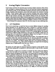
Frequency analysis structure An alternative to the time-interleaved structure is one that uses a bank of ADCs
in parallel to operate on separate frequency bands in what is referred to as a frequency analysis structure. The range of input frequencies is broken into a set of subband signals for analysis. A block diagram of the basic structure appears in Figure 1.2. All the ADCs in the structure are identical devices that operate on different subband signals. The filters Hk (z) are the analog decomposition filters, and the filters Gk (z) are the digital recombination filters. Because there is no modulation of signals to lower frequencies, the need for high-speed, high-precision sample-and-hold circuitry still exists [3]. Researchers
University of Maine MS Thesis Scott Saucier, December, 2002
3
H0 (z)
M
ADC
M
G0 (z)
H1 (z)
M
ADC
M
G1 (z)
H2 (z)
M
ADC
M
G2 (z)
HM −1 (z)
M
ADC
M
GM −1 (z)
y[n]
...
...
x(t)
analog
digital
Figure 1.2: M-channel frequency analysis ADC structure
University of Maine MS Thesis Scott Saucier, December, 2002
4
have argued that using identical quantizers in each channel offers a more flexible architecture.
1.1.3
Σ∆ ADCs used for channel quantizers Σ∆ ADCs are able to quantize signals with a high degree of resolution, provided
the signal energy is located at low frequencies compared to the sample rate. Using an integrating feedback loop, this converter applies a delay to the signal input and a noise shaping transfer function to the quantization noise. Signals that reside outside the narrow baseband region that is quantized with high resolution are pushed into the quantization noise that is shaped away from baseband. Using a one-bit quantizer and a one-bit digital-to-analog converter (DAC), Σ∆ ADCs are capable of achieving greater than 16-bits of resolution [4]. The Σ∆ ADC has been previously employed in a multiband scheme that used one lowpass converter and several bandpass devices [5]. A high degree of resolution was achieved across a bandwidth quantized by four devices. This work supports the idea that the Σ∆ ADC is a strong candidate for the quantizer used in each channel of the proposed structure due to the high resolution achieved by the converter. It is well suited to Very Large Scale Integration (VLSI) technology as it uses circuits that do not have to be well matched to produce high precision outputs.
1.2
Purpose of the research The purpose of this research is to formulate an architecture that makes use of
identical quantizers operating in parallel to efficiently perform wideband conversion. Each channel in the architecture contains identical hardware, so the cost of additional bandwidth is additional channels. The desired result is a structure that is able to recombine a number of smaller bandwidth signals into one with larger bandwidth. The recombined signal should have as little magnitude and phase distortion as possible across the total University of Maine MS Thesis Scott Saucier, December, 2002
5
recombined bandwidth, including where the edges of the smaller bands meet. The main focus of this thesis is the digital processing that allows the resolution of these parallel devices to be reliably extended to cover the first Nyquist band, which is half of the sample rate.
1.3
Thesis organization Chapter 2 looks at bandpass signals and the quantization of those signals. The
complex representation of bandpass signals is explained as well as the notation used throughout the remaining chapters to denote these signals. Different methods of sampling bandpass signals are discussed. Chapter 3 discusses the use of digital filter banks and their design. Multirate systems are discussed and an overview of the design of the proposed stucture is given. Chapter 4 gives an example of a filter bank designed specifically for the Σ∆ modulator designed for this project [1]. The performance of the recombination filter bank is examined. In support of this work, a monolithic frequency selective IQ Σ∆ modulator was designed and fabricated in a 0.5 µm CMOS process from AMI Semiconductor. This device is the prototype for the lowpass Σ∆ ADC unit used to quantize each band that is recombined digitally. Chapter 5 briefly examines the IC fabricated specifically for the architecture described in this thesis. The methods and results of the testing of the fabricated device are explained. Chapter 6 draws conclusions about the work presented in this thesis, and proposes ideas for future work.
University of Maine MS Thesis Scott Saucier, December, 2002
6
CHAPTER 2 BANDPASS SIGNALS This chapter provides an overview of bandpass signal quantization. The complex representation of bandpass signals is discussed in order to develop notation for later chapters and to provide insight on how bandpass signals are quantized. Different methods of sampling bandpass signals are discussed, and finally an outline of the proposed wideband ADC architecture is given.
2.1
Complex representation of bandpass signals A frequency spectrum Xc (F ) of a real, continuous time bandpass signal, xc (t),
is illustrated in Figure 2.1. A real signal with energy centered at frequency Fo also has energy at the conjugate frequency, −Fo . According to the Nyquist sampling theorem, a signal must be sampled at a rate that is at least twice the maximum frequency of the signal in order to quantize the signal without losing any information [6]. For a signal centered at frequency Fo with bandwidth B, the sample rate must be B Fs ≥ 2 Fo + , 2 �
�
(2.1)
Xc (F)
B
B
F -F o
F o
Figure 2.1: Frequency spectrum of a real bandpass signal
University of Maine MS Thesis Scott Saucier, December, 2002
7
which may be difficult to acheive for large Fo or B. All of the information needed to accurately represent xc (t) is contained in the positive frequencies centered at Fo , while the information contained in the negative frequencies centered at −Fo is a conjugate copy of that information. Since there is no need to retain both halves of the signal spectrum, one half of the energy shown (centered at either Fo or −Fo ) is enough to represent the signal, and the remaining half is redundant and can be ignored. Translation of the spectrum to the origin and lowpass filtering allows xc (t) to be represented at a much lower sampling rate. The highest frequency of interest is now B2 , and the sampling rate must be at least twice this amount or B Fs ≥ 2 2 �
�
= B.
(2.2)
This rate is usually considerably lower than the previous sampling rate and allows for more efficient processing of the signal. The corresponding lowpass signal, denoted x˜c (t), is given by x˜c (t) = L.P.P.{xc (t)e−j2πFo t }
(2.3)
where x˜c (t) is the “lowpass part” of the translated signal. The signal x˜c (t) is complex valued and is generated by lowpass filtering a complex modulated signal.
2.1.1
Complex modulation Translation of the frequency spectrum in the manner described above is acheived
by complex modulation (also known as vector modulation). Euler’s identity below gives the relations that are used to generate the translated signal. ejθ + e−jθ 2 jθ e − e−jθ sin(θ) = 2j
cos(θ) =
University of Maine MS Thesis Scott Saucier, December, 2002
8
(2.4)
Combining the cosine and sine waves allows separation of the complex exponential terms in (2.4). This separates the signal into its in-phase and quadrature parts, so named because the two terms have a 90 degree phase difference and thus are in quadrature with respect to each other. Either exponential term can be extracted using a combination of cosine and sine wave signals:
cos(2πFc t) + j sin(2πFc t) = ej2πFc t cos(2πFc t) − j sin(2πfc t) = e−j2πFc t .
(2.5)
Modulation of xc (t) with either of the complex sums shown in (2.5) yields a shift of the entire spectrum of xc (t) in just one direction because only one of the complex exponential terms are present in the modulation. This method eliminates the possibility of aliasing terms onto each other and allows the bandpass signal centered at Fo to be mixed all the way down to the origin. The concept of complex modulation using the separated exponentials is illustrated in Figure 2.2. The frequency spectrum Xc (F ) appears in Figure 2.2a. The complex exponential that modulates xc (t) has energy only at the frequency −Fc and none at the conjugate frequency Fc as shown in Figure 2.2b. When the two spectrums are convolved, as shown in Figure 2.2c, the resulting signal is complex valued in the time domain since the resulting spectrum is no longer symmetrical about the origin. The spectrum Xc (F ) has been shifted in only one direction, towards F = −∞, using the second complex sum from (2.5). (Note that using the first complex sum would simply result in the output spectrum shifted in the opposite direction, towards F = +∞.) The lowpass signal x˜c (t) is generated from a translated version of the sequence xc (t) using complex modulation by allowing Fc = Fo . As a result x˜c (t) is usually complex-valued when xc (t) is real. After the translation x˜c (t) is created by lowpass
University of Maine MS Thesis Scott Saucier, December, 2002
9
Xc (F ) A F −Fo
Fo
(a)
F{e−j2πFc t } = δ(F + Fc )
1
F −Fc
(b)
F{xc (t)e−j2πFc t } = Xc (F + Fc ) A F −Fc −Fo
−Fc + Fo
(c)
Figure 2.2: Complex IQ modulation
X c (F+Fo ) lowpass filter
B
~ X c (F)
F -2F c = -2F o
Figure 2.3: Lowpass representation of Xc (f )
University of Maine MS Thesis Scott Saucier, December, 2002
10
filtering the portion of Xc (F ) that now resides at the origin with bandwidth B as shown in Figure 2.3.
2.1.2 Properties of bandpass representations It can be shown that the original sequence, xc (t), can be recovered by translating x˜c (t) back to Fo and taking the real part of that complex-valued signal
xc (t) = 2Re{˜ xc (t)ej2πFc t }.
(2.6)
The signal given in (2.6) can be interpreted as
xc (t) = 2|˜ xc (t)| cos(2πFc t + 6 x˜c (t))
(2.7)
where 2|˜ xc (t)| is the envelope of the bandpass representation of xc (t) and 6 x˜c (t) is its phase. The reduced bandwidth of the complex representation makes it attractive for quantizers that sample bandpass signals to produce samples of x˜c (t) rather than xc (t). The sampled version of x˜c (t) is found by evaluating the signal at discrete points in time
x˜[n] = x˜c (nTs ) = L.P.P.{xc (nTs )e−j2πfo n }
(2.8)
where 1 Fs Fo = . Fs
Ts = fo
University of Maine MS Thesis Scott Saucier, December, 2002
11
(2.9)
n bits
xc (t)
Lowpass filter
e−j2πFo t
x˜c (t) ADC
x˜[n]
Fs
Figure 2.4: Sampling of bandpass signals
The structure shown in Figure 2.4 illustrates a bandpass sampling system as described above. The mixer and lowpass filter generate the signal x˜c (t) and the quantizer samples the lowpass signal to produce x˜[n]. Unfortunately x˜[n] cannot be created in this manner because ADCs cannot distiguish between real and complex waveforms and are incapable of sampling complex signals by themselves. The following section discusses methods used to sample a bandpass signal using the complex respresentation of that signal.
2.2
Bandpass sampling schemes Sampling bandpass signals requires a different approach than lowpass signals
due to the frequency of the bandpass signal. Signals at frequencies much higher than the sampling rate of the converter may need to be sampled, which can be complicated. Several techniques for sampling high frequency bandpass signals are now discussed.
2.2.1
IQ ADC structure A fairly common bandpass sampling structure is given in Figure 2.5. It consists
of an “in-phase” channel and a “quadrature” channel each feeding an ADC. The modulation by cosine and sine waves generates the terms for the complex modulation that shifts the spectrum down to the origin as explained in Section 2.1.1. The in-phase channel
University of Maine MS Thesis Scott Saucier, December, 2002
12
n bits
In−Phase
Lowpass filter
Re(˜ x[n])
ADC
xc (t) cos(2πFo t) n bits Lowpass filter
ADC
−Im(˜ x[n])
Quadrature
sin(2πFo t) Figure 2.5: Bandpass ADC IQ Structure
contains all the real bits of the output, while the quadrature channel contains all the imaginary bits. The complex signal can be obtained by adding the real portion with a phase-shifted version of the imaginary portion.
x˜[n] = Re(˜ x[n]) + jIm(˜ x[n])
(2.10)
Matching between the in-phase and quadrature channels is of great importance, as deviation from 90 degrees in the difference between the two channels can result in unwanted image frequencies. Gain mismatch between the two local oscillators can cause large tones at DC and
fs 2
that may couple with the input signal and induce unwanted
image frequencies. Analysis of both problems has been previously investigated [7]. These problems can arise as the result of analog circuitry imperfections in implementations of the in-phase and quadrature mixers.
2.2.2
Subsampling IQ structure One solution to reduce the sensitivity of demodulation to analog modulators in
the IQ structure is to perform the multiplication in the digital domain after sampling.
University of Maine MS Thesis Scott Saucier, December, 2002
13
n bits
In−Phase
Re(˜ x[n])
ADC
xc (t) cos
�
n bits
πn 2
�
−Im(˜ x[n])
ADC Quadrature
sin Figure 2.6:
Fs 4
�
πn 2
�
subsampling ADC IQ structure
This presents a problem when sampling high frequency signals, as the data rate must be increased accordingly. This technique, illustrated in Figure 2.6, makes use of subsampling in order to represent the bandpass signal at a lower frequency. When an analog signal is sampled, it is in effect multiplied by a sequence of delta functions, which causes the frequency spectrum of the sampled signal to be repeated at a period equal to the sample rate, Fs . A signal with energy at a frequency that is an integer multiple of Fs will therefore show energy at DC when sampled. By subsampling the bandpass signal, it can be quantized by a converter operating at a data rate much slower than the maximum frequency of interest in the signal. The technique of subsampling is used to perform most of the frequency translation on the bandpass signal, as mixing it all the way down to baseband would cause aliasing of the signal. Once the signal has been quantized, complex modulation is used to mix the signal down to DC as in the IQ structure. As described below, a popular choice is to select the sample rate so that the bandpass signal is aliased onto a bandwidth centered at
Fs . 4
At this point complex modulation is performed in the digital domain, which can
be done more reliably than with analog multipliers. The signal needs to be translated by Fs 4
1
which corresponds to multiplying the sequence by the complex exponential e−j2π( 4 )n
University of Maine MS Thesis Scott Saucier, December, 2002
14
n bits
xc (t)
x˜[n] ADC
3
e−j2π( 4 )n Figure 2.7:
3Fs 4
subsampling ADC IQ structure
which can be accomplished by using cosine and sine modulation in each channel: π π π cos n − j sin n = e−j 2 n . 2 2
�
The frequency
Fs 4
�
�
�
(2.11)
is chosen because the modulating signals are easily generated. The
signals are simply a stream of three values as shown below. π cos n = 1, 0, −1, 0, 1, 0, −1, 0, . . . �2 � π n = 0, 1, 0, −1, 0, 1, 0, −1, . . . sin 2 �
�
(2.12)
The use of ones and zeros eliminates the need to store any filter coefficients in memory. Due to the non-overlapping nature of the cosine and sine wave streams in (2.12), they can be combined into one digital stream consisting of 3
e−j2π( 4 )n = 1, j, −1, −j, 1, j, −1, −j, . . .
By sampling the bandpass signal so that it is centered at
3Fs , 4
(2.13)
only one channel is needed
because the complex modulation is performed digitally. One quantizer can produce the samples at a reduced rate using half as much hardware as needed for the architecture. The simplified structure appears in Figure 2.7.
University of Maine MS Thesis Scott Saucier, December, 2002
15
Fs 4
subsampling
At this point there are a few issues that should be considered using this toplogy in a multimode receiver. The input of the structure requires filtering to insure that nothing in any of the lower bands aliases into the signal during sampling. This filter is normally bandpass and attenuates everything but the desired signal band, which may be difficult at higher frequencies. For converting many bands, each ADC must operate at a different data rate, meaning the converters may not be the same in each channel.
2.2.3
Σ∆ bandpass sampling Bandpass versions of the Σ∆ converter have been developed that can quantize
a bandpass signal with high resolution, as it shapes quantization noise away from a particular center frequency. These converters acheive a bandwidth of high resolution that is limited to a small fraction of the sample rate, similar to that of the lowpass converter [8]. Σ∆ converters use low complexity circuits easily realized in VLSI technology to quantize signals with a high degree of resolution. They operate by sampling a signal at a rate that is many times higher than the bandwidth of the signal, which makes it an oversampled converter. An integrating feedback loop is used to average the samples taken by a one-bit quantizer to provide appropriate noise shaping in order to obtain a high resolution output. The oversampling spreads quantization error over a larger range of frequencies than critically sampled converters, and the integration and feedback push noise away from DC in what is called “noise shaping.” By altering the loop transfer function of a lowpass Σ∆ converter, a quantizer that provides noise shaping at a frequency other than DC can be constructed. These bandpass Σ∆ converters provide high resolution for a band of frequencies that is much smaller than the data rate.
University of Maine MS Thesis Scott Saucier, December, 2002
16
X(f) k=4
k=5
f= f 4
f 5
1 ___ 2
F Fs
Figure 2.8: Spectrum division for subband quantization
2.2.4
Σ∆ IQ structure The particular architecture implemented in this thesis uses Σ∆ ADCs in an IQ
structure. Different parts of the signal are modulated down to baseband where they are quantized by the ADCs in the in-phase and quadrature channels. The output of the structure is the complex representation of a bandpass signal quantized with the resolution of the Σ∆ converter. This structure can only quantize narrow bandwidth signals, much like the bandpass Σ∆. The frequency band that this structure operates on is variable, unlike the bandpass unit which operates on a fixed center frequency. Work done in [1] shows that the mixers in Figure 2.5 can be implemented in the front-end of a switched-capacitor Σ∆ ADC as will be explained in Chapter 5.
2.3
Proposed structure In order to quantize a signal with wide bandwidth, it is necessary to use multiple
ADCs running in parallel to quantize the signal. This system follows the frequency analysis approach to wideband quantization by dividing the input frequency range into a number of bands. The spectrum can be divided into M bands, each with bandwidth
University of Maine MS Thesis Scott Saucier, December, 2002
17
equal to
Fs . M
The band centers are given by
Fk =
where only the first
M 2
Fs k M
k = 0, 1, 2, ...
M −1 2
(2.14)
bands are converted due to the fact that the second Nyquist band
contains redundant information once the signal has been sampled. The division of the frequency spectrum is illustrated in Figure 2.8, where the spectrum of the quantized signal, x[n], has energy located in two different bands. Each band is processed by a separate channel containing the bandpass sampling modules. In each sampling module, the signal is demodulated in order to allow the quantizer in that channel to operate on a lowpass signal. The same type of converter can therefore be used to quantize different parts of the signal while operating at the same sample rate. The Σ∆ IQ ADC structure is employed to sample each bandpass section of the full signal. This method requires two ADC devices per channel for creating the in-phase and quadrature samples. The channels should be divided such that each channel is no larger than the bandwidth of the lowpass Σ∆ ADC which, due to the noise shaping, is normally considered to be BΣ∆ =
1 2OSR
(2.15)
where OSR is the over-sampling rate of the converter. The obvious choice for the channel width is to set the number of channels, M , equal to the over-sampling rate, meaning that the ADC conversion bandwidth and the channel bandwidth are the same. The filtering in each channel provides a means for selecting each bandpass part of the signal that will be recombined. It also serves to prevent aliasing of the signal when the signal is decimated. The most important consideration in the design of the filter banks is that the pieces of the original signal are recombined without causing any distortion at the edges of the bands. Adjacent signal bands must be filtered such that the edges add to reconstruct the information properly.
University of Maine MS Thesis Scott Saucier, December, 2002
18
Sampling module
xc (t)
frequency control
ω4 Recombination block
Sampling module
frequency control
xˆ4 [n]
y˜4:5 [n]
xˆ5 [n]
ω5
Figure 2.9: Recombination of 2 bands with proposed architecture
Figure 2.9 shows two channels of the M -channel structure. The signals xˆ4 [n] and xˆ5 [n] are decimated versions of the complex subband signals x˜4 [n] and x˜5 [n], respectively. The sampling module operates on a particular bandwidth of the signal centered at ωk in order to produce samples of x˜k [n]. The sampling module translates the signal band to baseband before quantization, and then decimates it in preparation for the recombination block. The signal y˜k:k+1 [n] is the recombined output of channels k through k + 1, where the subscript k : k + 1 is used to denote the channels that the recombined output spans. The signal y˜4:5 [n] can then be recombined with the signal y˜6:7 [n] from the adjacent recombination block in order to create the signal y˜4:7 [n] as shown in Figure 2.10. These blocks are simply cascaded in a tree structure to recombine additional bands.
University of Maine MS Thesis Scott Saucier, December, 2002
19
Sampling module
xˆ4 [n]
ω4
frequency control
Recombination block
Sampling module
xc (t)
y˜4:5 [n]
xˆ5 [n]
ω5
frequency control
Recombination block
Sampling module
xˆ6 [n]
ω6
frequency control
Recombination block
Sampling module
frequency control
y˜6:7 [n]
xˆ7 [n]
ω7
Figure 2.10: Recombination of 4 bands with proposed architecture
University of Maine MS Thesis Scott Saucier, December, 2002
20
y˜4:7 [n]
CHAPTER 3 FILTERING This chapter discusses digital filter banks and their applications in digital signal processing. A few different architectures are discussed, and important design aspects for a filter bank that performs the recombination for this application are given.
3.1
Digital filter banks Filter banks are important tools in digital signal processing that allow signals
to be separated into their smaller parts for simpler processing, often at a reduced data rate. A digital filter bank normally consists of a set of bandpass filters processing a common input signal or feeding a summed output. The bandpass filters usually pass non-overlapping signal bands. Filter banks are primarily broken into two catagories, which are analysis filter banks and synthesis filter banks. An analysis filter bank, shown in Figure 3.1a, takes one signal and filters it into several smaller bandwidth signals. Figure 3.1b shows a synthesis filter bank which performs the opposite function of combining a set of subband signals into one. Usually the emphasis in the design of a filter bank is on the quality of the separation or recombination. A system which does not distort the magnitude of the signal is said to be “magnitude preserving.” Such a system may scale the amplitude of the input signal. Most systems apply a sample delay to the input signal, as a finite amount of time is required to process the signal. A system that does not produce phase distortion or add a linear term to the phase of the signal is called “phase preserving.” A system that preserves both the magnitude and phase characteristics of the input signal is said to “perfectly reconstruct” the input signal. A perfect reconstruction system has a transfer function that resembles H(z) = az −d University of Maine MS Thesis Scott Saucier, December, 2002
21
(3.1)
H0 (z)
H1 (z) x[n]
vˆ0 [n]
v1 [n]
vˆ1 [n]
v2 [n]
vˆ2 [n]
G0 (z)
G1 (z) y[n] G2 (z)
...
...
H2 (z)
v0 [n]
HM −1 (z)
vˆM −1 [n]
vM −1 [n]
GM −1 (z)
(a)
(b)
Figure 3.1: (a) Analysis and (b) synthesis digital filter banks
where a is an amplitude scaling factor and d is an integer sample delay. The output of such a system is a scaled, delayed version of the input.
3.1.1 Uniform DFT filter banks Uniform DFT filter banks are constructed from a single lowpass prototype filter with real coefficients. The frequency response of the prototype filter is then translated in frequency to M uniformly spaced points across the frequency spectrum from DC (k = 0) to just below fs (k = M − 1). This is accomplished through complex modulation using the exponential 2π
kn e−j M kn = WM
(3.2)
where the commonly used notation 2π
Wλ = e−j λ
University of Maine MS Thesis Scott Saucier, December, 2002
22
(3.3)
v0 [n]
u0 [n]
...
2
H0 (z)
vˆ0 [n]
2
G0 (z)
x[n]
y[n] v1 [n]
u1 [n]
...
2
H1 (z)
vˆ1 [n]
2
G1 (z)
Figure 3.2: 2 channel QMF bank
has been used. The resulting filters (other than k = 0) all have complex coefficients and equal passband widths of
Fs . M
The input signal is then processed by these filters in
parallel which disects the signal into M bands for analysis. These filters are easily designed and implemented, since only one filter must be designed. This filter is a lowpass filter with bandwidth
Fs . 2M
In a variation of the uniform DFT filter bank, the same lowpass prototype filter is again designed. Instead of translating the frequency characteristic of the filter to select different bands, the input signal is translated so that the band of interest for each channel falls in the passband of the lowpass filter. The analysis filter bank consists of M copies (where M is the number of channels) of the lowpass prototype filter and the complex mixers that proceed the filters, each using a different local oscillator frequency 2πFk Fs 2πk = M
ωk =
k = 0, 1, 2, . . . M − 1.
(3.4)
The synthesis filter bank for this architecture also requires complex mixers in order to shift the pieces of the input signal back to their original postitions.
University of Maine MS Thesis Scott Saucier, December, 2002
23
3.1.2
Quadrature mirror filter banks A 2 channel quadrature mirror filter (QMF) bank, shown in Figure 3.2, is an
example of a multirate system [6]. The signal is processed at different rates throughout the system in order to acheive more efficient processing. This family of filter banks is so named because of the frequency response of the filters that comprise them. For the most basic two-channel version, the filters are symmetric about the quadrature frequency of ω = π2 . In the analysis filter bank, the input signal spectrum is divided in half, with the lower frequencies and the upper frequencies processed by separate channels. Because each channel only handles half of the input spectrum, the data can be coded at half the input sample rate. At this point the signals are either transmitted or further processed. When signals are received at the synthesis filter bank, the goal is to recombine data from the two channels to reconstruct the original signal. The sample rate is doubled in both channels before interpolation filters select portions of each channel for recombination. These filters must prepare the two halves of the spectrum to be recombined at the orignal sample rate. The equations that guide the design of the QMF bank are easily obtained through z-transform analysis of the signals at various points in the channels [6]. For the purpose of this analysis it is assumed that the signal does not undergo any processing between the analysis and synthesis banks. The signal is first filtered into a highpass and a lowpass signal in each channel Vk (z) = Hk (z)X(z)
(3.5)
where k is either 0 or 1 to designate the channel that passes DC or high frequency respectively. The signal is now divided between the two channels, with each channel processing half of the original signal. In order to achieve more efficient coding, the signals are decimated by a factor of 2. The down-sampling relation for decimation by a
University of Maine MS Thesis Scott Saucier, December, 2002
24
factor L in the z-domain is X 1 L−1 XD (z) = X(z 1/L WL−l ). L l=0
(3.6)
The downsampled signal in one channel is then found to be 1 [Vk (z 1/2 ) + Vk (−z 1/2 )] 2 1 = [Hk (z 1/2 )X(z 1/2 ) + Hk (−z 1/2 )X(−z 1/2 )]. 2
Uk (z) =
(3.7)
The downsampling introduces a certain amount of aliasing of the signals in each channel depending on the filters H0 (z) and H1 (z). This aliasing makes simple recombination of the signals difficult, and the filters G0 (z) and G1 (z) must be designed to cancel out the aliasing terms upon recombination. The upsampling relation for interpolation by a factor L is given by XU (z) = X(z L ).
(3.8)
After the sample rate is doubled in the synthesis bank, the signals are given by
Vˆk (z) = Uk (z 2 ) =
(3.9)
1 [Hk (z)X(z) + Hk (−z)Xk (−z)]. 2
The recombined signal Y (z) is the sum of the filtered outputs from both channels
Y (z) = Vˆ0 (z) + Vˆ1 (z) =
1 [H0 (z)G0 (z) + H1 (z)G1 (z)]X(z) 2 1 + [H0 (−z)G0 (z) + H1 (−z)G1 (z)]X(−z). 2
University of Maine MS Thesis Scott Saucier, December, 2002
25
(3.10)
The relation in (3.10) is separated into two terms
Y (z) = T (z)X(z) + A(z)X(−z)
(3.11)
where the first term is the desired output of the system, and the second term is unwanted distortion. The signal X(z) occupies the entire bandwidth, and the addition of X(−z) represents aliased information in the signal. The goal is to design the filters Hk (z) and Gk (z) such that A(z) = 0.
(3.12)
An alias-free realization of the two-channel QMF structure can be designed by choosing
H1 (z) = H0 (−z) G0 (z) = H0 (z) G1 (z) = −H1 (z) = −H0 (−z)
(3.13)
which meets the requirement of (3.12). The solution is then reduced to designing the filters H0 (z) and H1 (z) such that
|H0 (z)|2 + |H1 (z)|2 = 1.
(3.14)
Filters H0 (z) and H1 (z) are said to be power complimentary when (3.14) is satisfied. Filter banks using linear phase filters, with responses as given in (3.14), are perfect reconstruction filter banks [6]. The degree to which the output of the QMF bank resembles the input determines the recombination performance. Much emphasis has been placed on the design of linear phase perfect reconstruction filter banks (LPPRFBs). Straightforward analysis is only
University of Maine MS Thesis Scott Saucier, December, 2002
26
able to produce a trivial case for which linear phase filters can be designed to satisfy the perfect reconstruction requirements. In order to find more solutions, one of the requirements is relaxed and optimization routines can find close solutions. Usually the magnitude preserving requirement of (3.14) is relaxed and linear phase filters are used as in [9]. Filter coefficients are then iteratively adjusted to provide as little distortion at the band edges as possible. The theory behind QMF banks has been extended beyond the two-channel case to include M -channel structures. These are well suited to the recombination of several bands of digitized signals. A similar approach to the M -channel case is taken in the design of the proposed structure.
3.2
Multirate filter bank for signal reconstruction The filter bank structure in this design is modeled after the QMF bank structure
given in Section 3.1.2. Each channel is decimated to allow more efficient processing of the signal in later stages, and the filter design is governed by the transfer function of the recombined signal. The major difference between this design and the QMF bank is that the QMF bank is almost always optimized for reassembling a predetermined number of channels (which is usually the same number of channels that were separated in the system). The degree to which the signal is reconstructed depends on the frequency responses of all of the filters in the bank. The QMF bank does not perform as well if any of the channels are left out of the recombination. The design proposed in Section 2.3 allows the user to determine the number of recombined channels based on the needs of the receiver. The only limit to the number of recombined channels is that it needs to be a multiple of two, as the system recombines two adjacent bands at every stage regardless of the size of the bands. These bands double in size at every stage, so the system has a tree-like structure.
University of Maine MS Thesis Scott Saucier, December, 2002
27
HD (z)
x[n]
x ˆk [n]
x ˜k [n]
sk [n]
uk [n]
D
2
vk [n]
ak [n]
HI (z)
e−j ( 2M )n πD
e−jωk n
HD (z)
e−jωk+1 n
D
2
HI (z)
x ˆk+1 [n]
sampling modules
y˜k:k+1 [n]
ak+1 [n] πD j ( 2M )n
e
recombination block
Figure 3.3: Channel recombination for a 2-channel system
The basic 2-channel structure that allows digital recombination of a wideband signal from its subband quantized parts is shown in Figure 3.3. The structure is the realization of that in Figure 2.9 used to recombine two adjacent channels. Additional channels are recombined through repeated stages of the recombination block. The demodulation and decimation at the front of the channel prepare the signal for the recombination stage. This implementation uses linear phase filters to preserve the phase information of the signal. Magnitude distortion is minimized by matching the transition edges of the filters of adjacent channels together, so the only distortion comes from passband ripple.
3.2.1
Band demodulation The demodulation step selects the particular band that will be processed by
each channel. As discussed in Section 2.1.1, complex modulation is used to obtain the lowpass complex representation of the subband signal. The entire signal is processed through in-phase and quadrature channels where it is multiplied by the complex exponential from (3.2) with the superscript k indicating which band the channel will operate on as University of Maine MS Thesis Scott Saucier, December, 2002
28
x[n]
H2D (z)
D 2
y[n]
−jωk+ 1 n
e
2
Figure 3.4: Equivalent system of Figure 3.3
in (2.14). Each channel needs two quantizers and two mixers to create the samples, although it should be noted that the two channels for in-phase and quadrature signal generation are different than the channels that recombine two adjacent parts of the signal. The best way to implement the demodulation step is to perform the multiplication after the signal has been digitized. “Pre-sampling” the signal using a sampleand-hold (S/H) circuit, with different capacitor values, allows a digital multiplication of the signal before it reaches the quantizer. Performing the frequency translation inside the ADC may also be an option, depending on the converter topology chosen. In Figure 3.3 it is assumed that the signal has been quantized before the filter bank is applied for the purposes of the following analysis.
3.2.2
Filtering and sample rate conversion The process of filtering the bandpass signals in the system is performed at several
different sample rates. The filters HD (z) and HI (z) serve two purposes. They prevent aliasing during decimation and filter out redundant information after interpolation. They must be designed so that neighboring bands can be recombined without causing any distortion at the band edges. If the system is able to recombine two channels without distorting either subband signal, then the composite system should be equivalent to the
University of Maine MS Thesis Scott Saucier, December, 2002
29
system of Figure 3.4, where the filter H2D (z) has a bandwidth that is twice that of filter HD (z). The analysis of the two channel recombination filter bank follows very closely to that of the QMF bank. The intermediate signals along the path of each channel in Figure 3.3 are now examined. For a system consisting of M channels, the sampled bandwidth of each subband signal xˆk [n] is
1 . M
The shifted version of x[n], denoted
sk [n], has z-transform
Sk (z) = X(zejωk ) −k = X(zWM )
(3.15)
where (3.4) has been substituted for ωk . The signal x˜k [n] is the complex representation of the subband signal to be recombined, which is created by the methods discussed in Section 2.1. This signal is simply a filtered version of sk [n], where the filter hD [n] is designed to eliminate any terms that may alias onto the desired band after further processing. The decimation by a factor D allows the desired signal to fill most of the new sampling bandwidth which makes subsequent processing much easier in terms of filter coefficients and resolution. However, the down-sampling might also corrupt the signal if the filter hD [n] is not designed correctly. Decimation stretches the frequency axis but, due to the nature of the sampled signal, its frequency spectrum is always periodic with period f = 1. The lowpass filter HD (z) must therefore pass the signal in the range |f | ≤
1 2M
and attenuate signals past the frequency f =
1 1 − 2M . D
The processed bandpass
signal xˆk [n] appears in the z-domain as Xˆk (z) = =
University of Maine MS Thesis Scott Saucier, December, 2002
X 1 D−1 ˜ k (z 1/D W −i ) X D D i=0 X 1 D−1 −k HD (z 1/D WD−i )X(z 1/D WD−i WM ). D i=0
30
(3.16)
H (f) D
1 δ f 1 __ M
Figure 3.5: Decimation filter HD (z) frequency response
At this point it is important to note the value of the decimation rate D in relation to the number of channels M . It is allowable to have D ≤ M , since the data in the channel will be preserved as long as the bandwidth after decimation and filtering is ≤
1 . M
For D > M the narrow band signal will be subject to aliasing, which will distort
the signal in a manner that cannot be reversed. For the following discussion on different decimation rates it is assumed that the frequency response of the filter HD (z) is as shown in Figure 3.5 where the finite transition bandwidth of the filter, denoted δ, is defined.
Case 1 - Maximally decimated filter bank The filter bank with D = M is called maximally decimated, which means that the final decimated bandwidth is as wide as each channel, with no spare room at the edges. This can be a problem when the decimation filter has a finite transition bandwidth. The original spectrum of the sampled signal X(f ) appears in Figure 3.6(a), where the frequency bands of interest for k = 4 and k = 5 are noted. The adjacent ˆ 4 (z) and X ˆ 5 (z), are targeted for recombisignals for these particular values of k, X nation. Due to the filter transfer function, HD (z), only a small band of the original signal is passed to the down-sampler in each channel. The filter HI (z) also has a lowpass transfer function, so the i = 0 term in (3.16), which is centered at DC, is the term that the
University of Maine MS Thesis Scott Saucier, December, 2002
31
X(f) k=4
k=5 D=M
f 1 __ 2 (a) Frequency spectrum of wideband signal X 1 D−1 −(4+i) Xˆ4 (z) = HD (z 1/D WD−i )X(z 1/D WD ) D i=0
i=0
i=1
��� ���
������ ��
1 __ 2
��������� ������
f
1 __ 2
1 __ 2
f
1 __ 2
��������� ������ ��������������� ������ ���� 1 __ 2
i=D-1
f 1 __ 2
ˆ 4 (z) (b) Potential aliasing terms of X X 1 D−1 −(5+i) ˆ X5 (z) = HD (z 1/D WD−i )X(z 1/D WD ) D i=0
i=0
��� ��� �
1 __ 2
i=1
������ ��
f
1 __ 2
1 __ 2
��������� ������ ��������������� �����
i=D-1
f
1 __ 2
��������� ������ ����� 1 __ 2
f 1 __ 2
ˆ 5 (z) (c) Potential aliasing terms of X
Figure 3.6: Terms of concern for aliasing using decimation with D = M
University of Maine MS Thesis Scott Saucier, December, 2002
32
filter bank should preserve. When the decimated signal covers the entire first Nyquist band there may be some aliasing from the adjacent terms i = 1 and i = M − 1 in the ˆ 4 (z) and X ˆ 5 (z) are shown in Figures sum. The terms of interest in the summation for X 3.6(b) and 3.6(c), respectively. It can be seen that for the case where D = M there is aliasing at the band edges due to these adjacent terms, where shading has been used to illustrated the areas of overlap for each term. The residue from the adjacent terms that leaks onto the i = 0 term is caused by the finite transition bandwidth δ of the filter HD (z). This aliasing causes distortion that cannot be undone simply by interpolation and filtering. It is for this reason that this design focuses on finding solutions for filter banks that use D < M .
Case 2 - Relaxed decimation By relaxing the decimation rate compared to the number of channels, the amount of aliasing can be significantly reduced. Leaving space between each aliased term for the overlap of the transition bandwidth of the decimation filter HD (z) allows the interpolation filter HI (z) to eliminate all other terms other than desired signal. After these terms have been removed, the recombination depends on lining up the edges of signals that have been filtered by HD (z). The filter design problem then becomes finding a good design for HD (z). Figure 3.7 illustrates relaxed decimation by D =
M , 2
where the same parts of the
original wideband signal, shown again in Figure 3.7(a), are to be processed. The terms in Figure 3.7(b) and 3.7(c) are still centered at the same frequencies, but now they are half as wide as before. This leaves space between the three terms, and there is no overlap between terms. The stopband attenuation of filter HD (z) must be large enough so that any aliased terms will be negligable. The case for D =
M 2
is the largest decimation rate
that can be used without causing any aliasing of the desired term.
University of Maine MS Thesis Scott Saucier, December, 2002
33
X(f) k=4
k=5
M D= ___ 2
f 1 __ 2 (a) Frequency spectrum of wideband signal X −( 4 +i) 1 D−1 Xˆ4 (z) = HD (z 1/D WD−i )X(z 1/D WD 2 ) D i=0
i=0
i=D-1
i=1
f 1 __ 2
f
1 __ 2
1 __ 2
f 1
1
1 __ 2
ˆ 4 (z) (b) Potential aliasing terms of X X −( 5 +i) 1 D−1 Xˆ5 (z) = HD (z 1/D WD−i )X(z 1/D WD 2 ) D i=0
i=0
i=D-1
i=1
f 1 __ 2
1 __ 2
f 1 __ 2
1
f 1
1 __ 2
ˆ 5 (z) (c) Potential aliasing terms of X
Figure 3.7: Terms of concern for aliasing using decimation with D =
University of Maine MS Thesis Scott Saucier, December, 2002
34
M 2
By using a decimation rate D < M , a linear phase filter bank can be designed that eliminates any contribution to the signal by terms other than i = 0 in (3.16). For the purpose of the analysis, the signal xˆk [n] now appears as 1 −k Xˆk (z) = HD (z 1/D )X(z 1/D WM ) D
(3.17)
provided that D < M . The requirements for the filter HD (z) at this point are that it needs to pass signals in the range 0 ≤ f ≤
1 M
amount of attenuation to signals in the range
− 2δ , and that it needs to provide a large 1 M
+
δ 2
≤ f ≤
1 . 2
The transition band
requirements will be derived once the recombination stage has been discussed.
3.2.3
Recombination stage The recombination stage is designed to add together two adjacent bands of the
same bandwidth. As shown in Figure 3.3, the recombination begins with an interpolation step that increases the sample rate by a factor of two. This widens the sampled bandwidth to a size that is large enough to fit the signals from both channels. The signal uk [n] is an up-sampled version of the subband signal xˆk [n] given in the z-domain by Uk (z) = Xˆk (z 2 ) =
1 −k HD (z 2/D )X(z 2/D WM ). D
(3.18)
The interpolation produces another copy of the desired signal band in the sampled bandwidth, and the interpolation filter, HI (z), is included to remove that copy. The signal vk [n] is the lowpass filtered version of uk [n], meaning that vk [n] and the signal produced from the adjacent band, vk+1 [n], each contain the lowpass versions of the subband signals for the k and k + 1 bands. These signals are then complex modulated in different directions in order to construct the lowpass version of the signal bandwidth that
University of Maine MS Thesis Scott Saucier, December, 2002
35
is twice as large as that in a single channel. The size of the frequency translation depends on the down-sampling rate. The two channels should be shifted by half the width of the signal band after the interpolation filter, which for the maximally decimated case, would be f = 14 . For the case of relaxed decimation, this shift is scaled by the ratio of yielding a shift of f =
D . 4M
D , M
The signal ak [n] in the z-domain is found to be πD
Ak (z) = Vk (zej 2M n ) πD π π 1 −k HI (zej 2M )HD (z 2/D ej M )X(z 2/D ej M WM ) D 1 −(k+ 1 ) −D/4 −1/2 = HI (zWM )HD (z 2/D WM )X(z 2/D WM 2 ) D
=
(3.19)
and the signal ak+1 [n] in the opposite channel is given by
Ak+1 (z) =
1 −(k+ 1 ) D/4 1/2 HI (zWM )HD (z 2/D WM )X(z 2/D WM 2 ) D
(3.20)
where (3.3) has been substituted into the appropriate locations. The two signals ak [n] and ak+1 [n] are then summed, which gives the recombined two-channel output Y˜k:k+1 (z) = Ak (z) + Ak+1 (z) =
1 −D/4 −1/2 [HI (zWM )HD (z 2/D WM ) D D/4
1/2
−(k+ 12 )
+HI (zWM )HD (z 2/D WM )]X(z 2/D WM
).
(3.21)
The signal X(z 2/D ) has twice the bandwidth of the signal in each channel, and the k+ 12
modulation term WM
shows that it has been translated from a frequency that lies
between the two adjacent bands. If the decimation and interpolation filters, HD (z) and HI (z), are designed such that HI (z) passes all of the frequency selectivity of HD (z) (i.e. the cascading of HD (z) and HI (z) yields an equivalent filter HD (z)), then this system does approximate the equivalent system of Figure 3.4.
University of Maine MS Thesis Scott Saucier, December, 2002
36
3.2.4
Filter design Attention must now be turned to the design of the filters in the system. An
advantage to using this architecture is the fact that there are only two digital filters in the system, which means only two sets of coefficients need to be stored. This is an advantage over most other perfect reconstruction filter banks, which often use a different filter design for each channel. The most critical design will be for hD [n] because it determines the performance of the system at the band edges. The lowpass frequency response of HD (f ) is required to pass the band
−1 2M
≤ f ≤
1 2M
(before the sample
rate conversion) and stop everything else with a large amount of attenuation. Due to the fact that digital filters (or any filters, for that matter) cannot be designed to have zero transition bandwidth, it is assumed there is a finite transition bandwidth δ in the frequency response of hD [n] that needs to be preserved by hI [n] as shown in Figure 3.5. The interpolation filter therefore needs to have a passband edge which is above
1 2M
+ 2δ .
After decimation by a factor of D and upsampling by a factor of 2, the required passband for the design of the interpolation filter becomes |f | ≥
D 4M
+
δD . 4
The upsampling also
produces an undesired “copy” of the signal band centered at f = 21 . This copy must be eliminated by the interpolation filter. The requirements of the interpolation filter are that it must pass the desired term centered at f = 0 that covers the range of frequencies −D 4M
−
range
δD 4 1 2
≤f ≤
D − ( 4M +
D 4M δD ) 4
+
δD , 4
and reject the aliased term centered at f =
≤f ≤
1 2
D + ( 4M +
δD ). 4
1 2
covering the
Table 3.1 summarizes the passband and
stopband edge requirements for the filter hI [n]. The general case for decimation by D is given and the cases for D = M and D =
M 2
are evaluated for comparison. As stated
in Section 3.2.2, the aliased terms overlap the edges of the desired signal for the case of maximal decimation, which is shown again in the values in the table for the passband and stopband edges of hI [n]. The values for decimation by D =
M 2
show the spacing
between terms (provided that δM < 1) that eases the filter design. Figure 3.8 further
University of Maine MS Thesis Scott Saucier, December, 2002
37
decimation rate D (general)
passband |f | ≤
D 4M
+
stopband δD 4
1 2
D − ( 4M +
δD ) 4
≤f ≤
1 2
+
D 4M
D=M
|f | ≤
1 4
+
δM 4
1 4
−
δM 4
≤f ≤
3 4
+
δM 4
M 2
|f | ≤
1 8
+
δM 8
3 8
−
δM 8
≤f ≤
5 8
+
δM 8
D=
+
δD 4
Table 3.1: Requirements of the interpolation filter for different rates of decimation
HI (z) 1 HD (z) f 1 2 1 8
+
δD 4
3 8
−
1
δD 4
Figure 3.8: Requirements for interpolation filter HI (z) frequency response (for D =
University of Maine MS Thesis Scott Saucier, December, 2002
38
M ) 2
x[n]
y[n] H D (z)
D
(a) Single-stage decimation by D
x[n]
y[n] H A(z)
D
H B(z)
(b) Multistage filtering of HD (z)
x[n]
y[n] H D1 (z)
D1
H D2 (z)
D2
H B(z)
(c) Two stage decimation by D
Figure 3.9: Multi-stage decimation and filtering illustrates the filter requirements of hI [n] for the case D =
M , 2
where the upsampled
terms that have been filtered by hD [n] are also shown. The decimation filter hD [n] processes every channel with a lowpass response. Since it must be possible to recombine adjacent channels in the reconstruction, the filter hD [n] must have a symmetrical design. Due to the high decimation rate, designing filters with passbands that are small relative to the sampling frequency is difficult. Designing these filters with tight specifications in the transition band is even more difficult because the transition band is also small.
3.2.4.1
Multistage decimation The steps in the design process of the filter HD (z) are illustrated in Figure 3.9,
where the straightforward approach to decimation by D is shown in Figure 3.9(a). The filter design can be simplified if it can be done at a lower sampling rate where the passband and the transition band δ take up a larger part of the sampling bandwidth.
University of Maine MS Thesis Scott Saucier, December, 2002
39
By breaking the filter hD [n] into two separate filters with one filter each used to process the signal before and after decimation, the design becomes much easier. This method, shown in Figure 3.9(b), divides the responsibilities of the decimation filter between the two new filters, HA (z) and HB (z). The filter HA (z) that precedes the down-sampling is used to remove any signal components that may alias into the particular band of interest. This filter design focuses on the location of stopbands rather than the symmetric passband edges, which is not a difficult design if the decimation rate is fairly low. For higher decimation rates the act of down-sampling is often performed by cascading filter and decimation blocks, a technique that is illustrated in Figure 3.9(c). The filter HA (z) and the decimation by D has been split into two new stages composed of filters HD1 (z) and HD2 (z) and decimation by factors of D1 and D2 (where D1 D2 = D). The complexity of the filter in each stage is reduced by the following stage because the number of aliased bands that must be filtered out at each stage decreases as the number of stages increases. The spacing between these aliased bands therefore increases with the number of decimation stages, which also makes the designs for HD1 (z) and HD2 (z) easier [6]. The filter HB (z) at the end of the decimation stage in Figures 3.9(b) and 3.9(c) provides the symmetric edges for recombination. This filter is always implemented at the lowest sampling rate in the two-channel stage, which makes it a much simpler design than the original solution of using a single filter.
3.2.4.2
Half-band filters As previously stated, in order to recombine the signals from two neighboring
bands, the filter HD (z) should have symmetric edges. For a decimation rate of D =
M 2
the filtered signal xˆk [n] covers the range |f | ≤ 14 + δM . The filter HD (z) must then have 4 symmetric edges about the frequency f =
1 4
so that the two signals xˆk [n] and xˆk+1 [n]
will add together correctly at the band edges. The transition band
University of Maine MS Thesis Scott Saucier, December, 2002
40
δM 2
should extend
H2 (ejω ) 1 H2 ∗ (ej(π−ω) ) 1 2
ω ωP
ωS
π 2
π
Figure 3.10: Frequency response of a half-band filter
equally into the passband and stopband. The filter bank composed of the two filters −1/2
1/2
represented by the terms HD (z 2/D WM ) and HD (z 2/D WM
) from (3.21) should be
some form of complimentary filter bank. A delay-complimentary filter bank is classified as M −1 X
Hγ (z) = βz α
β 6= 0
(3.22)
γ=0
where the filters Hγ (z) compose the M -channel filter bank [6]. The filters of a delaycomplimentary bank add together to pass the entire sampled bandwidth. A set of filters called half-band filters meet the above requirements of being symmetric and complimentary. These filters are part of the class of Lth-band filters, which are characterized by having a zero at every Lth coefficient in its impulse response. The term at the origin is a constant, and these requirements are given in the standard equation for even order Lth band filters:
hL [nL] =
University of Maine MS Thesis Scott Saucier, December, 2002
α,
n = 0,
0,
otherwise.
41
(3.23)
Half-band filters are Lth band filters where L = 2 and α = 21 . Since every even indexed coefficient except for h2 [0] is zero, the polyphase decomposition of H2 (z) yields
H2 (z) =
1 + z −1 E1 (z 2 ) 2
(3.24)
where E1 (z) is the first polyphase component of H2 (z), and the polyphase components of an Lth band filter are found by ∞ X
Ek (z) =
hL [k + nL]z −n
0 ≤ k ≤ L − 1.
(3.25)
n=0
The relation given in (3.24) can be reduced to
H2 (z) + H2 (−z) = 1.
(3.26)
If h2 [n] has real coefficients, then H2 (−ejω ) = H2 ∗ (ej(π−ω) ), and (3.26) gives H2 (ejω ) + H2 ∗ (ej(π−ω) ) = 1.
(3.27)
This equality shows that the half-band filter exhibits symmetry about the quadrature frequency ω = 2π
� � 1 4
=
π 2
as shown in Figure 3.10. It also shows that the two filters in
(3.27) are complimentary. The passband and stopband edges are symmetric with respect to ω = π2 , meaning that ωp + ωs = π and ωs − ωp = δ. The filter also has equal passband and stopband ripple [6]. Half-band filters only pass the first half of the sampling bandwidth centered at f = 0. The half-band filter is used to set the final signal bandwidth for the channel as shown in Figure 3.7, where for the case D =
M , 2
the i = 0 term covers the range
|f | ≤ 41 , which corresponds to the passband of the half-band filter. The edges of two half-band filters operating on opposite halves of the spectrum add up to a constant across
University of Maine MS Thesis Scott Saucier, December, 2002
42
the transition band, as shown by (3.27). This property is desired of the filter HD (z), and since the last filter in Figure 3.9(c) sets the transition band characteristic, the filter HB (z) is chosen to be a half-band filter.
3.2.5
Signal delay The linear phase filters used in this design all impose different sample delays on
the signal as it moves through the system. As the signals are modulated in the recombination block, terms are generated that alter the phase of the signals. These terms are scale factors that must be corrected in order to assure that the entire system is linear phase and does not distort the group delay of the signal. A causal filter has linear phase if its impulse response is either symmetric or antisymmetric [6]. Filters that display symmetry can be represented in the form
H(z) = z −l HR (z)
(3.28)
where l respresents a unit sample delay and HR (z) is the real-valued amplitude response of the filter. For a filter of order N (either symmetric or antisymmetric) that has N + 1 coefficients, the value of l is given by
l=
N . 2
(3.29)
As linear phase filters, hD [n] and hI [n] can be decomposed as in (3.28) to yield HD (z) = z −l1 HDR (z) HI (z) = z −l2 HIR (z).
University of Maine MS Thesis Scott Saucier, December, 2002
43
(3.30)
The changes in the phase of the signal as it is processed by the system can be found by substituting (3.30) into (3.19) to find l1 −2l1 π 1 −l2 −j πl2 −(k+ 1 ) −1/2 z e 4 HIR (zej 4 )z D WM2 HDR (z 2/D WM )X(z 2/D WM 2 ) D 1 −(k+ 1 ) c −D/4 −1/2 = HIR (zWM )HDR (z 2/D WM )X(z 2/D WM 2 )z −dk:k+1 WMk:k+1 D
Ak (z) =
(3.31)
where the cofficients dk:k+1 and ck:k+1 are given by 2l1 + l2 D l1 l2 D = + . 2 4
dk:k+1 = ck:k+1
(3.32)
Similarly, the signal in the opposite channel is found using (3.20) to be
Ak+1 (z) =
1 −(k− 1 ) −c D/4 1/2 HIR (zWM )HDR (z 2/D WM )X(z 2/D WM 2 )z −dk:k+1 WM k:k+1 . D (3.33) c
The phase shift WMk:k+1 needs to be corrected in each stage in order to maintain a linear phase characteristic to give the phase corrected recombined output. The signal y˜k:k+1 [n] becomes −c c Y˜k:k+1 (z) = Ak (z)WM k:k+1 + Ak+1 (z)WMk:k+1 .
(3.34)
The delay term that is left, z −dk:k+1 , will produce phase shift terms in the next stage. All the recombination blocks are identical to that shown in Figure 3.3. For the second stage, the inputs y˜k:k+1 [n] and y˜k+2:k+3 [n] are recombined to give y˜k:k+3 [n]. The signal ak:k+1 [n] produced from the input y˜k:k+1 [n] is given by Ak:k+1 (z) = z −l2 e−j
University of Maine MS Thesis Scott Saucier, December, 2002
πl2 4
−D/4
HIR (zWM
44
π
)Y˜k:k+1 (z 2 ej 2 ).
(3.35)
stage 1 2 3 4
# bands 2 4 8 16
coefficient ck:k+1 ck:k+3 ck:k+7 ck:k+15
coefficient formula l1 + l24D 2 l1 + 3l24D = 2ck:k+1 + l24D 2l1 + 7l24D = 2ck:k+3 + l24D 4l1 + 15l42 D = 2ck:k+7 + l24D
factor ±c WM k:k+1 ±c WM k:k+3 ±c WM k:k+7 ±c WM k:k+15
Table 3.2: Phase shift factor coefficients for 4 stages of an M -channel system
Substitution of (3.31) through (3.34) into (3.35) yields new delay and phase shift terms
dk:k+3 =
4l1 + 3l2 D
= 2dk:k+1 + l2 ck:k+3 = l1 +
3l2 D 4
= 2ck:k+1 +
l2 D 4
(3.36)
where the old delay and phase shift coefficients have been doubled by the interpolation step, and an additional amount of delay and phase shift is put on the signal by the filter hI [n] in every recombination stage. The second stage output y˜k:k+3 [n] is found as in (3.34) using the new phase shift factors −c c Y˜k:k+3 (z) = Ak:k+1 (z)WM k:k+3 + Ak+2:k+3 (z)WMk:k+3 .
(3.37)
The generation of these phase shift correction factors is an iterative process through the system, and corrections must be made at the output of every stage. Factors for the first four stages of a system using decimation of D =
M 2
are given in Table 3.2. It should be
noted that factors generated from recombining the same number of bands are equal, for example ck:k+3 = ck+4:k+7 = ck+6:k+9 where all of the factors are generated from the recombination of 4 signal bands.
University of Maine MS Thesis Scott Saucier, December, 2002
45
(3.38)
x[n]
xˆk [n] HD1 (z)
D1
HD2 (z)
D2
HB (z)
e−jωk n Figure 3.11: Final channel decimation block design
3.3
Filter bank design summary The final design for the recombination filter bank includes all of the parts discussed
in Section 3.2. The design for the decimation and filtering in each channel prior to recombination appears in Figure 3.11. The decimation filter is implemented in two parts, where the first filter selects the proper frequency range to pass by eliminating any signals that may alias onto the desired signal during the decimation. This filter, along with the decimation block, is implemented in two stages composed of filters HD1 (z) and HD2 (z) and decimation by D1 and D2 . The two stage decimation makes filter design easier than a single stage decimation. The second part of the decimation filter, the halfband filter HB (z), sets the transition band of the filtering process so the band edges will line up when the signals are recombined. The final design for the recombination block is shown in Figure 3.12. The upsampling block and the interpolation filter HI (z) increase the sample rate by a factor of two. The signal in each channel is then modulated in oppostie directions to be recombined. The phase correction factors are applied after modulation in each channel with opposite signs on each exponential. The signals are then added together to complete the recombination step. Specific digital filter designs are given in the next chapter.
University of Maine MS Thesis Scott Saucier, December, 2002
46
xˆk [n] 2
c
WMk:k+1
HI (z)
y˜k:k+1 [n] πD −j 2M n
e xˆk+1 [n] 2
−ck:k+1
WM
HI (z)
πD
ej 2M n
Figure 3.12: Final recombination block design
University of Maine MS Thesis Scott Saucier, December, 2002
47
CHAPTER 4 ARCHITECTURE DESIGN This chapter shows the design of a recombination filter bank for use with Σ∆ ADCs. The specifications for the data converters that govern architecture design are discussed, and the decimation and interpolation filter designs are given. The recombination performance of the filter bank is examined through MATLAB simulation, and finally the architecture is simulated with Σ∆ sampling modules.
4.1
Channel ADCs This particular design uses Σ∆ ADCs to quantize the subband signal in each
channel. This allows each band of frequencies to be quantized with a high degree of resolution. The end result is that the noise-shaping effect of the Σ∆ ADC appears in each band across the first Nyquist Band.
4.1.1
Frequency selective IQ Σ∆ ADC The Σ∆ architecture simulated in this design example is modeled after the fre-
quency selective IQ Σ∆ ADC circuit designed and constructed in [1]. This device implements the modulators and ADCs all in one package. In-phase and quadrature channels are used to produce complex samples of the bandpass representation of the signal in each band. The prototype built in [1] used a fourth-order multistage noise shaping (MASH) architecture composed of two cascaded second-order loops in each channel, although for the purposes of this simulation, different order loops are used to model the ADC. The oversampling rate (OSR) is 32, and the modulators are configured to select one of 16 bands across the first Nyquist band for quantization.
University of Maine MS Thesis Scott Saucier, December, 2002
48
x[n]
y[n] H D1(z)
4
H D2(z)
4
H B (z)
Figure 4.1: Cascaded downsamplers to achieve decimation by 16
4.1.2
Division of channels Fs , so this sets The useable bandwidth of a Σ∆ ADC is normally given to be OSR
the bandwidth of each channel in the system. One IQ Σ∆ structure is used to quantize the information in each band. The bands are divided as shown in Figure 2.8, which illustrates the case for M = 16 where the first 8 channels are to be quantized and reconstructed. In order to model the hardware, this simulation has 32 channels, and the first 16 channels are to be recombined. Each subband signal has a bandwidth of B = and each band is centered at fk =
k M
for k = 0, 1, 2, ...15. Each channel prepares the
subband signal for recombination using a relaxed decimation of D =
4.2
1 , M
M 2
= 16.
Filter designs Linear phase filters are used in this design in order to preserve the group delay
of the input signal. The amplitude information is kept intact by designing the filters to provide enough attenuation to the signals outside the band of interest, as well as using a symmetrical design for the decimation filter so that adjacent band edges will add correctly.
4.2.1
Decimation filtering The filter designs hD [n] and hI [n] are critical to the performance of the system.
The passband ripple of both filters should be low so that the desired signal is not distorted, and the stopband attenuation should be high to prevent the aliasing of unwanted
University of Maine MS Thesis Scott Saucier, December, 2002
49
terms. For these reasons the filters are designed to have a maximum passband ripple of 0.1 dB and a minimum stopband attenuation of at least 100 dB. The design of the decimation filter hD [n] shows that a high OSR can make the filter design quite difficult. For OSR = 32, Figure 3.5 shows that the required filter has a lowpass characteristic with a passband edge frequency of fp = stopband edge frequency of fs =
1 64
1 64
−
δ 2
and a
+ 2δ . This is a very difficult filter to implement and
requires a large number of coefficients. The filter design can be simplified as described in Section 3.2.4 by using multiple decimation stages and implementing the critical filter at the lowest sampling rate. For this design, decimation by D = 16 is achieved by cascading two sections of decimation by D1 = D2 = 4 as in Figure 4.1. The filters hD1 [n], hD2 [n], and hB [n] are then designed as outlined in Section 3.2.4, where the maximum passband ripple has been divided among the three filters (each filter is allowed 0.0333 dB passband ripple). The stopband attenuation is still a minimum of 100 dB for all filters because each one attenuates different aliased terms. The designs are very similar for filters hD1 [n] and hD2 [n] because both filters prepare the signal for decimation by 4. The decimation stretches the frequency axis, and so any signals that may be translated to a multiple of f = 1 will alias onto the desired lowpass signal. The three areas that alias onto the desired signal are located at f = 14 , f = 12 , and f = 34 . The passband requirements for the two filters as outlined above appear in Figure 4.2. The two filters have stopbands in the same regions because of the equal decimation rates, although the regions have different widths because the filters operate at different sample rates. Due to the regions of the frequency response that have no specifications, the designs for these filters lend themselves to the Remez exchange algorithm [6]. This procedure uses an iterative process to minimize the error between a possible solution and the desired response in different bands of frequencies. The response of the filter in the regions that are not specified by the user is designed by the algorithm. The iterations
University of Maine MS Thesis Scott Saucier, December, 2002
50
HD1 (f ) 1 M
1 2M
+δ
+
δ 2
f 1 2M
+
1 4
δ 2
1 2
HD2 (f ) 4 M
2 M
+ 4δ
+ 2δ
f 2 M
1 4
+ 2δ
− passband
1 2
− stopband
Figure 4.2: Passband and stopband requirements for decimation filters hD1 [n] and hD2 [n]
University of Maine MS Thesis Scott Saucier, December, 2002
51
20 0 −20
Magnitude (dB)
−40 −60 −80 −100 −120 −140 −160 0
0.1
0.2
0.3
0.4
0.5
0.4
0.5
F/Fs
(a) First decimation filter HD1 (z) 20 0 −20
Magnitude (dB)
−40 −60 −80 −100 −120 −140 −160 0
0.1
0.2
0.3 F/Fs
(b) Second decimation filter HD2 (z)
Figure 4.3: Frequency responses of decimation filters
University of Maine MS Thesis Scott Saucier, December, 2002
52
end once the error falls below a certain threshhold, and the number of coefficients is adjusted until the filter specifications are met. The Remez exchange algorithm was used to design the filters hD1 [n] and hD2 [n] whose frequency responses appear in Figure 4.3. The passbands of hD1 [n] and hD2 [n] are designed to include signals that will be shaped 1 by the transition band of hB [n], and so a tolerance of δ = 0.5( 2M ) was used in the
designs of hD1 [n] and hD2 [n]. Filter hD1 [n] was designed using 18 coefficients while hD2 [n] was designed with 52 coefficients. These linear phase filters have symmetric impulse responses, so only half of the coefficients of each filter need to be stored in memory. The final decimation filter hB [n] was designed as a half-band filter using the windowed Fourier series approach [6]. This method uses the windowed version of the Fourier transform of an ideal filter response to create a linear phase filter that approaches the desired response based on the number of coefficients used. This particular halfband filter was designed with a Kaiser window using 84 coefficients, and its frequency response appears in Figure 4.4. The frequency response is plotted on both linear and logarithmic scales so that the symmetry of the filter can be seen. The tolerance used in the designs of hD1 [n] and hD2 [n] is adequate for this design of hB [n] as its stopband begins before f = 0.3, whereas the two decimation filters are designed to allow a stopband frequency as high as 1 δ D + 2M 2
!
M = 2 1 + = 4
1 1 + 2M 8M 1 16
�
= 0.3125.
�
(4.1)
The symmetric frequency response of the filter dictates that the passband and stopband ripple of the filter are equal, which results in an unusually small passband ripple when high stopband attenuation is needed. This symmetry means that only about half of the
University of Maine MS Thesis Scott Saucier, December, 2002
53
1
Magnitude (dB)
0.8
0.6
0.4
0.2
0 0
0.1
0.2
0.3
0.4
0.5
F/Fs
(a) Frequency response of half-band filter (linear scale) 50
Magnitude (dB)
0
−50
−100
−150
−200 0
0.1
0.2
0.3
0.4
0.5
F/Fs
(b) Frequency response of half-band filter (dB scale)
Figure 4.4: Frequency response of decimation filter hB [n]
University of Maine MS Thesis Scott Saucier, December, 2002
54
coefficients need to be stored in memory, although, as stated earlier, nearly half of the coefficients for a half-band filter are zero. This means that roughly a quarter of the filter coefficients are unique and need to be stored in memory. Each decimation filter applies a different delay to the signal as described in Section 3.2.5, although the delay term z −l1 is now distributed among three different filters at three different sample rates. The first decimation hD1 [n] filter is of order 17, and using (3.29) is found to impose a delay of l11 = 8.5 samples on the signal. Similarly, the other two decimation filters hD2 [n] and hB [n] delay the signal by l12 = 25.5 and l13 = 42 samples, respectively. However, the sample rate is decimated by a factor of 4 after the first filter, which has the effect of stretching the frequency axis. The second decimation filter therefore appears 4 times longer than it actually is to the signal. A delay of 4l12 = 102 samples is imposed by the second filter, and the third filter delays the signal by 16l13 = 672 samples. The equivalent delay of the three decimation filters is then the sum of the delays imposed by each of the filters,
l1 = l11 + 4l12 + 16l13 = 782.5.
4.2.2
(4.2)
Interpolation filtering The interpolation filter is the simplest of all the filter designs as there is only one
passband and one stopband with a wide transition band. The maximum passband ripple is set at 0.1 dB and the minimum stopband attenuation at 100 dB following the same reasoning used in the design of the decimation filter. A gain of two was also included in the passband of the filter to maintain amplitude throughout the interpolation step. When the sample rate is increased by two, the energy in the signal remains the same, although it is spread out over twice as many samples. The system only uses half of this spectral bandwidth, and so amplification is needed to preserve the original signal strength.
University of Maine MS Thesis Scott Saucier, December, 2002
55
20 0 −20
Magnitude (dB)
−40 −60 −80 −100 −120 −140 −160 −180 0
0.1
0.2
0.3
0.4
0.5
F/Fs
Figure 4.5: Frequency response of interpolation filter hI [n]
The two methods used in the design of the decimation filters were attempted in the implementation of the interpolation filter. The Remez exchange algorithm produces a filter that met the specifications shown in Figure 3.8, although a half-band filter design with the same specifications needs fewer coefficients stored in memory to construct the same filter. The frequency response of the half-band interpolation filter designed using 47 coefficients is shown in Figure 4.5. This filter imposes a delay of l2 = 23.5 samples on the signal, and has a gain of 6 dB in the passband. The filter designs for the recombination filter bank are summarized in Table 4.1. The use of half-band filters greatly reduces the number of coefficients that must be stored in memory, as does the fact that these 4 filters are the only filters needed by filter order hD1 [n] 17 hD2 [n] 51 hB [n] 84 hI [n] 46
num. coefficients 9 26 22 13
passband ripple (dB) stopband attenuation (dB) 0.016 112 0.028 107 2.6E-5 117 3.8E-5 111
Table 4.1: Filter specifications
University of Maine MS Thesis Scott Saucier, December, 2002
56
the system to recombine up to 16 channels. All of the filters have enough stopband attenuation to eliminate out-of-band terms that may alias onto the desired signal. The anticipated passband distortion of the overall structure has been reduced by using halfband filters as well. Filters hD1 [n] and hD2 [n] approach the allowed passband ripple figure of 0.0333 dB, but the passband ripple of filter hB [n] is a few orders of magnitude below this amount due to the symmetry of the filter. The same can be said of the interpolation filter hI [n], which meets the minimum stopband requirement of 0.1 dB again by a few orders of magnitude. The values l1 = 782.5 and l2 = 23.5 are used in the calculuation of the phase-shift correction factors in every recombination stage as outlined in Section 3.2.5.
4.3
Recombination performance The recombination performance of the filter bank is now evaluated. The MATLAB
simulation of the recombination of several bands of frequencies is discussed, and the results are examined.
4.3.1
Filter bank performance The filter bank is first tested using a single frequency test signal that is swept
across the neighboring bands that are to be recombined. An amplitude of 0.95 V and a randomly selected phase are used at all frequencies of the test. The signal at the output of the recombination block is examined for amplitude and phase distortion. The singletone test gives a good indication of how well the system handles aliased terms, as the only signal that should appear at the output is the test signal. The following simulations show the recombination of 2, 4, and 16 channels.
University of Maine MS Thesis Scott Saucier, December, 2002
57
−6.44 −6.445
Magintude (dB)
−6.45 −6.455 −6.46 −6.465 −6.47 −6.475 −6.48 0.11
0.12
0.13
0.14 F/Fs
0.15
0.16
0.17
0.16
0.17
0.16
0.17
(a) Signal amplitude 200 180 160
Angle (radians)
140 120 100 80 60 40 20 0 0.11
0.12
0.13
0.14 F/Fs
0.15
(b) Signal phase −100 −110
Magnitude (dB)
−120 −130 −140 −150 −160 −170 0.11
0.12
0.13
0.14 F/Fs
0.15
(c) Peak distortion
Figure 4.6: Measurements for recombination of bands 4 and 5
University of Maine MS Thesis Scott Saucier, December, 2002
58
Two band reconstruction Results for the two band recombination test are shown in Figure 4.6. Figure 4.6(a) shows the amplitude of the output signal as it is marched across the k = 4 and k = 5 bands. For a signal amplitude of 0.95 V, only half that power would fall in the first Nyquist band, which corresponds to -6.466 dBv of power. The signal power measured at the output of the recombination block varies by less than 0.04 dB around this value, even in the middle of the figure where the band edges meet. The phase of the output signal is illustrated in Figure 4.6(b), where it can be seen that the system is linear phase and thus does not introduce any delay distortion. The maximum peak other than the test signal for each test frequency appears in Figure 4.6(c). The peak distortion is well below -100 dB at all test frequencies, which indicates that aliased terms have been well attenuated across the two bands. These results show that the system has approximated a perfect reconstruction in the recombination of two bands.
Four band reconstruction Results for the recombination of bands k = 4 through k = 7 appear in Figure 4.7. The testing procedure is the same as for two bands except now the test signal is swept across four bands. These results are similar to those seen in the previous case. The amplitude distortion shown in Figure 4.6(a) has not increased from the case for two bands, and the phase characteristic is still linear, as shown in Figure 4.6(b). The peak distortion curve in Figure 4.6(c) has a more uniform shape than that for the previous case, although the peak values have not increased. These results confirm that additional channels can be recombined with the same accuracy of the two band case simply by cascading recombination blocks.
University of Maine MS Thesis Scott Saucier, December, 2002
59
−6.44 −6.445
Magintude (dB)
−6.45 −6.455 −6.46 −6.465 −6.47 −6.475 −6.48 0.1
0.12
0.14
0.16
0.18
0.2
0.22
0.24
0.22
0.24
F/Fs
(a) Signal amplitude 250
Angle (radians)
200
150
100
50
0 0.1
0.12
0.14
0.16
0.18
0.2
F/Fs
(b) Signal phase −100 −110
Magnitude (dB)
−120 −130 −140 −150 −160 −170 0.12
0.14
0.16
0.18 F/Fs
0.2
0.22
(c) Peak distortion
Figure 4.7: Measurements for recombination of bands 4 through 7 University of Maine MS Thesis Scott Saucier, December, 2002
60
−6.44 −6.445
Magnitude (dB)
−6.45 −6.455 −6.46 −6.465 −6.47 −6.475 −6.48 −0.1
0
0.1
0.2
0.3
0.4
0.5
0.6
0.4
0.5
0.6
0.4
0.5
0.6
F/Fs
(a) Signal amplitude 350 300
Angle (radians)
250 200 150 100 50 0 −50 −0.1
0
0.1
0.2
0.3 F/Fs
(b) Signal phase 0
−20
Magnitude (dB)
−40
−60
−80
−100
−120
−140 −0.1
0
0.1
0.2
0.3 F/Fs
(c) Peak distortion
Figure 4.8: Measurements for recombination of bands 0 through 15 University of Maine MS Thesis Scott Saucier, December, 2002
61
16 band reconstruction The measurements for the recombination of 16 bands (bands k = 0 through k = 15) is illustrated in Figure 4.8. The curve in Figure 4.8(a) remains bounded between the same limits as the previous two cases, which provides further evidence that the structure is capable of reconstructing wide bandwidth signals. The phase and peak distortion curves shown in Figures 4.8(b) and 4.8(c) both display behavior that deviates from the expected results near the origin. This phenomenon can best be explained by examining the peak distortion curve of Figure 4.8(c). When the test signal is within the frequency range of the first band (for k = 0), the mirror image from the second Nyquist band is in the negative range of frequencies that falls in the same band. When one of the tones is considered to be the signal, the other tone is considered to be the peak distortion by the simulation. Once the signal passes through the k = 0 band, so does its conjugate image signal. The same phenomenon occurs for test signals in bands that are multiples of the number of channels (M = 32 in this case). When the signal is in this range of frequencies, either tone may be taken as the signal as they move through the filters. This appears to explain the phase plot of Figure 4.8(b), as the simulation alternates between the two baseband tones and is actually measuring the phase of two different signals. The system performs as expected across all other bands. This phenomenon can be alleviated by filtering out the tone from the second Nyquist band. This can be accomplished using a Hilbert transfomer, which is a complexvalued filter that attenuates negative frequencies while passing positive frequencies [6]. The frequency response of the Hilbert transformer appears in Figure 4.9. This filter is merely a halfband filter that has been frequency translated by
π . 2
This eliminates
the need for another filter design as the Hilbert transformer can be generated from the previously designed half-band filter hB [n]. The Hilbert transformer gH [n] is generated by the modulation gH [n] = hB [n]ej University of Maine MS Thesis Scott Saucier, December, 2002
62
πn 2
.
(4.3)
1
Magnitude (dB)
0.8
0.6
0.4
0.2
0 0
0.2
0.4
0.6
0.8
1
F/Fs
Figure 4.9: Frequency response of a Hilbert transformer
The Hilbert transformer can be included in the decimation filter hD [n] of the sampling module that operates on the k = 0 band.
4.3.2
Sampling architecture performance The true test of the architecture includes the full sampling modules complete
with IQ Σ∆ ADC structure in each channel. The sampling modules are modelled after the prototype designed in [1], and as such consist of in-phase and quadrature channels as in Figure 2.5 with Σ∆ ADCs as the channel quantizers. There are no lowpass filters preceding the data converters because the noise-shaping of the Σ∆ acts as a lowpass filter in that higher frequency signals are lost in the quantization noise. The lowpass decimation filter hD [n] and down-sampling block complete the sampling module. The quantizers are as outlined in Section 4.1.
University of Maine MS Thesis Scott Saucier, December, 2002
63
0
−50
Magnitude (dB)
−100
−150
−200
−250
−300 0.06
0.08
0.1
0.12
0.14 F/Fs
0.16
0.18
0.2
0.22
(a) Second order Σ∆ recombination 0 −20 −40
Magnitude (dB)
−60 −80 −100 −120 −140 −160 −180 0.11
0.12
0.13
0.14 F/Fs
0.15
0.16
(b) Close up of Figure 4.10(a)
Figure 4.10: Single-tone test in bands 4 and 5
University of Maine MS Thesis Scott Saucier, December, 2002
64
0.17
Single-tone 2 band test The results of a single-tone test are shown in Figure 4.10. The bands are quantized with Σ∆ ADCs using a second order loop are used in each channel. The narrow bandwidth high resolution region has been duplicated in channels 4 and 5 as shown in Figure 4.10(a), thus giving the Σ∆ recombination architecture twice the bandwidth of a single device. Thus only half of the output sampling bandwidth is unuseable, compared to the large portion of the output spectrum that usually goes to waste in a single Σ∆ ADC. Another advantage of this architecture is that the quantization noise that resides outside the band of interest, which is usually very high, has already been filtered out by the system so no additional filters are needed.
Multi-tone 4 band test The system is designed to quantize wideband signals with the resolution of a Σ∆ converter, and the results of a wideband signal test appear in Figure 4.11. The signal is composed of four tones that span bands 4 through 7. Each band has again been shaped by the Σ∆ ADC, with each band taking advantage of the narrow bandwidth of the converter that has the highest resolution. Out-of-band signals are well attenuated so they do not interfere with the recombination that would take place in the following stages. These results show that the recombination of several quantized signals can be accomplished using this structure.
4.4
Conclusions The architecture proposed in this thesis accomplishes several of the goals set
forth in Chapter 1. The recombination filter bank is able to reliably recombine several quantized bands into one wideband signal. The filter bank design approximates a perfect reconstruction filter bank by using linear phase filters and relaxing the amplitude distortion
University of Maine MS Thesis Scott Saucier, December, 2002
65
0
−50
Magnitude (dB)
−100
−150
−200
−250
−300 0
0.05
0.1
0.15
0.2
0.25
0.3
0.35
F/Fs
(a) Second order Σ∆ recombination 0 −20 −40
Magnitude (dB)
−60 −80 −100 −120 −140 −160 −180
0.12
0.14
0.16
0.18
0.2
0.22
F/Fs
(b) Close up of Figure 4.11(a)
Figure 4.11: Four-tone test in bands 4 through 7
University of Maine MS Thesis Scott Saucier, December, 2002
66
requirement. Simulations show a minimum amount of distortion across the entire band, including at the band edges. This amount of distortion is adjustable by using more coefficients in the filter design. The design presented in this chapter was able to realize a tolerable amount of distortion without using an exeptionally large number of coefficients. The structure also allows the high resolution bandwidth of a Σ∆ ADC to be extended to cover a much wider range by using multiple devices at once. This allows the ADC to be used in the quantization of a wideband signal as opposed to just narrowband signals. The Σ∆ ADC can now be used in many more applications, which makes the oversampled device much more versatile. The cost of increased bandwidth is identical copies of the same device, which is already a simple and cost efficient device. The flexibility of this architecture is one of its strongest points. All of the channels use identical hardware to operate on different bands. The design uses the same filters in every channel, which drastically reduces the number of coefficients to be stored in memory over that needed by other recombination filter banks that use different filters in each channel. All of the recombination blocks are identical in every stage with the exception of the phase shift correction factors. The feature that makes it most appealing for communications systems is that any set of bands may be recombined as long as the number of bands is a power of two. The other restriction is that each recombination stage must recombine adjacent pairs of bands. A bandwidth of any width centered at any one of the band centers may be reconstructed from its subband parts. All of the processing after the channel quantizer is done digitally, which also improves the reliablity of the structure.
University of Maine MS Thesis Scott Saucier, December, 2002
67
CHAPTER 5 FREQUENCY-SELECTIVE Σ∆ MODULATOR This chapter shows the new bandpass Σ∆ ADC that was designed and built as a prototype for the channel quantizers used in the structure described in this thesis [1]. The basics of Σ∆ quantization are included in a discussion on how the structure is implemented on the chip. The chip architecture is discussed, with emphasis on the design of the modulator that allows the ADC to produce complex samples of the bandpass signals. The performance of the combined system of the modulator and the converter is examined.
5.1
Project goals The work shown in this thesis relies on a sampling module that can produce
samples of the complex representation of a bandpass signal. The device described in earlier chapters performs this function using IQ modulation with lowpass Σ∆ ADCs in each channel. The Σ∆ ADC was chosen as the channel quantizer for its high resolution. The sampling module chooses a particular band of frequencies, modulates it down to baseband, and then quantizes the signal. The in-phase and quadrature samples created by this device can then be filtered and recombined in software in the manner described in earlier chapters to obtain high resolution conversion across a wide band of frequencies. This chapter presents the design of one device that can produce the complex samples for each band of frequencies. A switched-capacitor technique allows the modulator at the beginning of the sampling module to be implemented in the front-end of the Σ∆ ADC in that module. Each module contains in-phase and quadrature channels, and each channel consists of a modulator and an ADC as discussed in Section 2.2.4. This one-chip solution to the IQ Σ∆ structure decreases the amount of hardware needed to quantize each band. University of Maine MS Thesis Scott Saucier, December, 2002
68
5.2
Σ∆ ADC basics The block diagram of a first order Σ∆ ADC is shown in Figure 5.1(a). The
structure consists of a summing node, an integrator, a one-bit ADC, and a one-bit DAC. For the purpose of system analysis, the ADC is modeled as a noise source that adds the quantization error e[n] to the signal, which is simply the difference between the input of the ADC and the DAC output. The DAC is represented by a unity gain block, and the resulting structure appears in Figure 5.1(b) where the integrator is represented by a block that has z-transform Hint (z) =
z −1 . 1 − z −1
(5.1)
The z-transform analysis of the system shows that the signal y[n] is composed of both x[n] and e[n]
Y (z) = z −1 X(z) + (1 − z −1 )E(z) = Hs (z)X(z) + He (z)E(z)
(5.2)
where Hs (z) is the signal transfer function (STF) and He (z) is the noise transfer function (NTF) of the system. These transfer functions are plotted in the frequency domain in Figure 5.2. The signal is passed through the system with just a sample delay while the quantization noise is attenuated at the origin and amplified with increasing frequency. The zero at z = 1 of He (z) is what shapes the quantization noise in this manner. The result is a narrow region centered at the origin that has very high resolution [4]. Higher order converters may be constructed by increasing the loop order. A second order loop structure is shown in Figure 5.3. The transfer functions for the signal and error are found to be
Hs (z) = z −2
University of Maine MS Thesis Scott Saucier, December, 2002
69
x[n]
z-1 ____ 1-z -1
y[n]
1 bit ADC
1 bit DAC
(a) Actual block diagram e[n] x[n]
y[n]
z-1 ____ 1-z -1
1
(b) Equivalent structure for analysis
Figure 5.1: Block diagram of a first order Σ∆ ADC 2 1.8 −1
He(z) = 1 − z
1.6
Magnitude
1.4 1.2
Hs(z) = z−1
1 0.8 0.6 0.4 0.2 0 0
0.1
0.2
0.3
0.4
0.5
F/Fs
Figure 5.2: Frequency response associated with the transfer functions Hs (Z) and He (z) (first order loop)
University of Maine MS Thesis Scott Saucier, December, 2002
70
x[n]
z-1 ____ 1-z -1
z-1 ____ 1-z -1
y[n]
1 bit ADC
1 bit DAC
Figure 5.3: Block diagram of a second order Σ∆ ADC
He (z) = (1 − z −1 )2 = 1 − 2z −1 + z −2
(5.3)
where the double zero at z = 1 shapes the quantization noise to a higher degree than the first order case, as is shown in Figure 5.4. Σ∆ ADC loops may be increased further in this manner, although they seldom are because the loop becomes unstable [10]. Another technique is used to implement Σ∆ ADCs with order greater than two. The multistage noise shaping (MASH) technique of Σ∆ quantization uses cascaded loops to increase the resolution of the converter [11, 12]. Figure 5.5 shows a cascaded architecture example. The second stage quantizes the error signal, e1 [n], created by the first stage, leaving a smaller quantization error signal, e2 [n], in the second stage. The bits are then digitally filtered to remove the error from the first stage. The first stage error is filtered by the STF and the second stage error is filtered by the NTF to yield
Yout (z) = z −1 Y1 (z) − (1 − z −1 )Y2 (z) = z −2 X(z) − (1 − z −1 )2 E2 (z)
(5.4)
where the error signal e1 [n] has been completely cancelled with a smaller error from the second stage. The NTF for the cascaded architecture is the square of the single first order loop NTF and the resulting error e2 [n] is more random with respect to the signal.
University of Maine MS Thesis Scott Saucier, December, 2002
71
4 3.5 He(z) = (1 − z−1)2
3
Magnitude
2.5 He(z) = 1 − z−1
2 1.5 Hs(z) = z−2 1 0.5 0 0
0.1
0.2
0.3
0.4
0.5
F/Fs
Figure 5.4: Transfer functions hs [n] and he [n] (first and second order loops)
x[n]
z-1 ____ 1-z -1
1 bit ADC
y 1 [n]
y out [n]
z-1
1 bit DAC
z-1 ____ 1-z -1
e 1 [n]
1 bit ADC
y 2 [n]
1 bit DAC
Figure 5.5: Σ∆ MASH architecture (second order)
University of Maine MS Thesis Scott Saucier, December, 2002
72
1-z -1
ADC topology bandpass sampling method OSR bandwidth quantizer size DAC size number of center frequencies target ADC resolution
Σ∆ Fourth-order MASH IQ structure 32 Fs 32
1 bit 1 bit 16 16.8 bits
Table 5.1: Device specifications for the ADC of [1]
A fourth order MASH architecture can be built by cascading two second order structures and filtering the output bits from each stage with the second order STF and NTF given by (5.3).
5.3
Chip specifications For this device, complex samples of the bandpass representation of each subband
signal are produced using in-phase and quadrature channels. The prototype built in [1] uses a fourth-order MASH architecture composed of cascaded second order loops in each channel. A fourth order Σ∆ topology was chosen to provide a high degree of resolution in each band. The theoretical bound on effective bits for a fourth-order Σ∆ modulator using one-bit quantizers is calculated to be 16.8 bits [13]. The pair of Σ∆ ADCs designed for this chip are implemented using switched-capacitor integrators. The converter uses a one-bit quantizer to quantize the input signals and a one-bit DAC in the feedback path of each loop. The device runs at an oversampling rate (OSR) of 32. On-chip digital filters provide the proper filtering at the output of each stage, although the raw output bits from each stage are also pinned out. The modulators are configured to select one of 16 bands across the first Nyquist band for quantization. These specifications are summarized in Table 5.1.
University of Maine MS Thesis Scott Saucier, December, 2002
73
+Vref
C I1 φ2
φ1’ C S1
φ1 C S1 φ2
φ2
φ2’
−
+
+
−
φ2’
φ1 φ1 C S2 φ2
φ1’ C I1
−Vref
φ1’ C S2
φ2’
φ1 x(t)
C I2
φ2’
−
+
+
−
φ1’
y[n]
one−bit ADC C I2
−Vref
+Vref
= Vcm
one−bit DAC
Figure 5.6: Second order Σ∆ modulator implementation
5.4
Major components The two major parts of the circuit are the second order Σ∆ loop and modulator.
The design of the Σ∆ loop is modeled after that shown in [10]. The modulator design is a new addition to the switched-capacitor Σ∆ circuit that was explained for the first time in [1].
5.4.1 Second-order Σ∆ loop The fully differential second order Σ∆ loop used in this design is shown in Figure 5.6. The integrating feedback loop consists of two integrators, a one-bit ADC (a comparator), and a one-bit DAC (a switch). The integrators are implemented with a switched-capacitor circuit composed of two sets of capacitors and an operational amplifier (op-amp). The set of capacitors CS1 and CS2 that are switched sample the integrator input voltages and hold the charge to be integrated. The set of capacitors CI1 and CI2 store the charge for each integrator. An external clock supplied to the circuit is divided into two nonoverlapping phases, designated φ1 and φ2 . During the sample phase University of Maine MS Thesis Scott Saucier, December, 2002
74
φ1
φ1’
φ2
φ2’
time
Figure 5.7: Clock phases for Σ∆ modulator of Figure 5.6
φ1 is high (while φ2 is low), and switches close that connect sampling capacitors CS1 to the input while another set of switches opens to isolate the sampling process from the charge already stored on the integration capacitors CI1 . The integration or summing phase occurs when φ2 goes high (and φ1 goes low), which opens switches between the input and CS1 and closes switches between CS1 and integrating capacitors CI1 . This allows the transfer of sampled charge to CI1 where it is stored for the next clock cycle. The second integrator consisting of capacitors CS2 and CI2 operates in the same manner for each clock phase. The use of CMOS switches to transfer charge throughout the circuit can be problematic due to the issue of charge injection. This phenomenon occurs when the conducting channel inside a switch is shut down at the beginning of a new clock phase. The finite amount of charge inside the channel is forced out of the switch with different amounts going in either direction. The additional charge on the integrating capacitors can be a source of error for switched-capacitor Σ∆ ADCs. The differential topology of the circuit in Figure 5.6 removes this error to a first order because the combined
University of Maine MS Thesis Scott Saucier, December, 2002
75
charge injected from switches on either side is a common-mode signal [10]. A technique called bottom plate sampling can significantly reduce the amount of signal-dependent charge injection that takes place in the integrator [10, 14]. The switch that controls the bottom-plate of CS1 (the plate not connected to the input signal) is always opened slightly before the switch on the top plate. The opening of the bottom plate switch leaves the bottom plate of the capacitor floating while the charge is effectively trapped on CS1 . The signal dependent charge that would be injected upon the closing of the top plate switch cannot be forced onto CS1 because there is no closed path for current to flow through. Additional clock phases φ01 and φ02 are created to clock the bottom plate switches, where φ01 goes low slightly before φ1 and φ02 goes low slightly before φ2 . The timing diagram that shows the different clock phases relative to one another appears in Figure 5.7. The rest of this circuit consists of the comparator and the DAC switches. The comparator creates the digital output based on the polarity of the output of the second integrator. The DAC switches are controlled by the comparator output, and they feedback the appropriate voltage (+Vref or −Vref ) to either side of the integrators. The closing of the switches clocked by φ2 effectively supplies the difference between the sampled voltages on capacitors CS1 and CS2 and the DAC output to the input of each integrator. To zero a signal in the circuit, both nodes of the differential signal are tied to a common mode reference Vcm (shown in Figure 5.6) which is the middle of the voltage supply rails.
5.4.2
IQ modulator This device uses real and imaginary channels in order to produce complex samples
as discussed in Section 2.2. The cosine and sine wave signals that modulate the input signal for frequency translation can be generated by modulating the charge sampled from the input voltage by the first integrator in each loop. In order to modulate the input University of Maine MS Thesis Scott Saucier, December, 2002
76
+Vref
C I1 φ2
C I2
φ1’ C S1
φ1
φ2
φ2’
φ1’ C S2
φ2’
φ1
C S1
φ2
−
+
+
−
φ2’
φ1
− +
φ1 C S2 φ2
φ1’
−Vref
C I1
φ2’
y[n]
+ −
φ1’
one−bit ADC C I2
−Vref
+Vref φ2
φ1’ Ci
one−bit DAC
= Vcm
φ2’
φ1 x(t)
φ1 Ci φ2
φ2’
φ1’
Figure 5.8: Second order Σ∆ loop with modulator sampling capacitors
University of Maine MS Thesis Scott Saucier, December, 2002
77
signal with a cosine wave, the charge is sampled by several different relative capacitance values, which are chosen from one full period of a cosine wave. Storing the charge on each capacitor in the correct sequence effectively modulates the charge with a cosine or sine wave. The new Σ∆ loop using modulation capacitors Ci is shown in Figure 5.8. The capacitors that sample the feedback voltages generated by the DAC are the same capacitors CS1 that appear in Figure 5.6 in order to set the gain of the integrator. The number of center frequencies must match the OSR in order to select bands centered at multiples of Fs /OSR. For an OSR of 32, there are 32 capacitance values in the full cycle of the cosine wave. The values used for capacitor Ci are generated from the equation 2π(i + 12 ) Ci = CU cos OSR
!
i = 0, 1, 2, . . . OSR − 1
(5.5)
where CU is the unit capacitor that all values are scaled by to maintain the proper gain in the integrator, and the offset of
1 2
has been included so that the in-phase and quadrature
channels can use the same set of capacitors. By replacing cos() with sin() in (5.5) the same values are generated, although in a different sequence. The offset eliminates the problem of overlap in the sequences for cosine and sine waves, allowing both waveforms to be generated from the same set of capacitors. The relative capacitance values
Ci CU
generated for an OSR of 32 are shown in Figure 5.9. If all 32 capacitor values are used in sequence, the period of the modulating wave will be 32 clock cycles, as it takes that long to reach the first value used. By comparing the period of the clock to that of the waveform consisting of the sequence of capacitance values, the frequency of modulation is found to be
Fm =
Fs . 32
(5.6)
The input signal is effectively modulated with a cosine wave at a frequency of Fs /32. Using the sine wave capacitor value sequence in the opposite channel and combining University of Maine MS Thesis Scott Saucier, December, 2002
78
1 0.8
Relative capacitance
0.6 0.4 0.2 0 −0.2 −0.4 −0.6 −0.8 −1 0
5
10
15 20 Capacitor index
25
30
Figure 5.9: Relative modulator capacitance values for OSR of 32
the real and imaginary outputs yields a signal that is translated in frequency towards the origin by Fm . This modulation sequence using all capacitance values enables a lowpass Σ∆ ADC to operate on the k = 1 band as explained in Section 2.3. Multiples of this frequency can be generated by using the same capacitor values in a different sequence. For example, using every third capacitor value still takes 32 clock cycles to get back to the first capacitor value as shown in Figure 5.10. At the end of 32 clock cycles the values have cycled through three periods of a cosine wave. The corresponding frequency of modulation is found as in (5.5)
Fm =
3Fs 32
(5.7)
which translates the signal spectrum so the k = 3 band can be processed by the lowpass ADC. Other modulation frequencies can be achieved in the same manner. For modulation by
nFs , 32
every nth capacitance value is used. In order to operate on the k = 0 band, the
first capacitor is used to collect every sample.
University of Maine MS Thesis Scott Saucier, December, 2002
79
1 0.8
Relative capacitance
0.6 0.4 0.2 0 −0.2 −0.4 −0.6 −0.8 −1 0
10
20
30
40 50 60 Capacitor index
70
80
90
Figure 5.10: Relative modulator capacitance sequence for Fm =
capacitor value (fF) C0 199.04 C1 191.39 C2 176.38 C3 154.60 C4 126.88 C5 94.28 C6 58.06 C7 19.60
subunit size (fF) 19.90 19.13 19.59 19.32 21.14 18.85 19.36 19.55
number of subunits 10 10 9 8 6 5 3 1
Table 5.2: Modulator capacitor and subunit values
University of Maine MS Thesis Scott Saucier, December, 2002
80
3Fs 32
Inspection of the values in Figure 5.9 shows that the first 8 values can be used to generate the entire sequence of capacitances. The other 24 values are created by reversing the order and polarity of the first set of 8 capacitors in such a manner that forms a cosine wave. This saves a lot of area in the layout process, as capacitors consume much more space than the circuits that will replace them. Small valued capacitors built from plates constructed on two different metal layers make up subunits that are pieced together to form the larger valued capacitors. The capacitor values and subunit values are given in Table 5.2, where the values are all chosen relative to CU = 200 fF for this circuit, which is the value used for capacitors CS1 to sample the feedback voltages in Figure 5.8. The modulator is implemented using two matched sets of eight sinusiodally weighted capacitors, one set for each side in the differential topology. A barrel counter that counts in increments of 0 to 15 using modulo 32 arithmetic is used to find the position in the sequence for every clock cycle, and logic circuits then select the particular capacitance that each channel uses to sample the signal. The block diagram of the contents of the chip appear in Figure 5.11. The modulator takes the input signal and feeds the modulated in-phase and quadrature signals to the fourth order lowpass MASH architecture Σ∆ ADCs in each channel. The digital filters, consisting of D flip-flops that act as hold registers, and basic logic gates, create the output words wI [n] and wQ [n] from the output bits from each stage.
5.5
Chip layout This device was designed in the Microelectronics Lab in the Electrical and Computer
Engineering Department at the University of Maine. It was fabricated by MOSIS using a CMOS process technology from AMI Semiconductor. The AMIS C5N process is a single well, double poly, triple metal process with a minimum gate length of 0.6 µm designed on a grid using 0.15 µm spacing. The device operates using a 5 V supply University of Maine MS Thesis Scott Saucier, December, 2002
81
Digital filter Second order sigma-delta loop
b I1 [n]
STF
w I [n]
e I1 [n] x(t)
Second order sigma-delta loop
Capacitance modulator
Second order sigma-delta loop
b I2 [n]
NTF
w Q [n]
b Q1[n]
STF
e Q1 [n] Second order sigma-delta loop
b Q2[n]
NTF
Digital filter
Figure 5.11: Block diagram of frequency selective Σ∆ ADC
University of Maine MS Thesis Scott Saucier, December, 2002
82
In-phase MASH Archituecture
C6 C3
Quadrature MASH Architecture
Clock
C4
C5 C2
C1
Modulator Circuitry
C7
C0
Clock Buffers and Probe Pads
Modulator Circuitry
Test Transistors
Figure 5.12: Digital image of packaged die
University of Maine MS Thesis Scott Saucier, December, 2002
83
clock frequency clock amplitude signal amplitude Vcm Vref + Vref −
4.096 MHz 0.85 V 0.12 V 2.5 V Vcm + 0.35 V Vcm − 0.35 V
Table 5.3: Test conditions for performance evaluation of the fabricated device
rail. The total die size is 1.5 mm × 1.5 mm, and the chip is packaged in a 40 pin DIP. Figure 5.12 shows a photograph of the fabricated chip including the floorplan of the major components. The detailed report of the design, layout, and testing of this device may be found in [1].
5.6
Performance The performance of the fabricated chip was evaluated using an evaluation board
designed specifically for this chip. The circuit includes switches that are set to select the frequency of operation, drivers for the output bits, and reference voltage circuits. The printed circuit board was fabricated by AP Circuits and assembled in the Communications Lab in the Electrical and Computer Engineering Department at the University of Maine. The instruments on the test bench in the lab were used to drive the circuit and collect measurements. All of the tests described in this section were run under the same conditions, which are summarized in Table 5.3. The signal amplitude is small due to the number of integrators that process the signal. The stored charge builds up quickly, and signals must be small to avoid clipping inside the integrators which leads to errors in the output code.
5.6.1
Baseband test The first test was conducted on the Σ∆ ADC with the modulator disabled in
order to evaluate the performance of the lowpass ADC that processes each band. The University of Maine MS Thesis Scott Saucier, December, 2002
84
0 −10
Magnitude (dB)
−20 −30 −40 −50 −60 −70 −80 0
0.2
0.4
0.6
0.8
1
F/Fs
(a) Full output spectrum 0 −10
Magnitude (dB)
−20 −30 −40 −50 −60 −70 −80 0
0.005
0.01
0.015
0.02
0.025
0.03
F/Fs
(b) Magnification of output spectrum near baseband
Figure 5.13: Baseband test results (16 ksamples)
University of Maine MS Thesis Scott Saucier, December, 2002
85
0.035
k = 0 band was selected for operation, which causes the modulator to use only the largest capacitor, C0 , to sample the input signal. In this mode, the device simply acts as a lowpass Σ∆ ADC. The only outputs that are valid are those from the in-phase side, because the converter is processing a real signal at all points in the system. The output spectrum is symmetric about f =
1 2
since the output is not complex valued. The input
signal contained energy at a frequency of 54.25 kHz (f = 0.0132), which lies within the bandwidth of the lowpass Σ∆ ADC, and 214 = 16384 samples were collected. The output spectrum of the filtered data collected from both stages of the MASH architecture is shown in Figure 5.13. The fourth order noise shaping characteristic can be seen towards the middle of the band in Figure 5.13(a) where the quantization noise has a high arching shape. Unfortunately this noise shaping does not extend to the edges of the spectrum, where it is desireable to have very low quantization noise. Instead, the noise shaping characteristic levels off with decreasing frequency. Figure 5.13(b) shows that a constant noise level is reached at very low frequencies. With limitations on the size of the input signal, the poor resolution of the converter near baseband is exaggerated. This problem can be traced to the first stage of the fourth order topology. The output spectrum of the bitstream produced by the first stage appears in Figure 5.14(a), while the bitstream from the second stage that has been filtered by the second order NTF of (5.3) is shown in Figure 5.14(b). The noise shaping of the first stage shows the same behavior as the combined output from both stages. It is apparent from the inspection of Figure 5.14 that when the two signals are added together, the first stage dominates at low frequencies while the second stage characteristic emerges with increasing frequency. The poor noise shaping at lower frequencies may be attributed to a leakage factor, γ, in the integrators. The behavior displayed by the chip closely resembles that shown by leaky integrators caused by finite op-amp gain [13, 15]. The transfer function
University of Maine MS Thesis Scott Saucier, December, 2002
86
0 −10
Magnitude (dB)
−20 −30 −40 −50 −60 −70 −80 0
0.2
0.4
0.6
0.8
1
0.8
1
F/Fs
(a) First stage output spectrum 0
−20
Magnitude (dB)
−40
−60
−80
−100
−120
−140 0
0.2
0.4
0.6 F/Fs
(b) Filtered second stage output spectrum
Figure 5.14: Baseband test results from each stage (16 ksamples)
University of Maine MS Thesis Scott Saucier, December, 2002
87
of the integrators used to build the Σ∆ loops given in (5.1) is changed to
Hint (z) =
z −1 1 − γz −1
(5.8)
which alters the STF and NTF for the loop. The NTF is now given by 1 − γz −1 He (z) = 1 + (1 − γ)z −1
(5.9)
where the zero at z = 1 that previously shaped the noise away from the origin of the frequency domain has been moved. In the switched-capacitor implementation, capacitor mismatches can also contribute to integrator leakage, and these problems become more severe if a MASH architecture is employed [13].
5.6.2
Adjacent band tests The next test involves the combination of the modulator with both in-phase
and quadrature quantizers in order to test the functionality of the entire device. Two adjacent bands, the k = 4 and k = 5 bands were selected for operation. In this mode, the modulator cycles through capacitance values to modulate the proper bands down to baseband. One test signal was used which contained energy at a frequency of 532.125 kHz (f = 0.1299) in the k = 4 band. This same signal is processed by the system operating on both bands, in order to examine how signals in adjacent bands are processed. For this test, 215 = 32768 samples were taken. The output spectrum of the combined real and imaginary bits for the first part of the test (operation on the k = 4 band) appears in Figure 5.15. The noise shaping characteristic seen in the previous test appears again for this case. The output is not symmetric due to the complex output bits. There is one tone in the output bandwidth of the lowpass Σ∆ ADC, which is the modulated input signal. The tone apppears at
University of Maine MS Thesis Scott Saucier, December, 2002
88
0 −10
Magnitude (dB)
−20 −30 −40 −50 −60 −70 −80 0
0.2
0.4
0.6
0.8
1
F/Fs
Figure 5.15: Test results from k = 4 band (32 ksamples)
the correct frequency for having been translated in frequency by
4Fs 32
=
Fs 8
(f = 0.125).
This would indicate that the modulator is operating correctly. The second part of the test (operation on the k = 5 band) yields similar results, which are shown in Figure 5.16. Here the same test signal has been used, and the device is operating on the adjacent band. Once again the output tone appears on the correct frequency after modulation, this time outside of the bandwidth of the quantizer. This shows that the device can indeed select a specific band of frequencies to quantize, proving that such a device can be constructed for the architecture proposed in this thesis.
5.7
Conclusions This chapter has given a brief overview of Σ∆ quantization basics and the circuit
fabricated in [1] in support of this thesis. The testing outlined in the previous section shows that the proposed scheme of implementing the in-phase and quadrature modulators in the switched capacitor structure does have merit, as the proper bands of frequencies
University of Maine MS Thesis Scott Saucier, December, 2002
89
0 −10
Magnitude (dB)
−20 −30 −40 −50 −60 −70 −80 0
0.2
0.4
0.6
0.8
1
F/Fs
Figure 5.16: Test results from k = 5 band (32 ksamples)
were selected for lowpass Σ∆ modulation. The modulator designed in this thesis can be used in other bandpass ADC architectures to create complex samples. The ability of the Σ∆ ADC designed in [1] to quantize the bandpass signals with a high degree of resolution leaves something to be desired. Fabrication tolerances on the capacitors in this process are suspected to be the main reason that the resolution of this device is so low. In order to quantize a signal with 16-bit resolution, the capacitors should be matched with the same accuracy, which is approximately one part in 65000. The capacitors in this process are manufactured with a tolerance that is much larger than this requirement, and as such are not matched to a 16-bit level. Capacitors built using different metal layers have much lower tolerances, but also take much more space on the chip. Another attempt at this should should use a larger die size in order to fit bigger capacitors, or a simpler ADC rather than a fourth-order design in order to reduce the number of capacitors. The printed circuit board designed for evaluating the performance of the frequency selective Σ∆ ADC appears to have performed well. Data was collected using the board
University of Maine MS Thesis Scott Saucier, December, 2002
90
that indicates the device does produce complex samples of signals residing in different bands of the frequency spectrum. The only improvement to be made is to manufacture a board that can support the operation of two or more frequency-selective Σ∆ ADC chips simultaneously, as the current board can only support one chip. This will allow the collection of coherent samples in each band, and the recombination filter bank can then be evaluated for samples taken by a real device.
University of Maine MS Thesis Scott Saucier, December, 2002
91
CHAPTER 6 CONCLUSIONS This chapter draws conclusions made concerning the work done in this thesis. Both the proposed architecture and the device examined in Chapter 5 are discussed, and ideas on future work in this area are given.
6.1
Proposed architecture This thesis has shown that a recombination filter bank can be designed that can
recombine several quantized bands to yield an output with wider bandwidth than a single device. The system approximates the perfect recombination of the quantized bands with a minimum number of filter designs. The filter designs are not complex and use a relatively small number of coefficients. The architecture is flexible with regard to the location and width of the recombined signal bands, which makes it ideal for implementing several different methods of reception in the same system. The only limitation on this system is that the number of recombined bands must be a power of two. All channels consist of the same hardware, and identical recombination blocks are used in each stage. This system can be implemented in software without having to store a large number of coefficients or instructions in memory. One possible area for future work is the design of a similar system that uses a different type of ADC to quantize the signals in each band. A quantizer with a wider output bandwidth could be used to decrease the number of channels needed to quantize a given bandwidth. The filtering scheme is another topic that may be improved upon. An architecture composed of filters that allow maximal decimation in each channel makes for a much more efficient system, whereas the signal only occupies half of the output bandwidth at each stage in the current realization. Some form of simple perfect reconstruction bank may allow for a maximally decimated filter bank. University of Maine MS Thesis Scott Saucier, December, 2002
92
6.2
Channel quantization device The device constructed for the sampling module described in Chapter 5 is able
to produce samples of the complex representation of different bandpass signals. The modulator implemented in the front end of the Σ∆ ADCs in each channel translates the proper band of frequencies down to baseband. The fourth order Σ∆ ADC in each channel does not provide the resolution expected near baseband, although the noise shaping characteristic at higher frequencies appears to fit the shaping predicted by theory. The fourth order MASH architecture Σ∆ ADC is a complex structure. The cascaded architecture requires precise matching between stages that contradicts the use of simple components in these quantizers [10, 16]. The use of lower order loops outside of a MASH architecture may yield higher resolution in the device. A process with tighter manufacturing tolerance on capacitors will also improve resolution. Once a device can be constructed that employs both a working modulator and a Σ∆ converter with high resolution, the use of cascaded loops may be investigated. As stated in the previous chapter, the testing of the sampling module should include running two devices simultaneously to collect samples from adjacent bands. Another possible improvement to the device is the use of Hadamard modulation [17], which only uses ±1 to translate the signals in frequency. This would eliminate the need for high precision capacitors, which are difficult to construct in VLSI technology.
University of Maine MS Thesis Scott Saucier, December, 2002
93
REFERENCES [1] R. Bryant and S. Saucier, Design and Layout of a Programmable Bandpass IQ Delta-Sigma Modulator Analog to Digital Converter. University of Maine, Dept. of Electrical and Computer Engineering, Orono, Maine, Jan. 2002. ECE 547 VLSI Design Report. [2] L. Lin, “Design techniques for parallel pipelined ADC,” Master’s thesis, University of California, Berkeley, California, May 1996. [3] S. R. Velazquez, “High performance advanced filter bank analog-to-digital converter for universal RF receivers,” tech. rep., V Corp, Revere Beach, Massachusetts, Oct. 1998. [4] P. Aziz, H. Sorensen, and J. Van Der Spiegel, “An overview of sigma-delta converters,” IEEE Signal Processing Magazine, vol. 13, pp. 61–84, Jan. 1996. [5] P. Aziz, H. Sorensen, and J. Van Der Spiegel, “Multiband sigma-delta modulation,” Electronics Letters, vol. 29, pp. 760–762, Apr. 1993. [6] S. Mitra, Digital Signal Processing: A Computer-Based Approach. New York, New York: McGraw-Hill, 2001. [7] A. K. Ong, “Bandpass analog-to-digital conversion for wireless applications,” Master’s thesis, Stanford University, Stanford, California, Sept. 1998. [8] R. Schreier and W. Snelgrove, “Bandpass sigma-delta modulation,” Electronics Letters, vol. 25, pp. 1560–1561, Nov. 1989. [9] S. Park and M. Gomez, “Design of quadrature mirror filter banks using the Blackman window,” in IASTED International Conference on Control and Applications, (Cancun, Mexico), p. 8, May 2000. [10] B. Boser and B. Wooley, “The design of sigma-delta modulation analog-to-digital converters,” IEEE Journal of Solid State Circuits, vol. 23, pp. 1298–1308, Dec. 1988. [11] Y. Matsuya, K. Uchimura, A. Iwata, T. Kobayashi, M. Ishikawa, and T. Yoshitome, “A 16-bit oversampling A/D conversion technology using triple integration noise shaping,” IEEE Journal of Solid State Circuits, vol. 22, pp. 237–244, Dec. 1987. [12] D. Gerow, “Error mechanisms in sigma-delta analog-to-digital converters,” Master’s thesis, University of Maine, Orono, Maine, Aug. 1996. [13] D. Hummels and F. Irons, “A/D session: Sigma-delta analog-to-digital converters.” Report, Aug. 2000. [14] A. Abo, Design for Reliability of Low-voltage Switched-capacitor Circuits. PhD thesis, University of California, Berkeley, California, May 1999. University of Maine MS Thesis Scott Saucier, December, 2002
94
[15] J. Candy and G. Temes, Oversampling Delta-Sigma Data Converters. Piscataway, New Jersey: IEEE Press, 1991. [16] K. Khoo, “Programmable, high dynamic range sigma-delta A/D converters for multistandard, fully integrated RF receivers,” Master’s thesis, University of California, Berkeley, California, Dec. 1998. [17] E. King, A. Eshraghi, I. Galton, and T. Fiez, “A Nyquist-rate sigma-delta A/D converter,” IEEE Journal of Solid State Circuits, vol. 33, pp. 45–52, Jan. 1998.
University of Maine MS Thesis Scott Saucier, December, 2002
95
BIOGRAPHY OF THE AUTHOR Scott Saucier was born in Bangor, Maine on November 16, 1976. He received his high school education from John Bapst Memorial High School in Bangor, and graduated in 1995. He entered the University of Maine in 1995 and obtained his Bachelor of Science degree in Electrical Engineering in 2000. In May 2000, he was enrolled for graduate study in Electrical Engineering at the University of Maine and worked as Research Assistant in the Communications Laboratory. His current research interests include communications and signal processing. He is a member of IEEE, Tau Beta Pi, Eta Kappa Nu, and Phi Kappa Phi, and his interests include music, sports, and automobiles. Scott is a candidate for the Master of Science degree in Electrical Engineering from The University of Maine in December, 2002.
University of Maine MS Thesis Scott Saucier, December, 2002
96