Multi-Way Hash Join Effectiveness by Michael Henderson

B.Sc. Hons., The University of British Columbia, 2008

A THESIS SUBMITTED IN PARTIAL FULFILLMENT OF THE REQUIREMENTS FOR THE DEGREE OF MASTER OF SCIENCE in THE COLLEGE OF GRADUATE STUDIES (Interdisciplinary Studies)

THE UNIVERSITY OF BRITISH COLUMBIA (Okanagan) July 2013 c Michael Henderson, 2013

Abstract In database systems most join algorithms are binary and will only operate on two inputs at a time. In order to join more than two input relations a database system will use the results of a binary join of two of the inputs in a second join. This way any number of input relations can be combined into a single output. There is additional cost to having multiple joins as the results of each intermediate join must be cached and processed. Recent research into joins on more than two inputs, called multi-way joins, has shown that the intermediate partitioning steps of a traditional hash join based query plan can be avoided. This decreases the amount of disk based input and output (I/Os) that the join query will require which is desirable since disk I/O is one of the slowest parts of a join. This thesis studies the advantages and disadvantages of implementing and using different multi-way join algorithms and their relative performance compared to traditional hash joins. Specifically, this work compares dynamic hash join with three multi-way join algorithms, Hash Teams, Generalized Hash Teams and SHARP. The results of the experiments show that in some limited cases these multi-way hash joins can provide a significant advantage over the traditional hash join but in many cases they can perform worse. Since the cases where these multi-way joins have better performance is so limited and their algorithms are much more complex, it does not make sense to implement Hash Teams or Generalized Hash Teams in production database management systems. SHARP provides enough of a performance advantage that it makes sense to implement it in a database system used for data warehousing.

ii

Preface A version of Chapter 3 and Section 4.1 has been published. Henderson, Michael and Lawrence, Ramon. Are Multi-Way Joins Actually Useful? In Proceedings of the 15th International Conference on Enterprise Information Systems, ICEIS 2013. SciTePress. I conducted the experiments and analysis and it was written in collaboration with my supervisor, Dr Ramon Lawrence.

iii

Table of Contents Abstract . . . . . . . . . . . . . . . . . . . . . . . . . . . . . . . .

ii

Preface . . . . . . . . . . . . . . . . . . . . . . . . . . . . . . . . .

iii

Table of Contents . . . . . . . . . . . . . . . . . . . . . . . . . . .

iv

List of Tables . . . . . . . . . . . . . . . . . . . . . . . . . . . . .

vi

List of Figures . . . . . . . . . . . . . . . . . . . . . . . . . . . . . viii Acknowledgements . . . . . . . . . . . . . . . . . . . . . . . . . .

ix

Dedication . . . . . . . . . . . . . . . . . . . . . . . . . . . . . . .

x

Chapter 1: Introduction . . . . . . . . . . . . . . . . . . . . . . .

1

Chapter 2: Background . . . . . . . . . . . . . . . . . . 2.1 Relational Databases . . . . . . . . . . . . . . . . . . 2.1.1 Cardinality . . . . . . . . . . . . . . . . . . . 2.1.2 Keys . . . . . . . . . . . . . . . . . . . . . . . 2.1.3 Relational Algebra . . . . . . . . . . . . . . . 2.1.4 Joins . . . . . . . . . . . . . . . . . . . . . . . 2.1.5 Structured Query Language . . . . . . . . . . 2.1.6 Query Evaluation . . . . . . . . . . . . . . . . 2.2 Hash Join . . . . . . . . . . . . . . . . . . . . . . . . 2.2.1 Hash Functions . . . . . . . . . . . . . . . . . 2.2.2 Hash Tables . . . . . . . . . . . . . . . . . . . 2.2.3 Classic Hash Join . . . . . . . . . . . . . . . . 2.2.4 Grace Hash Join . . . . . . . . . . . . . . . . 2.2.5 Hybrid Hash Join . . . . . . . . . . . . . . . . 2.2.6 Dynamic Hash Join . . . . . . . . . . . . . .

. . . . . . . . . . . . . . .

. . . . . . . . . . . . . . .

. . . . . . . . . . . . . . .

. . . . . . . . . . . . . . .

. . . . . . . . . . . . . . .

4 4 5 5 6 6 7 8 8 9 9 10 10 11 11

iv

TABLE OF CONTENTS

2.3

2.2.7 Further Improvements on Join Algorithms Multi-Way Join Algorithms . . . . . . . . . . . . 2.3.1 Hash Teams . . . . . . . . . . . . . . . . . 2.3.2 Generalized Hash Teams . . . . . . . . . . 2.3.3 SHARP . . . . . . . . . . . . . . . . . . . 2.3.4 Summary . . . . . . . . . . . . . . . . . .

. . . . . .

. . . . . .

. . . . . .

. . . . . .

. . . . . .

. . . . . .

. . . . . .

14 15 16 18 22 26

Chapter 3: Multi-Way Join Implementation . . . . . . . . . . 27 3.1 Implementation in PostgreSQL . . . . . . . . . . . . . . . . . 27 3.2 Standalone C++ Implementation . . . . . . . . . . . . . . . . 28 Chapter 4: Experimental Results . . . . . . . . . . . . . . . 4.1 PostgreSQL Results . . . . . . . . . . . . . . . . . . . . . 4.1.1 Direct Partitioning with Hash Teams . . . . . . . . 4.1.2 Indirect Partitioning with Generalized Hash Teams 4.1.3 Multi-Dimensional Partitioning with SHARP . . . 4.2 Standalone C++ Results . . . . . . . . . . . . . . . . . . . 4.2.1 Database Schema . . . . . . . . . . . . . . . . . . . 4.2.2 Direct Partitioning with Hash Teams . . . . . . . . 4.2.3 Indirect Partitioning with Generalized Hash Teams 4.2.4 Multi-Dimensional Partitioning with SHARP . . .

. . . . . . . . . .

. . . . . . . . . .

31 31 31 35 36 38 38 38 40 44

Chapter 5: Discussion and Conclusion . . . . . . . . . . . . . . 46 Bibliography . . . . . . . . . . . . . . . . . . . . . . . . . . . . . . 48

v

List of Tables Table Table Table Table Table Table Table Table Table Table Table Table Table Table Table Table Table Table Table Table Table Table Table Table

2.1 Example Part Relation . . . . . . . . . . . . . . . . 2.2 Example Lineitem Relation . . . . . . . . . . . . . . 2.3 Result of Joining Part and Lineitem Relations . . . 2.4 Example Data for A and B . . . . . . . . . . . . . . 2.5 Partitions for A . . . . . . . . . . . . . . . . . . . . . 2.6 Partitions for B . . . . . . . . . . . . . . . . . . . . . 2.7 Results of Joining A and B . . . . . . . . . . . . . . 2.8 Example Data for A, B, and C . . . . . . . . . . . . 2.9 Partitions for A . . . . . . . . . . . . . . . . . . . . . 2.10 Partitions for B . . . . . . . . . . . . . . . . . . . . . 2.11 Partitions for C . . . . . . . . . . . . . . . . . . . . . 2.12 Results of Joining A, B, and C . . . . . . . . . . . . 2.13 Example Data for TPC-H join . . . . . . . . . . . . 2.14 Customer Partitions . . . . . . . . . . . . . . . . . . 2.15 Orders Partitions . . . . . . . . . . . . . . . . . . . . 2.16 Bitmap for orderkey to custkey . . . . . . . . . . . . 2.17 Lineitem Partitions. False Drops Appear Bold. . . . 2.18 Results of Joining Customer, Orders, and Lineitem. 2.19 Example Data for a Star Schema. . . . . . . . . . . 2.20 Partitions for Customer. . . . . . . . . . . . . . . . . 2.21 Partitions for Product. . . . . . . . . . . . . . . . . . 2.22 Partitions for Saleitem. . . . . . . . . . . . . . . . . 2.23 Star Join Results. . . . . . . . . . . . . . . . . . . . 2.24 Multi-way Join Algorithms and Queries . . . . . . .

. . . . . . . . . . . . . . . . . . . . . . . .

. . . . . . . . . . . . . . . . . . . . . . . .

4 4 8 13 13 13 13 17 17 17 17 17 20 20 21 21 21 22 24 24 24 24 25 26

Table 3.1 Tuple Data Format . . . . . . . . . . . . . . . . . . . . . Table 3.2 Relation Data Format . . . . . . . . . . . . . . . . . . . Table 3.3 Page Data Format . . . . . . . . . . . . . . . . . . . . .

29 29 29

vi

List of Figures Figure Figure Figure Figure Figure Figure Figure

2.1 2.2 2.3 2.4 2.5 2.6 2.7

A and B Binary Relational Algebra . . . . . . . . A, B, and C Binary Relational Algebra . . . . . . A, B, and C N-Way Relational Algebra . . . . . . Customer, Orders, and Lineitem with Binary Joins Customer, Orders, and Lineitem with N-Way Join Customer, Product, and Saleitem Binary Join. . . Customer, Product, and Saleitem N-Way Join. . .

Figure Figure Figure Figure Figure Figure Figure Figure Figure Figure Figure Figure

4.1 4.2 4.3 4.4 4.5 4.6 4.7 4.8 4.9 4.10 4.11 4.12

TPC-H 10 GB Relation Sizes . . . . . . . . . . . . . . Time for Three Way Orders Join . . . . . . . . . . . . I/O Bytes for Three Way Orders Join . . . . . . . . . Time for Part-PartSupp-Lineitem . . . . . . . . . . . I/O Bytes for Part-PartSupp-Lineitem . . . . . . . . . Time for Customer-Orders-LineItem . . . . . . . . . . I/O bytes for Customer-Orders-LineItem . . . . . . . Time for Part-Orders-LineItem . . . . . . . . . . . . . I/O Bytes for Part-Orders-LineItem . . . . . . . . . . Time for 3-Way TPC-H Order Join . . . . . . . . . . I/O Bytes for 3-Way TPC-H Order Join . . . . . . . . Time for 3-Way TPC-H Customer, Orders, Lineitem Join . . . . . . . . . . . . . . . . . . . . . . . . . . . . I/O Bytes for 3-Way TPC-H Customer, Orders, Lineitem Join . . . . . . . . . . . . . . . . . . . . . . . . . . . . Time for 3-Way TPC-H Customer, Orders, Lineitem Join with Small Memory Sizes . . . . . . . . . . . . . . I/O Bytes for 3-Way TPC-H Customer, Orders, Lineitem Join with Small Memory Sizes . . . . . . . . . . . . . . Time for Bitmap Size with 3-Way TPC-H Customer, Orders, Lineitem Join . . . . . . . . . . . . . . . . . . False Drops for Bitmap Size with 3-Way TPC-H Customer, Orders, Lineitem Join . . . . . . . . . . . . . .

Figure 4.13 Figure 4.14 Figure 4.15 Figure 4.16 Figure 4.17

. . . . . . .

. . . . . . .

12 18 18 19 19 23 23 32 32 33 34 34 35 36 37 37 39 39 40 41 42 42 43 43 vii

LIST OF FIGURES Figure 4.18 Time for 3-Way Star Join on Orders, Part, and Lineitem 44 Figure 4.19 I/O Bytes for 3-Way Star Join on Orders, Part, and Lineitem . . . . . . . . . . . . . . . . . . . . . . . . . . 45

viii

Acknowledgements I would like to thank Dr. Ramon Lawrence for supervising my Master’s degree. I am especially grateful for his support and patience as the completion of the degree has taken a lot longer than we had originally planned. I would not likely have finished my Master’s program without his guidance, motivation, and support as I attempted to complete my thesis while also being employed full-time. I am also thankful for the support my family and friends have given me. They were always encouraging me to complete my Master’s degree which helped motivate me when I was tired and did not want to work on my thesis. I would like to thank Dr. Yong Gao for the opportunity to work with him with my first Undergraduate Student Research Award and my first publication. Thank you to everyone else at UBC, VeriCorder Technology, Bawtree Software, the Government of Canada, and elsewhere that have supported me in completing the Master’s degree.

ix

Dedication To my family and friends.

x

Chapter 1

Introduction Large amounts of data is collected and stored by individuals, organizations, corporations, and governments for many reasons. Businesses collect sales data in order to better target customers with products they will be more likely to purchase. Organizations collect data to help track their members. Governments collect as much data on their citizens in order to serve and tax them efficiently. To allow for the efficient and robust storage and retrieval of this data, it is very common for it to be stored using a relational database system. Relational database systems provide an efficient way for data to be stored, retrieved, and analysed. Users interact with these systems through a standardized language called structured query language (SQL). Using SQL allows the users to quickly access the data that is required by writing queries that the database system understands without the user needing a deep understanding of the underlying database system. In relational database systems, data is organized into relations. Relations are often referred to as database tables. Each table has a set of rows which are divided up into a set of attributes with each attribute being a specific piece of data. In relational databases, a single relation will usually only contain data that is directly related. For example a Customer relation would contain all the data for a set of customers such as names, addresses, phone numbers, and other information about those customers. Each relation is usually related to other relations in a database in some way. An Order relation would be related to the Customer relation since each order is for a specific customer. The user can create SQL queries that take multiple relations and join the data together using the defined relationships to gain a different look at the data. For example, a user could create a query that returns all the rows in Order that are for a specific customer. One of the main algorithms for joining large relations is called the Dynamic Hash Join (DHJ). DHJ [DN95, NKT88] works by taking two input relations and producing an output relation that is a combination of the two inputs. DHJ is a binary join algorithm since it works on exactly two inputs at a time. In order to join more than two relations, the output of a DHJ 1

Chapter 1. Introduction join can be used as an input of another. This can be repeated to join an arbitrary number of relations together. Much of the research in join algorithms is performed to find faster and more efficient ways to perform the joins. Reducing the time or resources a join requires allows a relational database system to respond quicker to user queries, to respond to more users in the same amount of time, and to respond to larger queries in more reasonable amounts of time. Increases in efficiency are often achieved by reducing the amount of disk input and output operations (I/Os) that the join algorithm performs since disk I/Os are much slower than operations performed in memory. Improvements to the standard hash join algorithms used by relational databases have often involved smarter partitioning schemes and more efficient use of the memory available for the join. Multi-way joins attempt to improve upon DHJ by joining multiple relations at one time. Traditional joins can only join two relations at a time and must be chained together for multiple relations to be joined. The main advantages of multi-way joins over the traditional binary joins are improved efficiency in memory use and lower I/O operations. This thesis provides an analysis of three different multi-way join algorithms. The first algorithm is Hash Teams [GBC98]. It is a multi-way join algorithm that works on relations that are being joined on the same attributes. Its advantage over DHJ is that it avoids multiple partition steps and performs fewer I/Os. The second algorithm is Generalized Hash Teams (GHT) [KKW99]. GHT attempts to extend Hash Teams by joining relations using indirect partitioning. To do this GHT builds and uses a map that requires extra memory. The third multi-way join algorithm is SHARP [BD06]. SHARP is a multi-way join algorithm that works only on star joins. Like the other multi-way join algorithms SHARP is able to make more efficient use of memory in order to perform fewer I/Os than DHJ. This thesis seeks to answer the following questions: − Does Hash Teams provide an advantage over DHJ? − Does Generalized Hash Teams provide an advantage over DHJ? − Does SHARP provide an advantage over DHJ? − Should these algorithms be implemented in a relational database system in addition to the existing binary join algorithms? The results from Chapter 4 show that in some cases the multi-way join algorithms provide a benefit over DHJ. Hash Teams provide a benefit over 2

Chapter 1. Introduction DHJ, but there is only a very limited set of queries where it can be used. Generalized Hash Teams can provide a benefit when it is doing a significantly lower number of I/O operations than DHJ, but due to its nature this only happens when the memory available for the query is in a specific range. Outside of that range Generalized Hash Teams can perform worse than DHJ. SHARP shows a performance advantage over DHJ, but it is limited to star queries. Since star queries are often used in data warehousing, SHARP can be recommended for database systems that are used for data warehousing. Hash teams and Generalized Hash Teams are not recommended because their performance benefit over DHJ is too limited.

3

Chapter 2

Background Databases are used to store, manage, and process data in many domains. Modern business and university research could not be conducted without the ability to process the ever-growing data volumes. A key requirement is that a database be able to process data in the form of questions, called queries, efficiently. This is a significant challenge as the queries become more complicated and as the data grows. This background provides an introduction to relational databases and query processing before focusing on the hash join algorithm which is designed for relating data between tables efficiently.

2.1

Relational Databases

Relational databases are collections of related data that is organized into tables. These tables are called relations. Each relation consists of a set of tuples where each tuple in a specific relation contains the same attributes. A tuple is also referred to as row. An attribute defines a specific type of data for the tuple. The possible set of values for an attribute is its domain. For example, if a particular attribute stores a person’s age, the domain of that attribute is the set of non-negative integers. Attributes are also referred to as columns in a relation. Table 2.1: Example Part Relation Part partkey 1 2 3

name Box Hat Bottle

retailprice 0.50 25.00 2.50

Table 2.2: Example Lineitem Relation Lineitem linenumber 1 2 3 4

partkey 1 1 2 3

quantity 1 1 3 15

saleprice 0.50 0.50 22.50 2.50

The relational model also describes how each relation in a database is related to other relations. For example the Lineitem relation in Table 2.2 is related to the Part relation in Table 2.1 because each tuple in the Lineitem 4

2.1. Relational Databases relation refers to an individual tuple in the Part relation using its partkey attribute. By separating the data into the two relations the database is able to avoid duplicated data every time a specific part is ordered. This is important because it localizes changes made to a specific part to a single tuple in the Part relation. If all the data was kept in a single Lineitem relation the database would need to scan the entire relation looking for every tuple that contains the specific part that will be changed since the part was ordered potentially many times.

2.1.1

Cardinality

Cardinality describes the relationship between two tables. The relationship between the Part and Lineitem tables in Section 2.1 is a one-to-many relationship (1:M) since one Part tuple can be referred to by many Lineitem tuples but only one Part tuple is referred to by each Lineitem tuple. The other possible cardinalities are one-to-one (1:1) and many-to-many (M:N). One-to-one means that any tuple in one table is related to at most one tuple in the other and vice versa. Many-to-many means that every tuple from one table can have many related tuples in the other and vice versa. These relationships are defined by the keys of a relation.

2.1.2

Keys

Relations need a way of identifying which tuples in a particular relation are related to tuples in other relations. This is accomplished using keys. A unique key for a relation is defined as a set of attributes in the relation that uniquely identify each tuple in the relation. A unique key functionally determines the attributes in its tuple because each unique key is associated with exactly one tuple. A relation can have more than one unique key. For example, in the Part relation, one unique key is partkey. Another unique key is the combination of the partkey and name attributes. A candidate key is a minimal unique key for a relation. One minimal unique key is selected to be the primary key for the relation. There is only one primary key for any relation. In the Part relation the partkey attribute is the primary key. Foreign keys are used to relate a relation to another in a relational database. A foreign key references a primary or unique key in another relation. It is also referred to as a relational constraint because foreign key values are constrained to the set of values of the primary or unique key in the other relation. Foreign keys can also be NULL if there is no related tuple in the referenced relation. In the example Lineitem relation, the attribute 5

2.1. Relational Databases partkey is a foreign key to the primary key of the Part relation.

2.1.3

Relational Algebra

Relational algebra [Cod70] is used to describe the operations that we want to do on a database. A selection is a unary operation that returns tuples from a relation that satisfy a given predicate. A predicate is a function that returns true or false depending on certain conditions. A selection is represented as σϕ (R) where R is a relation and ϕ is the predicate. An example of a selection using the Part relation from Table 2.1 is σretailP rice>1.0 (P art). This will return tuples that have a price greater than $1.00. A projection is a unary operation that determines a subset of the attributes to return. A projection is written as Πa1 ,...,an (R) where a1 , ..., an is the set of attribute names that you want. For example, to get a relation that only includes the name attribute of the Part relation we would use Πname (P art). A natural join is a binary operation that joins the tuples of two relations where their common attributes are equal. A natural join of two relations R and S is written as R ./ S. An equijoin is a binary operation that joins two relations according to where their designated attributes are equal. If R has an attribute a and S has an attribute b then an equijoin on R and S where a = b is written as R ./a=b S.

2.1.4

Joins

The database can combine the data from its relations to provide different views of the data. This combination of relations is called a join. For example, to see the details of which part belongs to a specific Lineitem tuple, the database will take the foreign key from that tuple and look up the tuple in Part that it relates to. The naive way to perform these joins is for the database to take the first tuple from the first relation and note the value for the key that is being joined on. It then will need to scan the other relation to find all the tuples that have the same values for the key. This process is then repeated for each other tuple in the original relation. This naive join is called a nested-loop join. The nested-loop join is the most ubiquitous join algorithm. The basic version of MySQL and early versions of Microsoft SQL Server only implemented nested-loop join. If an index exists on the attribute that is being joined, the nested-loop join will use an index based scan to find all the 6

2.1. Relational Databases matches faster. The index based scan allows the algorithm to avoid loading every tuple of the relation into memory since it will look up where on disk each matching tuple exists. However, since index based scans rely on the attribute that is being joined to have an index built for the join attributes it not always possible to use it. Because a join can involve millions or more tuples spanning multiple terabytes, it is important for databases to perform joins as efficiently as possible. Although there are some cases where the nested-loop join is the most efficient choice, sort-merge joins and hash joins are usually much more efficient [Gra99]. A nested loop join is usually the slowest join type as it runs in O(n2 ) time where n is the number of tuples in each relation. Sort-merge join first sorts both of its input relations on the attribute that will be joined. It will then scan both relations alternating the input from which it takes tuples. Because they are sorted, tuples in both relations with the same join attributes will appear at the same time while scanning. This allows the merge phase of the join to efficiently produce all matching tuples in a single interleaved pass over the sorted relations. A sort-merge join has a large advantage if it knows that its inputs are already sorted such as using an index based scan of the inputs or if the input relations are the results of a previous merge join. The sort in the sort-merge join runs in O(n log n) where n is the number of tuples in each relation. The merge step runs in linear time. The sort can be avoided if the relations are already in sorted order which will make the entire sort-merge join run in linear time. If the relations are not in sorted order, the sort will dominate the run-time of the join making the entire join run in O(n log n) time. Each time a tuple from the first relation is joined to a tuple of the second the database combines the data in the tuples by appending the second to the first. This new tuple is the combination of the joined tuples. For example if we are joining Part and Lineitem the resulting relation is the combination of the two (partkey, name, retailprice, linenumber, partkey, quantity, saleprice). The result of joining these relations can be seen in Table 2.3.

2.1.5

Structured Query Language

In order to get information from a database we need to perform queries on the database. A query is a relational algebra expression that is designed to return the desired data. Relational Database Management Systems (RDBMS) use a formal language called Structured Query Language (SQL) [Dat94]. SQL provides an easy to understand language to represent 7

2.2. Hash Join queries. The database will take the SQL and convert it into relational algebra when executing queries. The SQL for the join that produced Table 2.3 can be seen in Listing 2.1. Listing 2.1: Query for the Part and Lineitem Join. s e l e c t ∗ from Part , L i n e i t e m where Part . p a r t k e y = L i n e i t e m . p a r t k e y ; In this query we want to combine only the tuples in the two tables that have the same value in their partkey columns. The * is used by the projection operator. It means that we want to receive all the columns from both input tables. Table 2.3: Result of Joining Part and Lineitem Relations Part-Lineitem partkey name 1 Box 1 Box 2 Hat 3 Bottle

2.1.6

retailprice 0.50 0.50 25.00 2.50

linenumber 1 2 3 4

partkey 1 1 2 3

quantity 1 1 3 15

saleprice 0.50 0.50 22.50 2.50

Query Evaluation

RDBMS will usually have multiple join algorithms and other operators implemented. It is the job of the query optimizer to decide when and how these algorithms should be used [Gra93]. RDBMS also keep statistics about the stored data to help with these decisions. When the RDBMS receives a query such as Listing 2.1 it parses the SQL to find which relations need to be joined. Using the statistics, the size of the input relations, the cardinality relationship between the inputs, and the memory available to it the query optimizer will choose which join algorithms to use for the query.

2.2

Hash Join

To perform a hash-join the database first decides which input it will choose as the build relation. The build relation is the relation that the database will build an in-memory hash table for its tuples. This is usually the smaller of the two inputs. It does this by scanning the build relation and placing each tuple in the hash table. Once the build relation has been 8

2.2. Hash Join scanned, the database starts scanning the other relation. This relation is called the probe relation since the database probes the in-memory hash table to find matches. The database only needs to check the tuples with the same hash value.

2.2.1

Hash Functions

A hash function is an algorithm that takes a large set of variable length input data and maps it to a much smaller fixed length data set. The large set of data is called the keys while the small set is called the values. A hash function we can use for an integer primary key relation to map these keys to x hash buckets could simply be i = k modulo x where i is the bucket and k is the primary key attribute value for a specific tuple. Because we are mapping a large set to a smaller one, we know that multiple possible keys will map to the same value. Each time multiple inputs map to the same value we get a hash collision. We need to be aware of this limitation when building the hash tables and selecting a hash function.

2.2.2

Hash Tables

The data structure used to store the tuples in a hash join is called a hash table. A separate chaining hash table is an implementation of a hash table that is often used for hash joins. With separate chaining, each bucket in the table is also a linked list. This allows the buckets to hold more than one entry each. To make the most efficent use of the table we can chose a number of buckets equal to the number of tuples that we expect to place into the table. However, it is possible that we will receive more tuples than we were expecting or that many of the tuples will hash to a small subset of the buckets. Separate chaining attempts to keep the hash table efficient even in these cases. With a good hash function that evenly distributes the tuples each lookup is O(1). However, in the worst case it reduces the hash table to a single linked list making the lookups O(n) where n is the number of tuples in the hash table. After the hash table has been built we start probing it for matches. We hash the join attributes of the probe tuple to find the bucket in the table that may contain matches for the tuple. However, because of the possibility of hash collisions, we cannot just take all the tuples from the matching bucket and output joined tuples. For each tuple in the bucket we need to evaluate if the join attributes match and only if they match can we output a new tuple. The simple in-memory hash join runs in linear time [ZG90]. 9

2.2. Hash Join

2.2.3

Classic Hash Join

When the memory available for the join is large enough to fit the entire hash table for the build relation, the database can perform an in-memory hash join. By placing the build relation into a hash table the database minimizes the number of tuple comparisons to find all the matches since the database only needs to compare tuples with keys that hash to the same value. If the build relation is too large to fit in memory the database loads as much as it can into the in-memory hash table and then scans the probe relation to find the relevant matches. Once it has finished scanning the probe relation the hash table is emptied and the database loads as much of the remaining build relation’s tuples into the hash table. The probe relation is then scanned again to find more matches. This is repeated until all of the tuples from the build relation have been loaded into memory. A major drawback of the classic hash join is that the probe relation is scanned each time a partial build relation is loaded into memory.

2.2.4

Grace Hash Join

The Grace Hash Join (GHJ) [KTMo83] was invented by Masaru Kitsuregawa, Hidehiko Tanaka, Tohru Moto-Oka in 1983. Its name comes from the GRACE database machine where it was originally implemented. GHJ avoids scanning the entire probe relation multiple times by partitioning the build relation into multiple memory sized partitions with a hash function on the join attributes. These partitions are written to disk. The probe relation is also partitioned into the same number of partitions with each partition also written to disk. A hash value is calculated for each tuple using the join attributes and this value is used to determine which partition the tuple will be placed into. Since all tuples that have the same hash value are placed into the same partition, we know that only the tuples in the same partition of each relation can possibly join together. That is, only the tuples in the first partition of the build relation can possibly be matches for tuples in the first partition of the probe relation. After both relations have been partitioned, the database loads each pair of partitions by first taking the build partition and creating an in-memory hash table for its tuples. It then loads the probe partition by scanning it a tuple at a time and probing the hash table to find matches. It repeats this until it has processed each pair of partitions. To decide how large each partition should be the database checks how

10

2.2. Hash Join much memory it has available for the join and it checks how large it thinks the build relation will be. It takes these two measurements and divides the build relation size by available memory to find the number of partitions it needs. However, since the tuples in the build relation might not be evenly distributed among the possible values for the join keys the hash table might be too large to fit in available memory. To solve this issue the database might choose to use a larger number of partitions than it calculates is needed up front. If a partition does end up larger than memory the database will recursively partition the large partition again.

2.2.5

Hybrid Hash Join

In 1984 DeWitt et al improved upon Grace Hash join with Hybrid Hash Join (HHJ) [DKO+ 84]. It improves on GHJ by attempting to utilize the memory available for the join. Although the build relation may be too large to fit entirely in memory, some fraction of the tuples will fit in memory. Unlike Grace Hash Join, HHJ keeps the first partition of the build relation in memory instead of writing it to disk and reading it back in later. This allows the join algorithm to perform fewer disk operations which are many orders of magnitude slower than memory operations. Other than keeping one partition in memory HHJ works in the same way as the Grace Hash Join.

2.2.6

Dynamic Hash Join

As stated in Section 2.2.4 the tuples in the build relation might not be evenly distributed across their possible values. The estimated size of the build relation by the database could also be incorrect. This can cause the amount of tuples in each partition to be too large or too few. If the number of tuples in the first partition is too few then HHJ does not provide much benefit over GHJ. In 1995 DeWitt and Naughton attempted to overcome this problem with Dynamic Hash Join (DHJ) [DN95, NKT88]. DHJ does this by dynamically deciding how many of its partitions should be kept in memory. When partitioning the build relation, DHJ starts with all of its partitions in memory. As the partitions start to fill DHJ keeps track of how much memory each partition is using. If it starts to use too much memory DHJ will choose a partition and write its contents to disk. This partition is marked by DHJ as frozen and any new tuples that belong to that partition will now be written directly to disk while the remainder of the build relation 11

2.2. Hash Join is being scanned. When the database is finished scanning the build relation, DHJ will have one or more partitions still in memory. These partitions combined are expected to fill more of the available memory for the join and therefore allow DHJ to perform fewer expensive file operations than either GHJ or HHJ. DHJ implementations can also use a much larger number of partitions than it expects will be needed to help ensure that the join will use as much of its available memory as possible while the build relation is being partitioned [KNT89, ZG90]. In the query in Listing 2.2 we join the two relations in Figure 2.1. Relation B has a foreign key to relation A as seen in Table 2.2.6. In the first phase of the join A is partitioned on attribute a as shown in Table 2.2.6. The first partition remains in memory while the other two are written out to disk. Now that A has been partitioned we now begin to scan relation B. B is scanned from disk and is also partitioned on attribute a as shown in Table 2.2.6. Tuples that belong in the first partition are probed against the in memory partition of A and matching tuples are joined and outputted. All the tuples that belong to the other partitions are written out to disk for later processing. Once B has been entirely scanned, we move onto the clean-up phase of the join. Here, each pair of partitions from A and B are loaded into memory and joined. The results of the join are shown in Table 2.2.6. Listing 2.2: Query for a Binary Hash Join. s e l e c t ∗ from A, B where A. a = B . a ;

Figure 2.1: A and B Binary Relational Algebra

12

2.2. Hash Join

Table 2.4: Example Data for A and B A a 1 2 3

B b 1 2 3 4 5

name Ted Mark Jack

a 1 2 3 1 2

colour Red Green Yellow Purple Blue

Table 2.5: Partitions for A

A1 a name 1 Ted

B1 b a 1 1 4 1

A2 a name 2 Mark

A3 a name 3 Jack

Table 2.6: Partitions for B colour red purple

B2 b a 2 2 5 2

colour green blue

B3 b a 3 3

colour yellow

Table 2.7: Results of Joining A and B AB a name 1 Ted 1 Ted 2 Mark 2 Mark 3 Jack

b 1 4 2 5 3

colour red purple green blue yellow

13

2.2. Hash Join

2.2.7

Further Improvements on Join Algorithms

With hash based joins, the database needs to hash and partition the build input, and with sort-merge based joins, the database needs to sort the inputs before it can start returning joined tuples. These are considered blocking operations since they block the join from making progress until they are completed. In some cases you may be only interested in a small number of join results or would like to start receiving join results quickly. Progressive Merge Join (PMJ) [DSTW02, DSTW03] allows the database to start returning results before the sort has been completed on the inputs. This means the first joined tuples are produced much sooner than with the traditional sort-merge join but they will not be returned in sorted order. The authors also indicated that there is an opportunity to use the algorithm to join multiple inputs at the same time. Ripple joins [HH99, LEHN02] are a modification of nested loop and hash joins that can quickly return a small sample of the output tuples that the join will produce. This small sample can be used as an approximation of the full join. When Ripple joins are run to completion, they will return the full join results. XJoin [UF00] is a type of ripple join that takes tuples from both inputs at the same time. This allows the join to progressively return output tuples as it receives tuples from both its inputs. Partitioned Expanding Ripple Join (PR-Join) [CGN10] attempts to increase the rate of early join results while providing statistical guarantees on the early results. Hash-Merge Join [MLA04] combines the techniques from PMJ and XJoin to gain their advantages while avoiding their weaknesses. PermJoin [LKM08] expands the idea of producing early results to queries that include multiple joins instead of a single join. Early Hash Join (EHJ) [Law05] is a variation of dynamic hash join that processes tuples from both its inputs at the same time to produce join results as soon as possible. It was implemented in PostgreSQL and combined with a join cardinality detection algorithm [HCL09]. By knowing the cardinality of the join, EHJ can increase its efficiency. For example, if the join is 1:1, every time EHJ finds a match between the two inputs it can return the result and throw out both tuples from memory since it knows that there is only one possible match for any tuple in either table. EHJ was not only able to return its first results sooner than the pre-existing HHJ implementation, but by exploiting cardinality, it also has a lower total run time than HHJ for 1:1 and 1:N joins. Diag-Join [HWM98] is a sort-merge join that avoids the sort phase. DiagJoin can exploit the fact that many 1:N joins have their matches clustered in 14

2.3. Multi-Way Join Algorithms the tables. For example, when joining Order and Lineitem from the TPC-H dataset each Lineitem tuple for a specific Order tuple is very likely to be directly beside the other Lineitem tuples. The tuples in Lineitem are also very likely to be in the same order as the tuples in the Order relation. This allows us to treat both inputs as sorted when performing the join. Other improvements to join algorithms include modifying sort-merge and hash joins to take advantage of multi-core CPUs [KKL+ 09, BLP11]. Also the efficiency of sorting and hashing can be improved by organizing tuples in a way that allows for the best use of memory and CPU cache [CM03]. Using bitmaps as join indices [OG95] can make it quicker to find matches with a simple lookup in a bit vector. Bloom filters, which are bitmaps built during the build phase of a hash join can be used during the probe phase to determine if there is the possibility of a match for the probe tuple. This can give a significant advantage if the tuple maps to an on disk partition. If the bloom filter does not indicate a possible match for the tuple then we know that there is no match and we can throw it away instead of writing to disk for later use.

2.3

Multi-Way Join Algorithms

The basic join operator is normally a binary operator. This means that if we have more than two relations to join in a single query we need to combine multiple binary joins in the join plan. For example, if we are joining three relations we would need two binary joins to combine them. The first join operator will take its inputs and produce an intermediate relation that is the combination of its inputs. The second join operator will take this intermediate result and join it to the third relation. For hash joins this means that we will need multiple build and partitioning steps to perform the query. Sort-merge joins will need multiple merge and sort steps but might be able to avoid re-sorting the intermediate relation if both joins are on the same keys because it should be sorted already from the first join. The goal of multi-way join algorithms is to avoid the multiple steps of the binary joins. Multi-way joins are n-ary operators where n is the number of input relations to the join. That is, they operate on multiple relations instead of being limited to exactly two. By avoiding the extra partitioning and sorting steps that the binary algorithms require, multi-way join algorithms can avoid a large number of slow disk operations. They also may be able to use the memory given to the join more efficiently than binary joins. However, multi-way join algorithms can be much more complex than 15

2.3. Multi-Way Join Algorithms the binary version, and they may also require more memory for lookup tables which will reduce the amount available for the join itself.

2.3.1

Hash Teams

Hash teams [GBC98] was invented by Goetz Graefe, Ross Bunker, and Shaun Cooper at Microsoft and implemented in Microsoft SQL Server 7.0 in 1998. Hash teams perform a multi-way hash join where the inputs share common hash attributes. Hash teams can also include other types of operators that use hashing such as grouping as long as they hash on the same columns. A hash team is split into two separate roles. The hash operators and a team manager. The hash operators are responsible for consuming input records and producing the output records. They manage their hash table and overflow files. They also write partitions to disk and remove them from memory as well as loading them back into memory on request of the team manager. The team manager is separate from the regular plan operators. Memory management and partition flushing are coordinated externally by the team manager. It also maps hash values to buckets and buckets to partitions. When the manager decides that a partition needs to be flushed, it asks all of the operators in the team to flush the chosen partition. Listing 2.3: Query for a Three Way Join s e l e c t ∗ from A, B, C where A. a = B . a and A. a = C . a ; In the query in Listing 2.3 we join the three relations in Figures 2.2 and 2.3 where B and C both have foreign keys to the primary key of A as seen in Table 2.3.1. Since A, B, and C are joining on the common attribute a we can use a hash team to perform a three-way join. First, A is partitioned on a as in Table 2.3.1. Next, B and C are also partitioned on a as seen in Tables 2.10 and 2.11. Now that the data has been partitioned, we can start the probing phase of the join. We load the first partition of both A and B into memory. We then read the tuples from the first partion of C one at a time and probe against the B partition to find each match. Instead of outputing an intermediate tuple for each match we probe against A to find all the matches for this pair of tuples. We finally output a tuple that was joined from all three input tuples. Once all the tuples from the first set of partitions have been joined 16

2.3. Multi-Way Join Algorithms

Table 2.8: Example Data for A, B, and C A a 1 2 3

B b 1 2 3 4 5

C c 1 2 3 4 5

a 1 2 3 1 2

a 3 1 2 2 1

Table 2.9: Partitions for A A1 a 1

A2 a 2

Table 2.10: Partitions for B B1 b a 1 1 4 1

B2 b a 2 2 5 2

A3 a 3

Table 2.11: Partitions for C

B3 b a 3 3

C1 c a 2 1 5 1

C2 c a 3 2 4 2

C3 c a 1 3

Table 2.12: Results of Joining A, B, and C ABC a b 1 1 1 1 1 4 1 4 2 2 2 2 2 5 2 5 3 3

c 2 5 2 5 1 2 2 5 1

17

2.3. Multi-Way Join Algorithms

Figure 2.2: A, B, and C Binary Relational Algebra

Figure 2.3: A, B, and C N-Way Relational Algebra we move on to the next partition and repeat until all the partitions have been joined. The results can be seen in Table 2.3.1. This process can be used to join any two or more relations as long as they are joining on a common attribute. In [GBC98], performance gains of up to 40% were reported. However, because of the limitations of Hash Teams, there are only a very small number of joins that can take advantage of the performance gains.

2.3.2

Generalized Hash Teams

Hash teams were extended to Generalized Hash Teams [KKW99] by Alfons Kemper, Donald Kossman and Christian Wiesner in 1999. Like Hash Teams, the tables are partitioned one time and the join occurs in one pass. However, Generalized Hash Teams are not restricted to joins that hash on the exact same columns as they allow tables to be joined using indirect partitioning.

18

2.3. Multi-Way Join Algorithms

Listing 2.4: Query for a Three Way Join Using TPC-H Relations s e l e c t ∗ from Customer c , Orders o , L i n e i t e m l where c . c u s t k e y = o . c u s t k e y and o . o r d e r k e y = l . o r d e r k e y ;

Figure 2.4: Customer, Orders, and Lineitem with Binary Joins

Figure 2.5: Customer, Orders, and Lineitem with N-Way Join Indirect partitioning partitions a relation on an attribute that functionally determines the partitioning attribute. The TPC-H [tpc] query from Listing 2.4 joining the relations Customer, Orders, and LineItem in Figures 2.4 and 2.5 as seen in Table 2.3.2 can be executed using a Generalized hash team in the following steps. First, Customer is partitioned on custkey. This is the smallest relation and no mapping is needed yet. In a binary join we would choose partition size based on how may of these tuples can fit in memory at a time. However, since we are joining multiple relations at a time we need to base the partition size on how many Orders and Customer can fit in memory together. If we choose 3 partitions and partition the Customer relation from Table 2.3.2 we 19

2.3. Multi-Way Join Algorithms

Table 2.13: Example Data for TPC-H join Customer custkey 1 2 3

Orders orderkey 1 2 3 4 5

custkey 1 2 3 1 2

Lineitem orderkey 1 1 2 2 3 3 4 4 5

partkey 1 2 3 4 1 8 5 6 4

end up with a single tuple in each partition as seen in Table 2.3.2. Table 2.14: Customer Partitions

Customer1 custkey 1

Customer2 custkey 2

Customer3 custkey 3

Second, Orders is also partitioned on custkey. However, since it also joins with Lineitem on orderkey we need to build a map between custkey and orderkey that we can use later to partition Lineitem. In [KKW99], bitmap approximations are used that consume less space than an exact map but introduce the possibility of mapping errors. We require a separate bitmap of size n for each partition. To build the bitmaps we take each tuple from Orders and place it in a partition X as determined by its custkey. We then set the bit at index I of bitmap X where I = (orderkey + 1) mod n. Note that due to collisions in the hashing of the key to the bitmap size, it is possible for a bit at index I to be set in multiple partition bitmaps which results in mapping errors called false drops. A false drop is when a tuple gets put into a partition where it does not belong. These errors do not affect algorithm correctness but do affect performance as each false drop can require additional CPU time and disk I/O. Using the Orders relation from Table 2.3.2 we take the first tuple which maps to partition Orders1 . This tuple has an orderkey of 1 which corresponds to bit index (1 + 1) mod 4 = 2. Therefore we set the second bit of bitmap B1 to 1. After partitioning Orders we get the partitions in Table 2.3.2 and bitmaps in Table 2.3.2. This mapping will cause false drops since both bitmaps B1 and B2 have their third bit set. 20

2.3. Multi-Way Join Algorithms

Orders1 orderkey 1 4

Table 2.15: Orders Partitions custkey 1 1

Orders2 orderkey 2 5

custkey 2 2

Orders3 orderkey 3

custkey 3

Table 2.16: Bitmap for orderkey to custkey B1 0 1 1 0

B2 0 0 1 1

B3 1 0 0 0

Now partition Lineitem using the bitmaps created in the previous step. For each tuple in Lineitem, calculate the bit index I using the orderkey. Place the tuple in each partition that has bit I set. If bit I is set in more than one bitmap there is a false drop for each additional partition. However, if no partition has bit I the tuple can be safely discarded as it will not join with any tuple from the Orders relation. Table 2.3.2 shows the result of partitioning Lineitem. There are three tuples that appear in both partition Lineitem1 and Lineitem2 as false drops. Table 2.17: Lineitem Partitions. False Drops Appear Bold. Lineitem1 orderkey partkey 1 1 1 2 4 5 4 6 5 4

Lineitem2 orderkey partkey 1 1 1 2 2 3 2 4 5 4

Lineitem3 orderkey partkey 3 1 3 8

Now that all the inputs have been partitioned we start the probe phase of the join. First, load the first partition of Customer and Orders into memory. Next, load each tuple from Lineitem one at a time into memory and use it to probe against Orders. For each match, proceed to probe against Customer and output a new tuple for each match. Once all the tuples have been read from the Lineitem partition throw away the current tuples in memory and repeat the steps for each remaining partition. The results of the join are in 21

2.3. Multi-Way Join Algorithms Table 2.3.2. Table 2.18: Results of Joining Customer, Orders, and Lineitem. Results custkey 1 1 1 1 2 2 2 3 3

orderkey 1 1 4 4 2 2 5 3 3

partkey 1 2 5 6 3 4 4 1 8

The Generalized hash team algorithm as described does not have a “hybrid step” where it uses additional memory to buffer tuples beyond what is required for partitioning. Further, the bitmaps must be relatively large multiples of the input relation size to reduce the number of false drops. Consequently, even the bitmap approximation is memory intensive as the number of partitions increases. Each false drop creates additional CPU and disk I/O costs. Creating and using the bitmaps also increase the CPU costs. The query optimizer has to be modified to include these costs when determining whether to use Generalized Hash Teams.

2.3.3

SHARP

Another multi-way join algorithm is the Streaming, Highly Adapative, Run-time Planner (SHARP) [BD06]. SHARP was invented by Pedro Bizarro and David DeWitt at the University of Wisconsin - Madison in 2006. Like Hash Teams, SHARP is restricted to a specific set of joins. In this case it is restricted to star joins. The key feature of star joins is that all tables join with a single central fact table. The other tables are called dimension tables. Star joins are very common in data warehousing which means the SHARP algorithm can have practical uses. In the example in Table 2.3.3, the fact table is Saleitem and the dimension tables are Customer and Product.

22

2.3. Multi-Way Join Algorithms

Listing 2.5: Query for a Three Way Star Join s e l e c t ∗ from Customer c , Product p , S a l e i t e m s where c . i d = s . c i d and p . i d = s . p i d ;

Figure 2.6: Customer, Product, and Saleitem Binary Join.

Figure 2.7: Customer, Product, and Saleitem N-Way Join. SHARP joins multiple relations by performing multi-dimensional partitioning on the probe relation. An example star query as seen in Listing 2.5 involves the relations in Table 2.3.3. In SHARP the build relations are partitioned in one dimension into partitions that are as big as can fit in the memory allotted to each input relation. In this case Customer is partitioned on id into two partitions as seen in Table 2.3.3. Product is partitioned on id into three partitions as seen in Table 2.3.3. Saleitem is the probe relation. It is partitioned simultaneously in two dimensions on (c id,p id). The number of partitions of the probe table is the product of the number of partitions in each build input. For example, since Customer was partitioned into 2 partitions and Product partitioned into 3 partitions, Saleitem is partitioned into 2 ∗ 3 = 6 partitions as seen in 23

2.3. Multi-Way Join Algorithms

Table 2.19: Example Data for a Star Schema. Customer id name 1 Bob 2 Joe 3 Greg 4 Susan

Product id name 1 Hammer 2 Drill 3 Screwdriver 4 Scissors 5 Toolbox 6 Knife

Saleitem c id p id 1 1 1 2 2 3 2 6 3 1 3 5 2 5 4 1 3 6

Table 2.20: Partitions for Customer. Customer1 id name 1 Bob 3 Greg

Customer2 id name 2 Joe 4 Susan

Table 2.21: Partitions for Product.

Product1 id name 1 Hammer 4 Scissors

Product2 id name 2 Drill 5 Toolbox

Product3 id name 3 Screwdriver 6 Knife

Table 2.22: Partitions for Saleitem.

Saleitem1 c id p id 1 1 3 1

Saleitem2 c id p id 1 2 3 5

Saleitem3 c id p id 3 6

Saleitem4 c id p id 4 1

Saleitem5 c id p id 2 5

Saleitem6 c id p id 2 3 2 6

24

2.3. Multi-Way Join Algorithms Table 2.3.3. For a tuple to be generated in the memory phase, the tuple of Saleitem must have both its matching Customer and Product partitions in memory. Otherwise, the probe tuple is written to disk. The cleanup pass involves iterating through all partition combinations. The algorithm loads on-disk partitions of the probe relation once and Qi−1on-disk partitions of the build relation i a number of times equal to j=1 Xj , where Xj is the number of partitions for build relation j. Reading build partitions multiple times may still be faster than materializing intermediate results, and the operator benefits from memory sharing during partitioning and the ability to adapt during its execution. Table 2.23: Star Join Results. Results c id c name 1 Bob 3 Greg 1 Bob 3 Greg 3 Greg 4 Susan 2 Joe 2 Joe 2 Joe

p id 1 1 2 5 6 1 5 3 6

p name Hammer Hammer Drill Toolbox Knife Hammer Toolbox Screwdriver Knife

In our example, we first load Partition 1 of both Customer and Product and probe with Partition (1,1) of Saleitem. Next we leave partition 1 of Customer in memory and replace Partition 1 of Product with Partition 2. We then probe with Partition (1,2) of Saleitem. This is repeated with Partition 3 of Product and Partition (1,3) of Saleitem. Now that we have probed with all the tuples of Saleitem that can join with Partition 1 of Customer we can replace it with Partition 2 of Customer. We load each Partition of Product again as in the previous three steps and probe with Partition (2,1), (2,2), and (2,3) of Saleitem. In our example, each Partition of the Customer and Saleitem relations were loaded one time each and each Partition of Product was loaded twice. The results of the join can be seen in Table 2.3.3.

25

2.3. Multi-Way Join Algorithms

2.3.4

Summary

The multi-way join algorithms in this section all attempt to improve upon the standard dynamic hash join. Hash teams avoids the multiple partitioning steps of DHJ to reduce the amount of I/Os the join must perform. Its use is limited to specific queries. Generalized Hash Teams extends Hash Teams to more queries but adds extra complexity and memory requirements. SHARP attempts to use memory more efficiently than DHJ but is limited to star queries. Table 2.3.4 shows the query types that each algorithm can be used for. Table 2.24: Multi-way Join Algorithms and Queries Algorithm Hash teams Generalized Hash Teams SHARP

Queries Any query performing an inner join on identical attributes in all relations. Any query performing an inner join on direct and indirect attributes. Requires extra memory for indirect queries. Star queries only. Of limited use outside of data warehousing.

26

Chapter 3

Multi-Way Join Implementation Performance of the multi-way join algorithms depends on the implementation. Multiple implementations of the algorithms allow for testing the algorithms in the different conditions and environments that database systems may encounter. It allows for testing the algorithms in very controlled and ideal conditions as well as in real world conditions. To get a clearer view of the effectiveness of these algorithms a custom implementation in the open source database system PostgreSQL was created as well as a standalone C++ implementation. Three of the implementation challenges are as follows: − Partitioning - The standard Generalized Hash Teams algorithm does not have a hybrid step. Our implementation calculates the expected number of partitions required and uses a multiple of this number to partially compensate for skew. Dynamic partition flushing allows a “hybrid” component to improve performance. − Materialization - An algorithm may either use lazy materialization of intermediate results [BD06, Law08] where no intermediate tuples are generated or eager materialization by generating all intermediate tuples. − Mapping - The algorithm uses either an exact mapping or bit mapping for indirect partitioning.

3.1

Implementation in PostgreSQL

To test the effectiveness of the multi-way join algorithms in a real world setting, the algorithms were implemented in the open source database system PostgreSQL [Pos]. PostgreSQL is an advanced enterprise class database system. It includes a query planner and optimizer, memory manager, and a hybrid hash join implementation. 27

3.2. Standalone C++ Implementation Adding the Generalized Hash Teams and SHARP multi-way join algorithms involved the addition of six source code files with more than 5000 lines of code. Each join had a file defining its hash table structure and operations and a file defining the operator in iterator form. Generalized Hash Teams (GHT) had two mapper implementations: exact mapper and bit mapper. In comparison to implementing the join algorithms themselves, a much harder task was modifying the optimizer and execution system to use them. The basic issue is both of these systems assume a maximum of two inputs per operator, hence there are many changes required to basic data structures to support a node with more than two inputs. The changes can be summarized as follows: − Create a multi-way hash node structure for use in logical query trees and join optimization planning. − Create a multi-way execution node that stores the state necessary for iterator execution. − Modify all routines associated with the planner that assume two children nodes including EXPLAIN feature, etc. − Create multi-way hash and join clauses (quals) from binary clauses. − Create cost functions for the multi-way joins that conform to PostgreSQL cost functions which include both I/O and CPU costs. − Modify the mapping from logical query trees to execution plan to support post-optimization creation of multi-way join plans. The changes were made as general as possible. However, there are limitations on what queries can be successfully converted and executed with multi-way joins.

3.2

Standalone C++ Implementation

In order to directly compare the performance of the Multi-Way join algorithms to DHJ the algorithms were implemented in C++. This allowed the algorithms to be isolated from the entire system as the environment can be strictly controlled without the overhead of PostgreSQL. Unlike the PostgreSQL implementation, all the supporting data structures, algorithms, and memory management also had to be implemented. This includes all code 28

3.2. Standalone C++ Implementation that defines relations, tuples, attributes, and other basic relational database data structures. Each algorithm was implemented in a separate source file and extended the same base Operator class. All the algorithms were implemented using the same hashing algorithms and hash tables that were implemented in the program. The source contains 8400 lines of code across 46 files. The source code can be found online [Hen]. Source was built using Visual Studio 2012. A Tuple class was created to store and manipulate tuple data. The class consists of a pointer to the tuple data stored as a byte array and functions to access and manipulate that data. Table 3.2 shows how the tuple data is stored in memory. Table 3.1: Tuple Data Format Tuple Byte Array 1 Byte 1 Byte Header Number of Attributes

2 Bytes Data Size

2 Bytes per Attribute Attribute Offsets

Data Bytes Attributes

Each relation has its tuples stored on disk in pages in the format in Table 3.2. Each page is an array of bytes in the format in Table 3.2. Each page is 4096 bytes long and holds as many tuples as will fit in the 4096 bytes. The current page format does not support splitting tuples that are too large to fit in a page between multiple pages. When reading tuples from disk each page is read one at a time. Once a page has been read into memory all its tuples are available to be used. In general the Tuple class will contain a pointer to the tuple data stored in a page. Table 3.2: Relation Data Format Relation Byte Array 4096 Bytes 4096 Bytes Page 1 Page 2

... ...

4096 Bytes Page n

Table 3.3: Page Data Format Page Byte Array 2 Bytes Number of Tuples

2 Bytes Offset of First Free Byte

2 Bytes per Attribute Tuple Offsets

Data Bytes Tuples

The hash tables used in the C++ implementation use separate chaining. 29

3.2. Standalone C++ Implementation Each hash table is an array of linked lists. Hash collisions are handled by adding each tuple that hashes to a specific array index to the end of the linked list for that array index. The array length is set to the number of tuples that will be stored in it to obtain a load factor of 1. The load factor α of a table of size m with n tuples is calculated with α = n/m. A low load factor as well as a good hash function is needed to keep the average cost of a hash lookup as small as possible. This is important since each probe tuple that is looking for its matches will need to be checked against every tuple stored in the hash table that hashes to the same array index as the probe tuple. When in the probe phase of a join each tuple of the probe relation is read into memory, hashed and then probed against the existing in memory hash table. Each tuple in the hash table that matches the hash of the probe tuple must then be checked to see if its join attributes match the join attributes of the probe tuple. If the tuples have more than one attribute that they are joined on or they are joining on non-integer attributes this can be a very CPU intensive operation. The C++ implementation does not include a query parser or optimizer. Each query was hand optimized and hard coded into the program. Multiple runs of the program was scripted using Windows PowerShell.

30

Chapter 4

Experimental Results To provide a good analysis of the multi-way join algorithms, they were tested in many different situations. This provides a clear idea of when these algorithms may provide an advantage over the existing join algorithms as well as when they do not. Testing the algorithms in PostgreSQL as well as in a stand-alone environment gives a better picture of their performance in different situations.

4.1

PostgreSQL Results

All the PostgreSQL experiments were executed on a dual processor AMD Opteron 2350 Quad Core at 2.0 GHz with 32GB of RAM and two 7200 RPM, 1TB hard drives running 64-bit SUSE Linux. Similar results were demonstrated when running the experiments on a Windows platform. PostgreSQL version 8.3.1 was used, and the source code modified as described. Since PostgreSQL includes a hybrid hash join (HHJ) algorithm by default, all the multi-way join algorithms were compared against it in order to see how they performed against an optimized and tested hash join algorithm. The data set was TPC-H benchmark [tpc] scale factor 10 GB1 (see Figure 4.1) generated using Microsoft’s TPC-H generator [CN], which supports generation of skewed data sets with a Zipfian distribution. The results are for a skewed data set with z=1. Experiments tested different join memory sizes configured using the work mem parameter. The memory size is given on a per join basis. Multi-way operators get a multiple of the join memory size. For instance, a three-way operator gets 2*work mem for its three inputs.

4.1.1

Direct Partitioning with Hash Teams

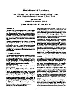
One experiment was a three-way join of Orders relations. The join was on the orderkey and produced 15 million results. The results are in Figure 4.2 1

The TPC-H data set scale factor 100 GB was tested on the hardware but run times of many hours to days made it impractical for the tests.

31

4.1. PostgreSQL Results Relation Customer Supplier Part Orders PartSupp LineItem

Tuple 194 184 173 147 182 162

Size B B B B B B

#Tuples 1.5 million 100,000 2 million 15 million 8 million 60 million

Relation Size 284 MB 18 MB 323 MB 2097 MB 1392 MB 9270 MB

Figure 4.1: TPC-H 10 GB Relation Sizes (time) and Figure 4.3 (IOs). In these figures, Hybrid Hash Join referred to as HHJ was compared with Hash Teams referred to as N-way (direct). 300

700 680

250

660 640 Time (sec)

Time (sec)

200

150

100

620 600 580 560 540

50

520

HHJ N-way (direct) 0

500 0

500

1000 1500 2000 Memory Size (MB)

2500

3000

0

Figure 4: Three Way Orders Join (Time) Figure 4.2: Time for Three Way Orders Join

500

1000 Me

Figure 6: Part-Par 25000

20000

I/Os (MB)

I/Os (MB)

The results 20000clearly show a benefit for a multi-way join with about a 60% HHJ reduction in I/O bytes for the join and approximately 12-15% improvement N-way (direct) 18000 in overall time. The multi-way join performs fewer I/Os by saving one partitioning16000 step. It also saves by not materializing intermediate tuples in 14000 memory and by reducing the number of probes performed. The multi-way join continues 12000to be faster even for larger memory sizes and a completely in-memory 10000 join. Another direct partitioning join hashes Part, PartSupp and LineItem 8000 on partkey and joins PartSupp and LineItem on both partkey and suppkey. The results 6000 are in Figure 4.4 (time) and Figure 4.5 (IOs). In this test

15000

10000

5000

4000

32

2000

0 0

0 0

500

1000 1500 2000 Memory Size (MB)

2500

3000

Figure 5: Three Way Orders Join (I/O bytes)

500

1000 M

Figure 7: Part-PartS

The result was only a 2% i

580 100

560 540

50

520

HHJ N-way (direct) 0

500 0

500

1000 1500 2000 Memory Size (MB)

2500

3000

0

4.1. PostgreSQL Results Figure 4: Three Way Orders Join (Time)

500

1000 Memo

Figure 6: Part-PartS 25000

20000 HHJ N-way (direct)

18000

20000 16000 I/Os (MB)

I/Os (MB)

14000 12000 10000

15000

10000

8000 6000 5000 4000 2000 0 0

0 0

500

1000 1500 2000 Memory Size (MB)

2500

3000

500

1000 Mem

Figure 7: Part-PartSup

Figure 5: Three Way Orders Join (I/O bytes) Figure 4.3: I/O Bytes for Three Way Orders Join

The result was only a 2% imp The clear impact of probi HHJ was Another compareddirect against Hash Teams using lazy materialization (N-way partitioning join hashes Part, PartSupp vate the benefit of adaptive pr (direct,lazy)) as well as Hash Teams using eager materialization (N-way and LineItem on partkey and joins PartSupp and LineItem which may improve results. C (direct,eager)). on both partkey and suppkey. The results are in Figure 6 a secondary factor to I/Os fo To test theand potential (time) Figure benefit 7 (IOs).of eager materialization, we modified the practice the costs can be quit Unlike to theallow one-to-one join, this join exhibited different implementation for materialization of intermediate tuples unconbased on theThus, implementations. The original strainedperformance by memory limitations. the materialization implementation 6.2 Indirect Partitioni implementation (not shown)exceed had the join being is unrealistically good as it could themulti-way space allocated for the joinIndirect partitioning was te slowerwithout over all paying memoryany sizes by 5-20% though it had considerably extra I/O oreven memory costs. The result Orders, and LineItem. We te performed significantly less I/O. The difference turned out 2 was only a 2% improvement in time . with no hybrid component, to be significantly more hash and join qualifier (clause) evalUnlike the one-to-one join, this join exhibited different performance brid component, a bit mapp uations for the multi-way operator. Several optimizations and HHJ. The bit mapper wi based on the implementations. The original implementation (not shown) were made to reduce the number of qualifier evaluations and its entire memory allocation d had theprobes multi-way join being slower over all memory sizes by 5-20% even to below that of HHJ. The multi-way join does not mapper. The hybrid bit map though have it had performed significantly I/O. Thesizes. difference turned out superior performance over less all memory The maof tuples in the Orders relatio to be significantly more in hash and (clause) jor improvement I/Os atjoin 500 qualifier MB is due to the evaluations multi-way for the the same amount of space use operator sharing memory between the inputs smaller multi-way operator. Several optimizations were madeastothe reduce the number results are in Figure 8 (time) inputevaluations Part fits inand its 500 MBto allocation and of can provide of qualifier probes below that HHJ. Thean multi-way For this join, the multi-way extra to buffer PartSupp over tuples. join does not 187 haveMB superior performance all memory sizes. The major that To test the potential benefit eager we sharing did not always translate t improvement in I/Os at 500 MB is dueof to the materialization, multi-way operator difference was large. The hyb to allowinput for materialization of 500 MB memorymodified betweenthe theimplementation inputs as the smaller Part fits in its the join memory increases. HH intermediate tuples unconstrained by memory limitations. allocation and can provide an extra 187 MB to buffer PartSupp tuples. memory jump from 2000 MB t Thus, the materialization implementation is unrealistically 2

good as it could exceed thetospace allocated formore theclearly. join conThe y-axis origin is at 500 seconds show the difference siderably without paying any extra I/O or memory costs.

2

The y-axis origin is at 500 s more clearly.

33

4.1. PostgreSQL Results

700 680 660

Time (sec)

640 620 600 580 560 540 HHJ N-way (direct,lazy) N-way (direct,eager)

520 500 0

500

1000 1500 2000 Memory Size (MB)

2500

3000

Figure 4.4: Time for Part-PartSupp-Lineitem

25000 HHJ N-way (direct)

I/Os (MB)

20000

15000

10000

5000

0 0

500

1000 1500 2000 Memory Size (MB)

2500

3000

Figure 4.5: I/O Bytes for Part-PartSupp-Lineitem

34

4.1. PostgreSQL Results The clear impact of probing cost on the results motivate the benefit of adaptive probe orders (not implemented) which may improve results. CPU costs are often considered a secondary factor to I/Os for join algorithms, although in practice the costs can be quite significant.

4.1.2

Indirect Partitioning with Generalized Hash Teams

Indirect partitioning was tested with a join of the Customer, Orders, and LineItem relations. We tested the original bit mapper with no hybrid component, an exact mapper with a hybrid component, a bit mapper with a hybrid component, and HHJ. The bit mapper with no hybrid component used its entire memory allocation during partitioning for the bit mapper. The hybrid bit mapper used 12 bytes * number of tuples in the Orders relation as its bit map size which is the same amount of space used by the exact mapper. The results are in Figure 4.6 (time) and Figure 4.7 (IOs). 1100 1000

Time (sec)

900 800 700 600 HHJ N-way (exact,hybrid) N-way (bitmap,no hybrid) N-way (bitmap,hybrid)

500 400 0

500

1000 1500 2000 Memory Size (MB)

2500

3000

Figure 4.6: Time for Customer-Orders-LineItem For this join, the multi-way algorithms had fewer I/Os but that did not always translate to a time advantage unless the difference was large. The hybrid stage is a major benefit as the join memory increases. HHJ had worse performance on a memory jump from 2000 MB to 2500 MB despite performing 20GB fewer I/Os! The difference was the optimizer changed the query plan to join Orders with LineItem then the result with Customer at 2500 MB where previously Customer and Orders were joined first. This new 35

4.1. PostgreSQL Results 35000 HHJ N-way (exact,hybrid) N-way (bitmap,no hybrid) N-way (bitmap,hybrid)

30000

I/Os (MB)

25000 20000 15000 10000 5000 0 0

500

1000 1500 2000 Memory Size (MB)

2500

3000

Figure 4.7: I/O bytes for Customer-Orders-LineItem ordering produced double the number of probes and join clause evaluations and ended up being slower overall. The major limitation was the mapper size. The mappers did not produce results for the smaller memory sizes of 32 MB and 64 MB as the mapper could not be memory-resident. For 128 MB, the bit mapper performed significantly more I/Os and had larger time than the exact mapper due to the number of false drops. The number of false drops was greatly reduced as the memory increased. The bit mapper without a hybrid component continued to read/write all relations and was never faster than HHJ.

4.1.3

Multi-Dimensional Partitioning with SHARP

One of the star join tests combined Part, Orders, and LineItem. The performance of the SHARP algorithm versus hybrid hash join is in Figures 4.8 and 4.9. SHARP performed 50-100% fewer I/Os in bytes and was about 5-30% faster. Only at very small memory sizes did the performance become slower than HHJ, and it was faster in the full memory case.

36

4.1. PostgreSQL Results

1400 1200

500 2000 2500 HHJ SizeN-way (MB) (exact,hybrid) N-way (bitmap,no hybrid) N-way (bitmap,hybrid)

Time (sec)

HHJ N-way (exact,hybrid) N-way (bitmap,no hybrid) N-way (bitmap,hybrid)

1200 800

Time (sec)

1400 1000

800 400

1000 600

2500

3000

0

1000 1500 2000 Memory Size (MB)

2500

3000

HHJ N-way (multi)

0 Figure 10: Part-Orders-LineItem (time) 0 500 1000for Part-Orders-LineItem 1500 2000 2500 Figure 4.8: Time

3000

3000

Memory Size (MB)

90000

Figure 80000

I/Os (MB)

I/Os (MB)

HHJ N-way (exact,hybrid) N-way (bitmap,no hybrid) N-way (bitmap,hybrid)

2500

3000

70000 90000 60000 80000 50000 70000 40000 60000 30000 50000 20000 40000 10000 30000 0 20000 0

HHJ

N-way (multi) 10: Part-Orders-LineItem (time)

HHJ N-way (multi)

500

10000

rs-LineItem (I/O bytes)

1500 2000 ry Size (MB)

500

200

HHJ(Time) ders-LineItem N-way (exact,hybrid) N-way (bitmap,no hybrid) N-way (bitmap,hybrid)

1500 2000 y Size (MB)

HHJ N-way (multi)

400 0

ders-LineItem (Time)

1500 2000 y Size (MB)

600 200

2500

3000

e was the optimizer rs-LineItem (I/O changed bytes) ith LineItem then the result ere previously Customer and ew ordering producedchanged double ce was the optimizer clause evaluations and with LineItem then theended result

ere previously Customer and he The double mapewmapper orderingsize. produced or the smaller memory sizes clause evaluations and ended apper could not be memorythemapper mapperperformed size. Thesignifimaptime than the mapper or the smaller exact memory sizes s.apper The could number false drops notofbe memory-

1000 1500 2000 Memory Size (MB)

2500

3000

0 Figure 11: Part-Orders-LineItem (I/O bytes) 0

500

1000 1500 2000 Memory Size (MB)

2500

3000

6.4 Figure Results 11: Discussion Part-Orders-LineItem (I/O bytes)

Figure joins 4.9: I/O for to Part-Orders-LineItem Multi-way can Bytes be added the optimizer using postoptimization. Post-optimization has a low barrier to entry and manyDiscussion of the opportunities for exploiting multi6.4 catches Results way joins. The cost functions allow theoptimizer optimizerusing to choose Multi-way joins can be added to the postbetween the binary and multi-way operators. optimization. Post-optimization has a low barrier to entry Implementing efficient, robust, and for scaleable multi-way and catches many of the opportunities exploiting multijoins is a non-trivial challenge. Multi-way joins being adapway joins. The cost functions allow the optimizer to choose tive is great, but it is ideal if they also have improved or between the binary and multi-way operators. comparable performance to binary plans when the optimizer Implementing efficient, robust, and scaleable multi-way isjoins “correct” in its optimization. The experimental is a non-trivial challenge. Multi-way joins beingresults adapclearly show that multi-way performance depends on the tive is great, but it is ideal if they also have improved or join type. Direct partitioning joins arewhen efficient and are comparable performance to binary plans the optimizer

37

4.2. Standalone C++ Results

4.2

Standalone C++ Results

The standalone implementation of the join algorithms allows for the algorithms to be tested in isolation from their environment. This allows for the algorithms to be tested without the overhead of the caching and memory management of PostgreSQL. Each aspect of the test can be easily controlled. All experiments were performed on a PC running Windows 8 with a quad core Intel Core i7 2600K processor at 4.4GHz with 24GB RAM and a 512 GB Crucial M4 solid state drive.

4.2.1

Database Schema

The database used to compare the algorithms was a 10GB TPC-H [tpc] database. Figure 4.1 describes the size of each relation.

4.2.2

Direct Partitioning with Hash Teams

Hash Teams was compared to DHJ using the query in Listing 4.1. Both left deep and right deep DHJ query plans were evaluated. The query was repeated ten times for each memory size. The amount of memory for each operator in the join plan was calculated using the following formula. memory = memorySize ∗ (n − 1) where n is the number of inputs to the operator. Since DHJ is a binary operator, both DHJ operators in the join plan were given memorySize bytes of memory. Hash Teams is a n-ary operator. Since Hash Teams had three inputs the solitary hash team received 2 × memorySize bytes of memory. Listing 4.1: Query for a Three Way Join on the Orders Relation s e l e c t ∗ from Orders o1 , Orders o2 , Orders o3 where o1 . o r d e r k e y = o2 . o r d e r k e y and o2 . o r d e r k e y = o3 . o r d e r k e y ; Figure 4.11 shows that Hash Teams performed 50% to 100% fewer I/Os than the left deep DHJ query. The right deep DHJ query is able to perform zero I/Os for the same memory sizes but the I/Os increase at a much faster rate than Hash Teams. The right deep plan uses fewer I/Os than the left deep plan because it always chooses a single Order relation to partition for both DHJ operators while the second operator in the left deep plan partitions the result of the first DHJ operator. Figure 4.10 shows that Hash Teams performed 20% faster than the right deep DHJ plan at all memory sizes and up to 42% faster than the left 38

4.2. Standalone C++ Results

120 DHJ Left Deep DHJ Right Deep

100

Time (sec)

Hash Teams 80

60

40

20

0

391

781 1172 1563 1953 2344 2734 3125 3516 3906 4297 4688

Memory Size (MB)

Figure 4.10: Time for 3-Way TPC-H Order Join

20000 DHJ Left Deep

18000

DHJ Right Deep

16000

Hash Teams

I/Os (MB)

14000

12000 10000 8000 6000 4000

2000 0 391

781 1172 1563 1953 2344 2734 3125 3516 3906 4297 4688

Memory Size (MB)

Figure 4.11: I/O Bytes for 3-Way TPC-H Order Join

39

4.2. Standalone C++ Results deep DHJ plan. This is mostly due to DHJ requiring multiple partitioning steps and intermediate tuple materialization. Since Hash Teams only has one partitioning step and only materializes tuples when producing the final output it is able to gain a significant advantage over the widely used dynamic hash join.

4.2.3

Indirect Partitioning with Generalized Hash Teams

Generalized Hash Teams (GHT) were compared to DHJ using the query in listing 2.4. Both left deep and right deep DHJ query plans were evaluated. The query was repeated five times for each memory size. First, GHT was evaluated using a large amount of memory for the map in order to ensure that there were no false drops. This is to show the behaviour of GHT in its best possible conditions as the memory for the map is not counted against the memory for the join. Second, GHT was evaluated with the map memory counted against the join memory to show its behaviour in normal conditions. The memory sizes were calculated the same way as in Section 4.2.2.

180 DHJ Left Deep

160

DHJ Right Deep

Time (sec)

140

GHT

120 100 80

60 40 20

0 391 781 1172 1563 1953 2344 2734 3125 3516 3906 4297 4688

Memory Size (MB)

Figure 4.12: Time for 3-Way TPC-H Customer, Orders, Lineitem Join Figure 4.13 shows that Generalized Hash Teams performed 70% to 100% fewer I/Os than the left deep DHJ query. The GHT query is able to perform zero I/Os for the lower memory sizes. The right deep DHJ query performs 40

4.2. Standalone C++ Results

30000 DHJ Left Deep DHJ Right Deep

25000

GHT

I/Os (MB)

20000 15000 10000 5000 0 391 781 1172 1563 1953 2344 2734 3125 3516 3906 4297 4688

Memory Size (MB)

Figure 4.13: I/O Bytes for 3-Way TPC-H Customer, Orders, Lineitem Join fewer I/Os than the left deep plan since it avoids partitioning the intermediate result tuples but it still performs more I/Os than GHT because it is less efficient in its use of memory. Figure 4.12 shows that GHT is approximately 8% slower than the right deep DHJ plan when performing zero I/Os and 25% slower than the left deep DHJ plan. GHT is slower because of the extra hashing and probing of the map GHT needs to match tuples when joining relations. It is not until low memory sizes that GHT becomes faster than both the left and right deep DHJ plans. Figure 4.15 shows the I/Os used for GHT when the memory used by the map is removed from the memory available to the join. GHT behaves reasonably until there is not enough memory to keep the number of false drops low. Once GHT has only a very small amount of memory the mapping places each Lineitem tuple in a large number of partitions causing the amount of file I/O to increase significantly. Figure 4.14 shows that once the I/Os increase for GHT it becomes the slowest join. Figure 4.17 shows the effect of the number of bits per tuple that is used for the map. When there is a small amount of memory available for the map (approximately 1 bit for every 10 tuples) the number of false drops becomes very large. Figure 4.16 shows the effect of the bitmap size on the runtime 41

4.2. Standalone C++ Results

500 DHJ Left Deep

450

DHJ Right Deep

400

GHT

Time (sec)

350 300 250 200 150

100 50 0 39

78

117

156

195

234

273

313

352

Memory Size (MB)

Figure 4.14: Time for 3-Way TPC-H Customer, Orders, Lineitem Join with Small Memory Sizes

70000

DHJ Left Deep DHJ Right Deep

60000

GHT

I/Os (MB)

50000 40000 30000 20000 10000

0 39

78

117

156

195

234

273

313

352

Memory Size (MB)

Figure 4.15: I/O Bytes for 3-Way TPC-H Customer, Orders, Lineitem Join with Small Memory Sizes 42

4.2. Standalone C++ Results

400 350

Time (sec)

300 250 200

150 100 50 0 0.1

0.25

0.5

1

1.5

Bitmap Size Multiplier

2

4

Figure 4.16: Time for Bitmap Size with 3-Way TPC-H Customer, Orders, Lineitem Join

400000000 350000000

False Drops

300000000 250000000 200000000 150000000 100000000

50000000 0 0.1

0.25

0.5

1

1.5

2

4

Bitmap Size Multiplier

Figure 4.17: False Drops for Bitmap Size with 3-Way TPC-H Customer, Orders, Lineitem Join 43

4.2. Standalone C++ Results of the algorithm.

4.2.4

Multi-Dimensional Partitioning with SHARP

SHARP was compared against DHJ using the query in listing 4.2. In this star join, Lineitem is the fact table and Orders and Part are the dimension tables. The query was repeated ten times for each memory size. As shown in Figure 4.19 SHARP is able to make much more efficient use of the join memory to perform fewer I/Os in low memory conditions. This is because SHARP partitions each relation independently. Since SHARP performs fewer I/Os and does not need multiple partitioning steps, it is faster than DHJ at all memory sizes as shown in Figure 4.18. Listing 4.2: Three Way Star Join Query on the Orders, Part and Lineitem Relations s e l e c t ∗ from Orders o , Part p , L i n e i t e m l where o . o r d e r k e y = l . o r d e r k e y and p . p a r t k e y = l . p a r t k e y ;

350 SHARP

300

DHJ

Time (sec)

250 200

150 100 50 0

391

781

1172

1563

1953

2344

Memory Size (MB)

Figure 4.18: Time for 3-Way Star Join on Orders, Part, and Lineitem

44

4.2. Standalone C++ Results

45000 SHARP

40000

DHJ

35000

I/Os (MB)

30000 25000 20000 15000

10000 5000 0 391

781

1172

1563

Memory Size (MB)

1953

2344

Figure 4.19: I/O Bytes for 3-Way Star Join on Orders, Part, and Lineitem

45

Chapter 5

Discussion and Conclusion The storage, retrieval and analysis of large amounts of data is very common. Since large data sets can take a very large amount of time to process, there has been a large amount of research to find faster ways to process this data. Faster join algorithms reduce the amount of time it takes to analyse data sets which make it possible to process even larger data sets in a reasonable amount of time. The goals presented in Chapter 1 of this thesis were to determine if Hash Teams, Generalized Hash Teams, or SHARP improve the efficiency of the standard hash joins in relational database systems and if it makes sense to implement them. The experiments performed allowed each of the algorithms to be tested directly against the standard hash joins in terms of both run time efficiency and algorithmic complexity. Hash Teams is a simple multi-way hash join that has a performance benefit over dynamic hash join (DHJ). The experiments show that it outperforms DHJ since it is able to avoid the intermediate partitioning step of DHJ and can use memory more efficiently than DHJ. However, there are only a very limited number of queries that Hash Teams can be used for. In many cases a standard merge join would be more efficient than Hash Teams for these queries where the data is already sorted. Hash teams is also more complex to implement and maintain than DHJ. Because of the limited use and complexity of Hash Teams it is not recommended to be implemented in a database management system. This is also supported by Microsoft dropping Hash Teams support in SQL Server 2003. Generalized Hash Teams (GHT) can be used for a significantly larger number of queries than Hash Teams. However, GHT is also much more complex as it requires a mapper for indirect queries. The experiments show that it also has a limited performance benefit in a small number of cases but actually performs worse than DHJ in others. Due to its high complexity and potential for poor performance, Generalized Hash Teams is not recommended to be implemented in a relational database management system. SHARP shows a significant benefit over DHJ. The experimental results show that it performs fewer I/Os and is faster than DHJ. It is more efficient 46

Chapter 5. Discussion and Conclusion in its use of the memory available for the join. A disadvantage is that it can only be used for star queries which means it cannot be used for most normal queries. However, star queries are very commonly used in data warehousing. Data warehousing is often used to store historical data such as sales transactions. For large companies such as Wal-Mart this means they need to store and analyze multi-terabyte data sets. Because the database sizes for data warehousing are usually very large, joins are also very slow. Any increase in join efficiency can have a large impact. SHARP should be implemented in database management systems that are used for data warehousing. This thesis has shown that even though multi-way hash joins can perform fewer I/Os than traditional binary hash joins, they are quite limited in their use in practice. Only SHARP can be recommended since it shows a significant advantage in its relevant queries. Hash teams and Generalized Hash Teams are too limited and complicated to be very useful in a relational database management system. Future work includes experiments on the algorithms with a larger number of relations in a single query. It also includes experiments with different queries on other data sets. Future work for Hash Teams and Generalized Hash teams includes implementing and experimenting with the GROUP BY operator for use with the joins to see if it makes the algorithms more useful. It is also possible to perform a study on how parallization of the algorithms would affect their relative performance.

47

Bibliography [BD06] Pedro Bizarro and David J. DeWitt. Adaptive and Robust Query Processing with SHARP. Technical Report 1562, University of Wisconsin, 2006. → pages 2, 22, 27 [BLP11] Spyros Blanas, Yinan Li, and Jignesh M. Patel. Design and Evaluation of Main Memory Hash Join Algorithms for Multi-Core CPUs. In Proceedings of the 2011 ACM SIGMOD International Conference on Management of data, SIGMOD ’11, pages 37–48, New York, NY, USA, 2011. ACM. → pages 15 [CGN10] Shimin Chen, Phillip B. Gibbons, and Suman Nath. PR-Join: A Non-Blocking Join Achieving Higher Early Result Rate with Statistical Guarantees. In Proceedings of the 2010 ACM SIGMOD International Conference on Management of data, SIGMOD ’10, pages 147–158, New York, NY, USA, 2010. ACM. → pages 14 [CM03] Gene Cooperman and Xiaoqin Ma. DPG: A Cache-Efficient Accelerator for Sorting and for Join Operators. CoRR, cs.DB/0308004, 2003. → pages 15 [CN] S. Chaudhuri and V. Narasayya. TPC-D Data Generation with Skew. Technical report, Microsoft Research, Available at: ftp.research.microsoft.com/users/viveknar/tpcdskew. → pages 31 [Cod70] E. F. Codd. A Relational Model of Data for Large Shared Data Banks. Commun. ACM, 13(6):377–387, 1970. → pages 6 [Dat94] C. Date. The SQL Standard. Addison Wesley, Reading, US, third edition, 1994. → pages 7 [DKO+ 84] D. DeWitt, R. Katz, F. Olken, L. Shapiro, M. Stonebraker, and D. Wood. Implementation Techniques for Main Memory Database Systems. In ACM SIGMOD, pages 1–8, 1984. → pages 11

48

Bibliography [DN95] D. DeWitt and J. Naughton. Dynamic Memory Hybrid Hash Join. Technical report, University of Wisconsin, 1995. → pages 1, 11 [DSTW02] J.-P. Dittrich, B. Seeger, D. Taylor, and P. Widmayer. Progressive Merge Join: A Generic and Non-Blocking Sort-based Join Algorithm. In VLDB 2002, pages 299–310, 2002. → pages 14 [DSTW03] Jens-Peter Dittrich, Bernhard Seeger, David Scot Taylor, and Peter Widmayer. On Producing Join Results Early. In Proceedings of the twenty-second ACM SIGMOD-SIGACT-SIGART symposium on Principles of database systems, PODS ’03, pages 134–142, New York, NY, USA, 2003. ACM. → pages 14 [GBC98] Goetz Graefe, Ross Bunker, and Shaun Cooper. Hash Joins and Hash Teams in Microsoft SQL Server. In VLDB, pages 86–97, 1998. → pages 2, 16, 18 [Gra93] G. Graefe. Query Evaluation Techniques for Large Databases. ACM Computing Surveys, 25(2):73–170, 1993. → pages 8 [Gra99] Goetz Graefe. The Value of Merge-Join and Hash-Join in SQL Server. In Proceedings of the 25th International Conference on Very Large Data Bases, VLDB ’99, pages 250–253, San Francisco, CA, USA, 1999. Morgan Kaufmann Publishers Inc. → pages 7 [HCL09] Michael Henderson, Bryce Cutt, and Ramon Lawrence. Exploiting Join Cardinality for Faster Hash Joins. In Proceedings of the 2009 ACM symposium on Applied Computing, SAC ’09, pages 1549–1554, New York, NY, USA, 2009. ACM. → pages 14 [Hen] Michael Henderson. C++ Source Code for Multi-Way Join Algorithms. https://bitbucket.org/mikecubed/hashjoins. → pages 29 [HH99] Peter J. Haas and Joseph M. Hellerstein. Ripple Joins for Online Aggregation. In Proceedings of the 1999 ACM SIGMOD international conference on Management of data, SIGMOD ’99, pages 287–298, New York, NY, USA, 1999. ACM. → pages 14 [HWM98] Sven Helmer, Till Westmann, and Guido Moerkotte. Diag-Join: An Opportunistic Join Algorithm for 1:N Relationships. In Proceedings of the 24rd International Conference on Very Large 49

Bibliography Data Bases, VLDB ’98, pages 98–109, San Francisco, CA, USA, 1998. Morgan Kaufmann Publishers Inc. → pages 14 [KKL+ 09] Changkyu Kim, Tim Kaldewey, Victor W. Lee, Eric Sedlar, Anthony D. Nguyen, Nadathur Satish, Jatin Chhugani, Andrea Di Blas, and Pradeep Dubey. Sort vs. Hash Revisited: Fast Join Implementation on Modern Multi-Core CPUs. Proc. VLDB Endow., 2(2):1378–1389, August 2009. → pages 15 [KKW99] Alfons Kemper, Donald Kossmann, and Christian Wiesner. Generalised Hash Teams for Join and Group-by. In VLDB, pages 30–41, 1999. → pages 2, 18, 20 [KNT89] Masaru Kitsuregawa, Masaya Nakayama, and Mikio Takagi. The Effect of Bucket Size Tuning in the Dynamic Hybrid GRACE Hash Join Method. In VLDB, pages 257–266, 1989. → pages 12 [KTMo83] M. Kitsuregawa, H. Tanaka, and T. Moto-oka. Application of Hash to Database Machine and Its Architecture. New Generation Computing, 1(1), 1983. → pages 10 [Law05] Ramon Lawrence. Early Hash Join: A Configurable Algorithm for the Efficient and Early Production of Join Results. In VLDB 2005, pages 841–852, 2005. → pages 14 [Law08] Ramon Lawrence. Using Slice Join for Efficient Evaluation of Multi-Way Joins. Data and Knowledge Engineering, 67(1):118– 139, October 2008. → pages 27 [LEHN02] Gang Luo, Curt J. Ellmann, Peter J. Haas, and Jeffrey F. Naughton. A Scalable Hash Ripple Join Algorithm. In Proceedings of the 2002 ACM SIGMOD international conference on Management of data, SIGMOD ’02, pages 252–262, New York, NY, USA, 2002. ACM. → pages 14 [LKM08] Justin J. Levandoski, Mohamed E. Khalefa, and Mohamed F. Mokbel. PermJoin: An Efficient Algorithm for Producing Early Results in Multi-join Query Plans. In Proceedings of the 2008 IEEE 24th International Conference on Data Engineering, ICDE ’08, pages 1433–1435, Washington, DC, USA, 2008. IEEE Computer Society. → pages 14

50

Bibliography [MLA04] M. Mokbel, M. Lu, and W. Aref. Hash-Merge Join: A NonBlocking Join Algorithm for Producing Fast and Early Join Results. In ICDE, pages 251–263, March 2004. → pages 14 [NKT88] Masaya Nakayama, Masaru Kitsuregawa, and Mikio Takagi. Hash-Partitioned Join Method Using Dynamic Destaging Strategy. In VLDB, pages 468–478, 1988. → pages 1, 11 [OG95] Patrick E. O’Neil and Goetz Graefe. Multi-Table Joins Through Bitmapped Join Indices. SIGMOD Record, 24(3):8–11, 1995. → pages 15 [Pos] PostgreSQL. Open Source Relational Database Management System. http://www.postgresql.org/. → pages 27 [tpc] TPC-H Benchmark. Technical report, Transaction Processing Performance Council. http://www.tpc.org/tpch/. → pages 19, 31, 38 [UF00] T. Urhan and M. Franklin. XJoin: A Reactively Scheduled Pipelined Join Operator. IEEE Data Engineering Bulletin, 23(2):7–18, 2000. → pages 14 [ZG90] H. Zeller and J. Gray. An Adaptive Hash Join Algorithm for Multiuser Environments. In VLDB 1990, pages 186–197, 1990. → pages 9, 12

51