Monetary Policy Rules at the Bank of England

Kalin Nikolov# Bank of England June 2002

#

Monetary Assessment and Strategy Division, Bank of England

This paper was prepared for the workshop on ‘The Role of Policy Rules in the Conduct of Monetary Policy’ held at the European Central Bank in Frankfurt, March 11-12, 2002. It draws on the work of many colleagues, past and present, at the Bank of England. I am particularly grateful to Peter Andrews, Kosuke Aoki, Mark Astley, David England and Phil Evans for comments and assistance with previous versions of this paper. The views expressed are those of the author and do not reflect the views of either the Bank of England or the Monetary Policy Committee.

1

1. Introduction

This contribution outlines the way the Bank of England uses monetary policy rules. It explains why, in common with other central banks, the Bank does not use mechanical instrument rules to set policy but instead uses a ‘targeting rule’ – an inflation target – both to implement and communicate policy. We argue that objectives defined in terms of inflation outcomes offer the right combination of a clear commitment to the goal of low inflation with the necessary flexibility to respond to shocks in an appropriate manner. We explain how the Bank nevertheless uses policy rules as one input in its regular assessment of the stance of policy and how its research into the behaviour of policy rules under different assumptions about the structure of the economy can give insights into the conduct of policy.

The paper is organised as follows. Section 2 outlines some of the advantages and disadvantages of commitment to a monetary policy rule. Section 3.1 explains how the Bank of England sets policy, paying particular attention to the reasons why mechanical rules would be inappropriate in the context of the UK’s inflation targeting framework. Section 3.2 outlines some of the policy and research applications of the monetary policy rules literature with the Bank. Section 4 concludes.

2. Advantages and disadvantages of instrument rules

A debate on ‘rules’ versus discretion arose within the context of weak monetary policy credibility in the 1970s. The problem was articulated along the following lines: since monetary authorities have other objectives apart from low inflation (for example, high employment), they may be tempted to generate a boom that reduces unemployment in the short run although it eventually leads to higher inflation. Rational agents accordingly set their inflation expectations at a level such that the costs to the central bank from further inflation are higher than the benefits from reducing unemployment. In the resulting equilibrium inflation is inefficiently high due to the lack of credibility on the part of monetary policy.

Since the lack of credibility stems from the discretion afforded to the central bank, the literature has recommended that the monetary authority commit itself to a rule, which 2

is consistent with low inflation. There are a number of such candidate ‘instrument’ or ‘intermediate’ rules: the Taylor rule, the McCallum rule, and Friedman’s constant money growth rate rule to name but a few. Adherence to such a rule, the argument goes, will strengthen the central bank’s credibility and anchor inflation expectations at low levels1.

In the 1990s, following the sustained world-wide disinflation, academic and policymaker interest shifted to the design of monetary policy rules which generate equilibria with desirable features, such as low inflation and output volatility. Below we examine the advantages and disadvantages of instrument rules against two main criteria: transparency (are the rules easy to communicate to the public?) and optimality (do the rules deliver good economic outcomes?). •

Simple rules

Simple feedback instrument rules such as the Taylor (1993) rule involve a reaction to variables such as inflation and the output gap, which are considered intuitively relevant to the conduct of monetary policy. Their great virtue is simplicity, which makes them easy to understand. Simple rules could be used in central bank communication although the public will not be able to verify the exact rule that is being followed if the monetary authority does not publish all the information required, such as its estimate(s) of the output gap. And Taylor (1999) has argued that the Taylor rule performs well in a wide range of models, which makes it robust to model uncertainty.

Despite all the above advantages, simple rules have a number of weaknesses. Although their performance is rarely disastrous (as long as the coefficient on inflation in the nominal interest rate rule is above unity2), they can involve large welfare losses relative to fully optimal rules. And some studies (for example, Batini, Harrison and Millard (2001)) have argued that Taylor type rules are not robust to open economy features. 1

Of course, such an argument does not explain how the monetary authority will be able to commit itself to a monetary rule. 2 If the coefficient on inflation is below unity, then in backward-looking models, inflation will be explosive, while in forward-looking models, inflation could be driven by self-fulfilling inflation

3

•

Fully optimal rules

Fully optimal rules are generally derived from the first order conditions of the central bank’s welfare maximisation subject to its model of the economy. They represent the minimum welfare loss given the structure of the economy and the variability of the shocks hitting it. Woodford (2000) shows that the fully optimal rule involves a commitment by the central bank to a contingent plan for the future path of interest rates, which allows it to stabilise private sector expectations and consequently control inflation at a lower cost in terms of output volatility In practice this will introduce interest rate smoothing into the policy rule followed by the monetary authority.

But optimal rules are derived subject to a given model of the economy. This makes them very sensitive to the particular assumptions underlying the model. For example, models with forward-looking agents tend to imply rules with a lot of history dependence since the monetary authority wants to influence private sector expectations in line with its objectives. In contrast, ‘mechanical’ (backward-looking) models do not have this implication and instead tend to favour forward-looking rules. Hence, optimal monetary policy rules are not robust to model uncertainty. Furthermore, as Svensson (2001) shows, optimal rules will in general be very complex, making it difficult for the private sector to monitor whether the rule really is being followed.

So, both simple and optimal instrument rules have their advantages and disadvantages. Simple rules are easy to explain and monitor, providing the public with the reassurance that the central bank is committed to low inflation, and is not about to spring an inflation surprise on the economy. But they are rarely optimal. Optimal rules (by definition) deliver the best performance but they are model sensitive and may be difficult to communicate.

And crucially, both optimal and simple instrument rules imply a mechanical link between the policy rate and information available to the central bank, which is perhaps the reason why no central bank has so far committed itself to following one of them. In contrast, a number of central banks have adopted ‘targeting rules’ similar expectations. When the inflation coefficient is above unity, inflation is stable and driven only by fundamentals in both forward and backward-looking models.

4

to the UK’s inflation targeting regime. In the next section, we offer our view of why a ‘targeting rule’ is superior to instrument rules in maintaining public confidence while giving monetary authorities the flexibility to stabilise the economy in an optimal way.

3. How the Bank of England uses monetary policy rules?

3.1. The Bank of England’s ‘inflation targeting rule’

Although the Bank of England does not set policy using a particular mechanical policy rule, the UK policy framework is firmly grounded on a commitment to low inflation. Since the Bank was given operational independence in June 1997, it has had a statutory duty, set out in the Bank of England Act of 1998, to keep inflation3 as close as possible to a target set by the Chancellor. The target has remained at 2.5% since the Bank was granted independence, although it is reviewed annually at each Budget speech. The target applies at all times.

Members of the MPC are individually accountable to Parliament for meeting the inflation target. Therefore, although the Bank does not follow an explicit rule for the policy rate, the UK’s institutional framework has ensured that the post-1997 regime enjoys a great deal of credibility. Indeed, most measures of inflation expectations have remained very close to target despite large swings in exchange rates and oil and commodity prices.

Due to the significant lags in the transmission of monetary policy, the MPC bases its monetary policy decisions upon its forecasts of inflationary pressures in the economy. Each quarter the Committee formulates a projection for inflation and GDP over a twoyear period using the Bank’s Macroeconomic Model and whatever other models and information is available to inform its judgment. The Committee uses a constant interest rate path as a working assumption in generating the projections.4 The most likely path or ‘central projection’ is the modal scenario in the Bank’s Inflation Report 3

The 12-month rate of increase of RPIX, the index of retail prices excluding mortgage interest payments. 4 Although the Committee also considers projections based on market interest rate expectations.

5

fan chart. Historical forecast errors and the MPC’s judgment on the degree of uncertainty in the economy going forward determines the variance of the fan chart. Finally, the MPC’s views on the balance of risks to economic activity and inflationary pressure are used to set the skews of the fan chart.

The resulting distribution of expected inflation and output growth over the two-year period following each forecast is a key ingredient in the MPC’s policy decisions. But although the inflation projection is key in the execution and communication of monetary policy in the UK, there is no simple mechanical link between the central projection and policy decisions. The MPC takes a number of additional considerations into account when setting policy.

The prospects for real activity matter. Although the 1998 Bank of England Act places price stability (defined by the Chancellor’s inflation target) as the overriding objective of monetary policy , the Bank of England is also required to support the Government’s other economic goals. What this has implied in practice is that the Bank has an obligation to consider the resulting volatility of real activity when setting interest rates. So, for example, if a shock to oil prices were to occur, increasing inflation and depressing real activity, the Bank might choose to bring inflation back to target gradually to avoid extreme output costs in the short term.

The uncertainty around the central projection is important in reaching policy decisions. As the November 2000 Inflation Report (page 67) states, this will ‘’…tend to encourage more cautious decisions.’

The MPC also cares about the balance of risks around the central projection. On this point, King (2001) argues that: ‘…in some circumstances it may make sense to focus very much on the mean outlook, and there is no doubt that over a long period any deviation from that must cancel out if the target is to be met on average.’

6

In practice, the February 2002 MPC Minutes stress that ‘…the economic factors and analysis behind the fan chart’ are crucial in determining whether policy responds or not to the balance of risks around the central projection.

‘…the fan charts sometimes reflected some low probability, high impact events, which there was no need for policy to anticipate because the Committee could respond to them if and when they crystallised.’

Because a given distribution of inflation could have very different policy implications depending on the underlying shocks hitting the economy, there cannot be a simple link between the fan chart and the policy decision. As King (2001) puts it:

‘…if the deviation from the rule or target is too great then its use either as a means of discipline or a form of communication becomes low. But there is equally no mechanical link between any particular summary statistic of the inflation forecast and the choice of the policy instrument… There is always a judgment about what policy setting is appropriate given the outlook for inflation.’

Given the nature of the shocks affecting the economy, and that the target applies at ‘all times’, the Committee does not focus on any particular horizon. The February 2002 MPC minutes contain a discussion of the possible effects of current economic development on medium term inflation variability.

‘Persistently rising debt levels potentially increased the probability that any adjustment to household balance sheets would be abrupt rather than smooth, with an attendant risk of a fall in asset prices and, thus, in the value of collateral. …In the view of some members, therefore, rising debt levels risked increasing the volatility of output and so of inflation in the medium term, potentially making future inflation outturns more uncertain.’

The October 2001 MPC minutes reveal a concern with near term output prospects largely emanating from the effects of the terrorist attacks on September 11. The Committee noted the widespread expectation of an interest rate cut of 0.25% and ‘…recognised that confidence considerations were of particular importance in current 7

circumstances.’ This provides yet another example of how the MPC uses its judgment of the nature of shocks hitting the economy and of the way its monetary policy decisions are likely to be transmitted to output and inflation in deciding on whether to respond to near term or medium term prospects for economic activity and inflation.

The types of issues confronting policy makers therefore often do not admit to a simple instrument rule representation. The UK’s monetary arrangements, based on a targeting rule, offer a transparent commitment to low inflation that stabilises inflation expectations, while at the same time allowing policy-making to respond optimally to shocks with the flexibility they need in order to exercise their judgment.

3.2. How the Bank uses monetary policy rules •

Indicators of the current stance of policy.

Although the Bank of England does not use monetary policy rules to set policy, staff and the MPC review the prescriptions of a number of measures of the stance of policy and inflationary pressure as part of its ‘suite of models’ approach to policy briefing and forecasting. For example, the prescriptions of some well known instrument rules are reviewed as a benchmark for comparison with the Bank’s prevailing policy rate. As part of the quarterly forecasting round, staff in the Bank’s Monetary Assessment and Strategy Division review developments in interest rates and compare them to the prescriptions of simple monetary policy rules. These rules are the Taylor rule, the McCallum rule and a ‘Brainard’ rule. But because of the disadvantages of all of these simple rules, the MPC does not place a large weight on any individual measure.

The Taylor rule contains deviations of last period’s inflation from target, and a lagged output gap measure derived using a production function approach5. The formula for the rule is the following:

(

Rt = rt + 1.5*(π t −1 − 2.5) + 0.5* yt −1 − yt*−1 ss

)

(1.1)

5

This is not to say that the Bank regards this measure or any other single measure as the best possible measure of the output gap. Given the difficulty of observing the output gap, in practice a wide variety of indicators of pressure on capacity is monitored.

8

where r ss is an equilibrium real interest rate measure derived from index-linked bonds6, π is RPIX inflation, y is real output and y* is a measure of equilibrium real output derived using a production function method.

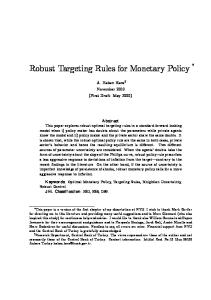
The staff uses the Taylor rule as a benchmark, which is compared to recent out-turns in the Bank’s base rate in Chart 1. Because there is little consensus in the academic literature on the appropriate cyclical response in the Taylor rule, the chart also provides a feel for the sensitivity of the rule to the output gap response. This is given by the shaded area, which varies the output gap response between 0.25 and 0.75.

Chart 1 Taylor Rule: quarterly (2001 Q4) Per cent 8.0

Nominal interest rate

7.0 6.0 5.0 4.0 3.0 T aylor rule

2.0 1.0 0.0

1993 1994 1995 1996 1997 1998 1999 2000 2001

Note: The shaded area describes the range of outcomes based on output gap weights between 0.25 and 0.75.

The Taylor rule’s prescriptions are also decomposed into contributions from inflation, the output gap and the equilibrium real interest rate (shown in Chart 2).

6

The equilibrium real interest rate is calculated by a statistical filter of the five-year real forward rate, five years forward, derived from the index linked yield curve.

9

Chart 2 Taylor Rule contributions

Levels (per cent) 10.0 8.0 6.0 4.0 2.0 0.0

Actual inflation Equilibrium real interest rate Inflation deviation from target Output gap measure

-2.0 -4.0

1993 1994 1995 1996 1997 1998 1999 2000 2001

When the rule’s prescriptions differ substantially from the Bank’s actual base rate, staff analyse the reasons for such deviations. For example, current inflation may rise due to temporary factors (such as a rise in seasonal food prices), generating an increase in the interest rate prescribed by the Taylor rule. But policy should not respond to such movements in relative prices unless they spill over into inflation expectations. Hence, in such circumstances, we would conclude that the Taylor rule is giving a misguided prescription.

The McCallum rule is of the following form: M = x* − vt −1 + 0.5( x* − xt −1 )

(1.2)

where M is the rule’s prescription for narrow money growth, x is actual nominal income growth, x* is target nominal income growth in steady state (assumed equal to 5%7), and v is trend velocity (a four quarter moving average of narrow money velocity). Again, similarly to the Taylor rule, Bank staff analyse recent changes in inflation and real GDP growth, as well as velocity trends. This provides a useful cross-check on interest rate rules since in theory interest rate and money supply rules should lead to similar outcomes provided that velocity is stable.8

7

This is based on an inflation target of 2.5% and an assumed trend annual real GDP growth of 2.5%.

10

Chart 3 McCallum Rule: quarterly (2001 Q3) Per cent 9.0 Actual M0 growth

8.0 7.0 6.0 5.0 4.0 3.0 2.0 1.0 0.0

1993 1994 1995 1996 1997 1998 1999 2000 2001

Note: The shaded area describes the range of outcomes based on nominal income growth rate gap weights between 0.25 and 0.75.

The Brainard rule gives a policy prescription when the policy-maker is uncertain about parameter values in his/her model of the economy. The Bank’s Brainard rule was derived by Martin and Salmon (1999) using a method first pioneered by Sack (1998) for the US. Its derivation uses a VAR with output, inflation, the short-term interest rate and the sterling effective exchange rate. The Brainard rule9 is used in much the same way as the Taylor rule. Staff comment on the terms that drive changes in the rule’s prescriptions, and compare the profile of the Bank’s repo rate to the path of rates suggested by the Brainard rule.

Bank staff also monitor a real interest rate gap measure derived by Neiss and Nelson (2001). It measures the difference between the actual real interest rate in the economy10 and a measure of the ‘neutral’ real interest rate – the real rate that would occur if prices were completely flexible. In other words, the gap measures whether the stance of policy is expansionary (current real rate is below ‘neutral’) or contractionary (current real rate is above ‘neutral’). However, the level of the real 8

Persistent differences between the McCallum rule’s prescriptions and actual money base growth in the absence of inflationary pressure could also indicate trend velocity shifts or changes in the economy’s trend growth rate.

9

The form of the rule is the following:

Rt = 0.109π t −1 + 0.99et + 47.545 yt −1 + 0.046π t −2 − 0.031et −1 − Rt −1 + 0.117 where e is the nominal exchange rate, and other variables are defined in the same way as the Taylor rule.

11

interest rate gap measure is dependent on an assumption about the long-term real interest rate and is therefore subject to considerable uncertainty. Bank staff concentrate on the changes in the measure to assess whether policy is becoming tighter or looser.

The Bank also uses a ‘reverse Taylor rule’ (calibrated with a coefficient of 1.5 on inflation and a coefficient of 1.0 on the output gap) to extract information on the market’s expectation of output growth from the short end of the yield curve11. The output growth forecasts from the reverse Taylor rule are then compared to Consensus Economics and internal forecasts of output growth.

So, to summarise, the Bank of England uses a number of monetary policy rules in its regular assessment of economic conditions and as part of forming its outlook for the prospects for inflation. Monetary policy rules and other measures of the policy stance are in effect a part of the Bank’s ‘suite of models’ approach to forecasting and economic assessment, whereby a number of different models are used to generate forecasts and answer policy questions. The policy prescriptions from each of the measures are carefully analysed in order to provide a robust assessment of the policy stance and the likelihood of future inflationary pressure. •

Monetary policy research

Bank staff use monetary policy rules in both estimated and calibrated macroeconomic models to inform thinking about issues of monetary strategy. Although the MPC does not use monetary rules in setting the policy rate, the academic literature on monetary

10

The inflation expectation in the model is computed using a VAR estimated on 1975-1999 quarterly UK data.

11

To see how this works, solve the standard Taylor rule in terms of the output gap term:

(

yt = yt* + Rt − rt ss − 1.5* π t − π *

)

So expected output growth in the next period is given by first differencing the above equation forward:

Et ∆yt +1 = g * + Et ∆Rt +1 − Et ∆rt ss+1 − 1.5* Et ∆π t +1 where g* is the potential output growth rate (assumed constant at 2.5% for the UK11),

Et ∆Rt +1 and

Et ∆π t +1 are, respectively, the slopes of the nominal yield curve and the slope of the inflation expectations term structure.

Et ∆rt ss+1 is the expected change in the equilibrium real interest rate, which

is assumed to be zero for simplicity.

12

policy rules can yield some important and interesting insights on how monetary policy should be conducted. King (1999) offers the following comment on the Taylor rule:

‘The idea that monetary policy does or should follow a Taylor rule has been extremely influential. Like most good ideas, its virtue is simplicity. It is not a mechanical rule to guide policy, but a vehicle to clarify issues.’

Many of the Bank’s research initiated in the monetary strategy area have examined what difference modifications to simple model set-ups make to the ‘rules’ which are then optimal. The insights gained may then illuminate the choice of policy strategy in more complex situations.

Batini and Haldane (1999) and Batini and Nelson (2000) examine the optimal horizon for inflation targeting. Both studies use standard calibrated small macroeconomic models to investigate the gains from forward-looking policy. The main conclusions of the papers are that forward-looking rules are optimal (in the sense of delivering the lowest sum of inflation and output volatility) when the underlying model of the economy is backward looking. The authors explain that by following a forwardlooking reaction function, the monetary authority can compensate for the inertial behaviour of the eocnomy.

Martin (1999) and Martin and Salmon (1999) investigate the extent to which the Brainard conservativism principle12 affects the prescriptions from an optimal monetary policy rule. They found that introducing parameter uncertainty generates more cautious behaviour than standard optimal rules. This is because policy makers are uncertain about the impact of interest rates on the economy and do not want to inject more variance into future outcomes. But, similarly to Sack (1998) for the US, the papers find that the resulting Brainard rules do not differ markedly from the optimal rules in the absence of uncertainty.

Bank staff have also carried out research on how optimal policy should respond to noisy indicators of economic conditions. This is a very important issue given the

12

The principle states that policy should be ‘cautious’ in the face of parameter uncertainty.

13

uncertainties brought about by large and frequent revisions to economic data. Aoki (2000) examines how optimal monetary policy should respond to noisy real-time data in a small macroeconomic model. He finds that the optimal rule involves a ‘cautious’ (quantitatively small) response to imperfectly measured indicators of economic conditions.

Batini and Yates (2001) examine how hybrid inflation and price level targeting rules (that incorporate both inflation and price level targeting terms) perform in a simple macroeconomic model. The authors find that such ‘hybrid rules’ give good performance in terms of output and inflation volatility while dramatically reducing the variance of the price level in forward looking models. But they conclude that any conclusions about the desirability of ‘hybrid rules’ are highly dependent on the modelling assumptions, and in particular, on the degree of forward-looking behaviour.

In the light of Japan’s experience over the last decade, the Bank has conducted research on the probability of hitting the zero lower bound on nominal interest rates. King (1999) conducts simulations with different monetary policy rules and examines the frequency of hitting the zero lower bound on nominal interest rates. He finds that aggressive (in the sense of having a large response coefficients to inflation and output) Taylor rules with lagged interest rate terms generate a high probability of hitting the zero nominal bound in backward-looking models, but small probabilities in forward-looking models. King explains that rules with lagged interest rate terms influence private sector behaviour more in forward-looking models because agents can foresee that a rise in interest rates is persistent. This allows the central bank to stabilise shocks with smaller variations of the nominal interest rate, making it less likely that nominal interest rates will reach zero.

The literature on monetary policy rules can also shed light on explanations for historical inflationary episodes. Following a growing US literature, Nelson and Nikolov (2001) have examined the extent to which mismeasurement of the output gap in real time may account for the monetary policy mistakes in the UK in the 1970s and late 1980s. They simulate a simple forward-looking macro-model with a Taylor rule and find that what in retrospect looks like a misjudgment of the output gap in real

14

time could account for a substantial proportion of the inflationary outbreak in the 1980s but a smaller proportion of the rise in inflation in the 1970s.

As the UK is a highly open economy, the Bank of England is interested in how economic openness changes the optimal design of monetary policy. Batini, Harrison and Millard (2001) have examined the performance of a number of rules in an optimising small open economy model calibrated to the UK. They find that Taylor rules perform badly, while forecast based rules that respond to a deviation of the inflation forecast from target give a robust performance. Adding exchange rate terms to simple monetary policy rules appears to improve performance although the gain is very small.

The 1990s have seen an increase in academic interest into the role of credit in economic fluctuations. Bean, Larsen and Nikolov (2002) examine this issue using a simple macroeconomic model, which is calibrated to match the behaviour of an economy with credit frictions. Using robust control techniques, the authors argue that credit frictions imply a more aggressive policy response in order to prevent persistent fluctuations in output and inflation.

4. Conclusions

The UK’s monetary policy arrangements combine a statutory commitment to low inflation with the discretion to respond to individual shocks as the MPC considers appropriate. Within the UK’s inflation targeting framework, mechanical monetary policy rules do not play a part in practical policy-making although they are used in economic assessment and research.

The Bank frequently reviews the prescriptions of common simple rules (such as the Taylor, McCallum and Brainard rules) as part of its ‘suite of models’ approach to assessment and forecasting. The tools of the monetary policy rules literature are also used actively to inform thinking about issues of monetary strategy.

15

References

Aoki, K. (2000), ‘Optimal indicators for monetary policy’, Princeton University mimeo.

Batini, N. and Haldane, A. (1999), ‘Forward-looking rules for monetary policy’, Bank of England Working Paper No. 91

Batini, N., Harrison, R. and Millard, S. (2001), ‘Monetary policy rules for an open economy’, Bank of England Working Paper No. 149.

Batini, N. and Nelson, E. (2000), ‘Optimal horizons for inflation targeting’, Bank of England Working Paper No. 119

Batini, N. and Yates, A. (2001), ‘Hybrid inflation and price level targeting’, Bank of England Working Paper No. 135

Bean, C., Larsen, J. and Nikolov, K. (2002), ‘Financial frictions and the monetary transmission mechanism: theory, evidence and policy implications’, ECB Working Paper No. 113

King, M. (1999), ‘Challenges for monetary policy: new and old’, prepared for the Symposium on “New Challenges for Monetary Policy” sponsored by the Federal Reserve Bank of Kansas City at Jackson Hole, Wyoming

King, M. (2001), Comment on L. Svensson, in The monetary transmission process: recent developments and lessons for Europe, Deutsche Bundesbank

Martin, B. (1999), ‘Caution and gradualism in monetary policy under uncertainty’, Bank of England Working Paper No. 105

Martin, B. and Salmon, C. (1999), ‘Should uncertain monetary policy-makers do less?’, Bank of England Working Paper No. 99

16

Neiss, K. and Nelson, E. (2001), ‘The real interest rate gap as an inflation indicator’, Bank of England Working Paper N0. 130

Nelson, E. and Nikolov, K. (2001), ‘UK inflation in the 1970s and 1980s: the role of output gap mismeasurement’, Bank of England Working Paper N0. 148

Sack, B. (1998), ‘Does the Fed Act Gradually? A VAR Analysis’, Federal Reserve Board of Governors FEDS Working Paper, No 17.

Svensson, L. (2001), ‘What is wrong with Taylor rules? Using judgment in monetary policy through targeting rules’, Princeton University mimeo.

Taylor, J. (1993), ‘Discretion versus policy rules in practice’, Carnegie-Rochester Conference Series on Public Policy, Vol. 39(1), pp. 195-214.

Taylor, J. (1999), ‘The monetary transmission mechanism and the evaluation of monetary policy rules’, Prepared for the Third Annual International Conference of the Central Bank of Chile on ‘Monetary Policy: Rules and Transmission Mechanisms,’ September 20-21, 1999.

Woodford, M. (2000), ‘Optimal monetary policy inertia’, NBER Working Paper No. 7261

17