DP2014-39

Moneta ry Policy, Incom plete Asset Ma rkets, and Welfare in a Small Open Economy Shigeto KITANO Kenya TAKAKU December 1, 2014

Monetary Policy, Incomplete Asset Markets, and Welfare in a Small Open Economy Shigeto Kitano∗

Kenya Takaku†

Abstract We develop a small open economy model with capital, sticky prices, and a simple form of financial frictions. We compare welfare levels under three alternative rules: a domestic inflation-based Taylor rule, a CPI inflation-based Taylor rule, and an exchange rate peg. We show that the superiority of an exchange rate peg over a domestic inflation-based Taylor rule becomes more pronounced under incomplete financial asset markets and more severe financial frictions.

Keywords: small open economy; DSGE; welfare comparison; incomplete financial market; Ramsey policy; exchange rate regime. JEL Classification: E42, E44, E52, F31, F41,G15.

∗

RIEB, Kobe University, 2-1, Rokkodai, Nada, Kobe, 657-8501 Japan, E-mail: [email protected]. Faculty of Business, Aichi Shukutoku University, 23, Sakuragaoka, Chikusa, Nagoya, 464-8671, Japan, E-mail: [email protected]. †

1

Introduction

The question of whether monetary policy in an open economy is fundamentally different from that in a closed economy is one of the most important policy issues in international macroeconomics. Pioneering studies in the literature of the New Keynesian open economy models, such as Clarida et al. (1998) and Gal´ı and Monacelli (2005), revealed that the policy problem in an open economy may be isomorphic to that in a closed economy. Their results suggest that policymakers in an open economy should respond solely to movements in domestic prices and that there is no role for exchange rate stabilization. However, the recent theoretical literature on the monetary policy in open economies emphasizes that there may be important cases against the above-mentioned classical view (Corsetti et al. (2010), Monacelli (2013)). One of the important deviations from the classical view is caused by asset market imperfection that prevents efficient international risk sharing. De Paoli (2009) has shown that when comparing complete and incomplete markets, the ranking of policy rules can be reversed depending on specific parameter values such as the elasticity of substitution between home and foreign produced goods. This study examines the impact of financial frictions on the desirability of monetary policy in an open economy. Specifically, the question posed is as follows: which is more appropriate for an economy with severe financial frictions: the pursuit of domestic price stability or exchange rate stability? Therefore, we specifically analyze the effect of debt elasticity of the country premium on the welfare level in a small open economy, which is not discussed by De Paoli (2009). This is because, as emphasized by Garcia-Cicco et al. (2010), the debt elasticity of the country premium can be interpreted as a reduced form of an economy’s financial frictions. We develop a small open economy model with capital, sticky prices, and the above-mentioned financial frictions. Thereafter, we analyze three alternative rules: a domestic inflation-based Taylor rule, a CPI inflation-based Taylor rule, and an exchange rate peg. Using the perturbation method presented by Schmitt-Groh´e and Uribe (2004), which computes second-order accurate solutions, and using the prevalent parameter values for calibration in the related literature, we measure conditional welfare levels on the condition of the calibrated steady state under the different policy rules. As a reference case, we apply a Ramsey-type analysis to obtain an optimal monetary policy. Thereafter, we obtain conditional welfare levels under the different policy rules and compare them to the reference case. We first confirm that a domestic inflation-based Taylor rule outperforms an exchange rate peg under complete asset markets. This result is consistent with previous studies in the literature (e.g., Gal´ı and Monacelli (2005)), which show that monetary policy in an open economy is isomorphic to that in a closed economy. We next show that in contrast, an exchange rate peg can outperform a domestic inflation-based Taylor rule under incomplete asset markets. This result of our analysis that policy ranking can be reversed depending on the configuration of asset markets is in line with that of De Paoli (2009). In the incomplete market case in which an exchange rate peg may outperform a domestic inflationbased Taylor rule, we find that as the debt elasticity of the country premium is higher, an exchange rate peg has significant superiority over a domestic inflation-based Taylor rule. In general, as financial frictions in an economy are more severe, the welfare level in an economy under any monetary policy regime will deteriorate. This is, indeed, the case in our study. However, as financial frictions in an economy are more severe under incomplete markets, the welfare level in an economy under a domestic inflation-based Taylor rule deteriorates further compared to that under an exchange rate peg. The intuition for this result of our analysis is straightforward, and well described by the argument of Corsetti et al. (2010) as follows: “...because of distortions resulting from incomplete markets, even if the exchange rate acts as a ‘shock absorber’ moving only in response to current and expected fundamentals, its adjustment does not necessarily contribute to achieving a desirable allocation. On the contrary, it may exacerbate misallocation of consumption...(line 14-18, page 868).” Since more severe financial frictions cause larger distortions, it may cause further deviations from a desirable allocation to pursue inward-looking targeting rules, which let the exchange rate act as a shock absorber. Consequently, the superiority of an exchange rate peg over a domestic inflation-based Taylor rule is more pronounced, 1

when financial frictions in an economy are more severe under incomplete markets. The policy implication of our study is immediate. The results of our study imply that when the economy’s financial market is less developed, the exchange rate peg regime may be more appropriate compared to the domestic inflation targeting regime.

2

The Model

We employ a standard sticky price, small open economy model. The model here is based on the small open economy structure developed by Gal´ı and Monacelli (2005) and Faia and Monacelli (2008), except that capital investment is included in our model. The world economy comprises a small open economy (home country) and the rest of the world (foreign country). Each economy is inhabited by a continuum of infinitely lived households and firms.

2.1

Households

A representative household maximizes its expected lifetime utility: E0

∞ ∑

{ β

t=0

t

} Ct1−σ Nt1+ϕ , − 1−σ 1+ϕ

(1)

where Ct denotes a composite consumption index in period t, and Nt denotes labor effort. Households consume differentiated goods produced by both domestic and foreign firms. The composite consumption index Ct is given by [ η−1 η−1 ] η 1 1 η−1 η η η Ct ≡ (1 − γ) CH,t + γ CF,tη , (2) where the parameter η(> 0) is the elasticity of substitution between domestic and foreign goods, and the parameter γ ∈ (0, 1) represents the degree of openness. CH,t and CF,t are the indices for the consumption of domestic and foreign goods, which are expressed by [∫

1

CH,t ≡

CH,t (j)

ε−1 ε

ε ] ε−1

dj

[∫ CF,t ≡

;

0

1

CF,t (j)

ε−1 ε

ε ] ε−1

dj

,

(3)

0

where ε(> 1) is the parameter for the elasticity of substitution among differentiated goods. The capital accumulation process is given as Kt+1 = (1 − δ)Kt + It −

ψK (Kt+1 − Kt )2 , 2

(4)

∫1 ε ε−1 where Kt stands for capital, It (≡ [ 0 It (j) ε dj] ε−1 ) is the investment expenditure for domestic investment goods, ψ K is the capital adjustment cost parameter, and δ is the depreciation rate of capital. 2.1.1

Complete market case

The household has access to domestic and international financial markets. Under complete markets, the household’s budget constraint is given as Pt Ct + PH,t It + Dt+1 + Et {dt,t+1 At+1 } = (1 + it−1 )Dt + At + Wt Nt + Rt Kt + ΠFt ,

(5)

∫1 1 1 1−η 1−η 1−η where Pt (≡ [(1−γ)PH,t +γPF,t ] ) denotes the consumer price index (CPI), PH,t (≡ [ 0 PH,t (j)1−ε dj] 1−ε ) ∫1 1 is the domestic price index, and PF,t (≡ [ 0 PF,t (j)1−ε dj] 1−ε ) is the import price index. Dt is the domestic bond, it is the nominal interest rate, At denotes the Arrow security traded in international financial markets, dt,t+1 is the stochastic discount factor for the Arrow security (in terms of domestic currency), Wt is the nominal wage, Rt is the rental rate of capital, and ΠFt denotes dividends from firms. 2

The optimality conditions associated with the household’s maximization problem are given by λt = Ct−σ , Ntφ , Wt /Pt { } λt+1 Pt 1 = β(1 + it )Et , λt Pt+1 λt =

and dt,t+1 = β

λt+1 Pt . λt Pt+1

(6) (7) (8)

(9)

The optimality condition associated with the Arrow security in the foreign country is given by dt,t+1 = β

λ∗t+1 Pt∗ Et , ∗ λ∗t Pt+1 Et+1

(10)

where the asterisk indicates foreign variables, and Et is the nominal exchange rate expressed as domestic currency per unit of foreign currency. Combining (9) and (10) and assuming symmetric initial conditions, we obtain 1 (11) Ct = Ct∗ Qtσ , where Qt (≡ condition. 2.1.2

Et Pt∗ ) Pt

denotes the real exchange rate. Equation (11) represents the international risk sharing

Incomplete market case

Under incomplete markets, the household’s budget constraint is given by Pt Ct + PH,t It + Dt+1 + Et Bt+1 = (1 + it−1 )Dt + (1 + ift−1 )Et Bt + Wt Nt + Rt Kt + ΠFt ,

(12)

where Bt denotes the foreign currency denominated bond traded in international financial markets, and ift denotes the domestic nominal interest rate on the bonds. The domestic interest rate ift is assumed to be the sum of the foreign nominal interest rate i∗t and a country premium that is increasing in the aggregate level of its foreign debt as follows: ( { } ) Et Bt EB f ∗ B it = it + ψ exp − + −1 , (13) Pt P where ψ B (> 0) is the parameter that governs the debt elasticity of the country premium. E, B, and P denote the steady state values of Et , Bt , and Pt , respectively. The optimality conditions associated with the domestic and foreign bonds are given by } { λt+1 Pt , (14) 1 = β(1 + it )Et λt Pt+1 {

and 1 = β(1 +

2.2

ift )Et

} λt+1 Pt Et+1 . λt Pt+1 Et

(15)

Firms

Firms operate in a monopolistic competitive market and produce differentiated goods. Each monopolistic firm j in the home economy produces a differentiated good with the following production function: Yt (j) = Zt Kt (j)α Nt (j)1−α ,

3

(16)

where Yt (j), Kt (j), Nt (j), and Zt denote the firm’s output, capital, labor inputs, and a stochastic productivity shock, respectively. The firm’s cost minimization implies that the firm’s real marginal cost is given by (Rt /PH,t )α (Wt /PH,t )1−α M Ct (j) = M Ct = . (17) Zt αα (1 − α)1−α Following Calvo (1983), we assume that in each period, a fraction 1 − ζ of firms reset their prices, whereas a fraction ζ keep their prices unchanged. Each firm chooses the price P¯H,t to maximize the present discounted value of its profit stream: max

∞ ∑

P¯H,t

n ζ k Et {Λt,t+k [Yt+k|t (P¯H,t − M Ct+k|t )]},

(18)

k=0

subject to Yt+k|t

( ¯ )−ε PH,t = Yt+k , PH,t+k

(19)

t where Λt,t+k (≡ β k ( CCt+k )−σ ( PPt+k )) denotes the discount factor, and Yt+k is the aggregate output level in t n period t + k. Yt+k|t and M Ct+k|t , respectively, denote the output level and the nominal marginal cost in t + k for a firm that last reset its price in period t. From the first-order condition associated with P¯ ) as follows: the above problem, we obtain the optimal price P˜H,t (≡ PH,t H,t

P˜H,t =

2.3

ε ε−1

{ ( )−ε−1 } PH,t k ζ E Λ Y M C t t,t+k PH,t+k t+k t+k|t k=0 . { ( ) } −ε ∑∞ k PH,t ζ E Λ Y t t,t+k PH,t+k t+k k=0

∑∞

(20)

Equilibrium and exogenous shocks

The market clearing condition for domestic goods is given by ∗ PH,t Yt = PH,t CH,t + PH,t It + PH,t CH,t ,

(21)

∗ where CH,t represents the foreign demand for domestic goods. Dividing both sides of (21) by PH,t yields ∗ Yt = CH,t + It + CH,t

= (1 − γ)g(St )η Ct + It + γStη Ct∗ ,

(22) 1

P

F,t ) denotes the terms of trade, and g(St )(≡ [(1 − γ) + γSt1−η ] 1−η ) denotes the ratio of the where St (≡ PH,t CPI (Pt ) to the domestic price index (PH,t ).1 Since a small open economy does not have any influence on the rest of the world, Ct∗ is assumed to be exogenous and equal to Yt∗ . The productivity shock Zt and the foreign output shock Yt∗ are assumed to exogenously evolve according to the following processes:

and

log Zt = (1 − ρz ) log Z + ρz log Zt−1 + εz,t , εz,t ∼ i.i.d. N (0, σz2 ),

(23)

2 ∗ ). + εy,t , εy,t ∼ i.i.d. N (0, σex log Yt∗ = (1 − ρy ) log Y ∗ + ρy log Yt−1

(24)

The second equality in (22) follows from the demand functions for the domestic goods: CH,t = (1 − γ) ( ∗ )−η P ∗ and CH,t = γ PH,t Ct∗ . ∗ 1

t

4

(

PH,t Pt

)−η

Ct ,

Table 1: Parameterization Parameters Value β σ φ ϵ ζ α ψK δ γ η ρz σz ρy σy ρz,y

2.4

0.99 2 3 6 0.75 0.32 15 0.025 0.28 1.5 0.66 0.0071 0.86 0.0078 0.3

Discount factor Inverse of intertemporal elasticity of substitution Inverse of Frisch elasticity of labor supply Elasticity of substitution among differentiated goods Fraction of firms that do not reset their prices Share of capital in output Capital adjustment cost parameter Depreciation rate of capital Degree of openness Elasticity of substitution between domestic and foreign goods Persistence: productivity shock Standard deviation: productivity shock Persistence: foreign output shock Standard deviation: foreign output shock Correlation between productivity shock and foreign output shock

Monetary policy rule

Following Gal´ı and Monacelli (2005), we consider the three alternative policy rules: a domestic inflationbased Taylor rule, a CPI inflation-based Taylor rule, and an exchange rate peg. The three policy rules are formalized as follows: ˜ H,t , ˜it = ϕΠ Π (25) ˜ t, ˜it = ϕΠ Π (26) and ∆Et = 1, (27) ( ) ˜ t ≡ Πt −Π denote the nominal interest rate, domestic in˜ H,t ≡ ΠH,t −ΠH , and Π where ˜it (≡ it − i) , Π ΠH Π ( ) Et flation, and CPI inflation deviations from their steady-state values, respectively. ∆Et ≡ Et−1 denotes the depreciation rate of the nominal exchange rate. (

2.5

)

Parameterization

We choose standard parameter values in the related literature for calibration, which are summarized in Table 1. Following many previous studies, we set the quarterly discount factor β, and the inverse of intertemporal elasticity of substitution σ to 0.99 and 2, respectively. Following Gal´ı and Monacelli (2005), we set the inverse of Frisch elasticity of labor supply φ, the elasticity of substitution among differentiated goods ϵ, and the fraction of firms that do not reset their prices ζ to 3, 6, and 0.75, respectively. We set the capital share in production α to 0.32 as in Schmitt-Groh´e and Uribe (2003). Following Kollmann (2002), we set the capital adjustment cost parameter ψ K and quarterly depreciation rate δ to 15 and 0.025, respectively. The degree of openness γ is set to 0.28 as in Cook (2004). Following Ravenna and Natalucci (2008), we set the elasticity of substitution between domestic and foreign goods η to 1.5. We use the same values as in the Gal´ı and Monacelli (2005) model for the exogenous shocks. The persistence and the standard deviation of the productivity shock (ρz and σz ) are set to 0.66 and 0.0071, respectively. The persistence and the standard deviation of the foreign output shock (ρy and σy ) are set to 0.86 and 0.0078, respectively. The correlation between the productivity shock and the foreign output shock ρz,y is set to 0.3. 5

3

Results

We calculate and compare welfare levels in the following cases: (a) a domestic inflation-based Taylor rule, (b) a CPI inflation-based Taylor rule, (c) an exchange rate peg, and (d) the Ramsey optimal policy.2 We let V0i denote the conditional welfare associated with the case (i) (i = a, b, c, d) on the condition of the calibrated steady state: V0i ≡ E0 = E0

∞ ∑ t=0 ∞ ∑

β t U (Cti , Nti ). (i = a, b, c, d) β t U ((1 − λi )C, N ).

(28)

t=0

Here, λi is the conditional welfare cost of adopting policy (i). The conditional welfare measure is obtained using second-order perturbation methods as described in Schmitt-Groh´e and Uribe (2004).3 Since the Ramsey optimal policy case (d) is the most welfare-maximizing, we let (d) be the reference case (ref ). Then, λi − λref denotes the welfare loss in each case, which is the fraction of consumption that compensates a household to a level that is considered as well off under the policy (i) as in the reference case (ref ).

3.1

Complete market case

First, we consider the case where the financial market is complete. Table 2 shows the conditional welfare losses associated with the three simple rules of a domestic inflation-based Taylor rule, a CPI inflationbased Taylor rule, and an exchange rate peg in the complete market case. DI Taylor, CPI Taylor, and Peg in Table 2 abbreviate the three rules, respectively. Similar to the model of Gal´ı and Monacelli (2005), we define the welfare loss in each case of DI Taylor, CPI Taylor, and Peg as deviations from the first best case, which is the Ramsey optimal case in our analysis. The results in Table 2 indicate that the welfare loss in the DI Taylor case is the smallest among the three simple rules, the CPI Taylor case is next to the DI Taylor case, and the welfare loss in the Peg case is the largest. Although our model differs from the model of Gal´ı and Monacelli (2005), wherein our model includes capital investment and we use the second-order perturbation method with the more plausible parameter values, we can confirm that the ranking of welfare is similar to that in the model of Gal´ı and Monacelli (2005). Table 2: Welfare Losses (%): complete market case Welfare losses DI Taylor CPI Taylor Peg

0.0430 0.0548 0.0572

Note) Letting the Ramsey policy case to be the reference case, we calculate the welfare loss in each case (i.e., λa − λref , λb − λref , λc − λref ).

3.2

Incomplete market case

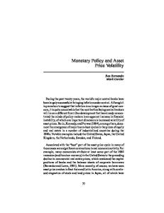
Next, we consider the incomplete market case. Figure 1 illustrates the welfare losses associated with the three simple rules of DI Taylor, CPI Taylor, and Peg in the incomplete market case. We calculate 2

We obtain the Ramsey optimal policy by setting up a Lagrangian problem in which the social planner maximizes the conditional lifetime utility of the representative household subject to the first-order conditions of the private agents and the market clearing conditions of the economy. We compute this numerically by using the Matlab procedures developed by Levin et al. (2006). 3 Kim and Kim (2003) reveal that second-order solutions are necessary because conventional linearization may generate spurious welfare reversals.

6

welfare losses associated with a wide range of values for the parameter governing the debt elasticity of the country premium ψB from 0.05 up to 3. As is well known, we must avoid the case where ψB is zero to induce stationarity (Schmitt-Groh´e and Uribe (2003)). The range of ψB is chosen because Garcia-Cicco et al. (2010) estimate ψB at 2.8 from Argentine’s economy’s data, and suggest that the parameter value of the debt elasticity of the country premium for emerging market economies is higher than that for developed countries. Since the parameter value of ψB for emerging market economies is high, Figure 1 implies that the superiority of Peg compared to DI Taylor (and CPI Taylor) would be relevant for emerging market economies. In addition, Figure 1 illustrates that as the parameter value of ψB increases, the difference between the welfare loss in the Peg case and those in the other two cases of DI Taylor and CPI Taylor expands. Garcia-Cicco et al. (2010) argue that ψB is the critical parameter in replicating the emerging market economies, and that this parameter can be interpreted as a reduced form that captures the degree of an economy’s financial frictions. That is, the higher value of ψB means that an economy’s financial frictions are more severe. Therefore, in general, as financial frictions in an economy are more severe, the welfare level in an economy under any monetary rules will deteriorate. This is the case in our study. However, as illustrated in Figure 1, as financial frictions in an economy are more severe under incomplete markets, the welfare level in an economy in the DI Taylor case deteriorates further compared to that in the Peg case. This is because, as argued by Corsetti et al. (2010), when an economy is under incomplete markets and the flexibility of exchange rate does not necessarily contribute toward achieving a desirable allocation, it may not be optimal to pursue inward-looking targeting rules such as DI Taylor, which let the exchange rate act as a shock absorber. Rather, the inward-looking targeting rules such as DI Taylor may exacerbate misallocation. As the financial frictions in an economy are more severe, the distortions resulting from incomplete markets are larger. Consequently, the welfare in the DI Taylor case deteriorates further than the Peg case, and the superiority of the Peg case over the DI Taylor case is more pronounced.

7

Figure 1: Welfare losses (%): incomplete market case 0.085

DI Taylor CPI Taylor PEG

0.08

0.075

Welfare losses (%)

0.07

0.065

0.06

0.055

0.05

0.045

0.04

0

0.5

1

1.5 ψB

2

2.5

3

Note) Letting the Ramsey policy case to be the reference case, we calculate the welfare loss in each case. (i.e., λa − λref , λb − λref , λc − λref )

8

4

Conclusion

We develop a small open economy model with capital, sticky prices, and a simple form of financial frictions a la Garcia-Cicco et al. (2010). Considering the Ramsey optimal policy as the reference case, we calculate the conditional expected lifetime utility of the representative household and obtain the conditional welfare losses under three alternative rules: a domestic inflation-based Taylor rule, a CPI inflation-based Taylor rule, and an exchange rate peg. First, we confirm that a domestic inflation-based Taylor rule is the best and an exchange rate peg is the worst in the ranking of the conditional welfare losses under complete financial asset markets. This result is in line with the previous studies with complete markets such as those by Gal´ı and Monacelli (2005). In contrast, we show that an exchange rate peg is more superior to a domestic inflation-based Taylor rule and a CPI inflation-based Taylor rule under incomplete asset markets and more severe financial frictions. The result of our analysis that policy ranking can be reversed depending on the configuration of asset markets is in line with that of De Paoli (2009). However, we specifically analyze the effect of debt elasticity of the country premium on the welfare level in a small open economy, which is not discussed by De Paoli (2009). As emphasized by Garcia-Cicco et al. (2010), the debt elasticity of the country premium can be interpreted as a reduced form of an economy’s financial frictions. We have examined the impact of financial frictions on the desirability of monetary policy in a small open economy. Specifically, we contribute to the literature by showing that the superiority of an exchange rate peg over a domestic inflation-based Taylor rule is more evident as an economy’s financial frictions are more severe. Since the financial frictions of emerging market economies are quite severe as suggested by the previous studies, the result of our analysis implies that it might not be appropriate for policy makers in emerging market economies to ignore exchange rate stability.

References Calvo, Guillermo A. (1983) “Staggered Prices in a Utility-Maximizing Framework,” Journal of Monetary Economics, Vol. 12, No. 3, pp. 383 - 398. Clarida, Richard, Jordi Gali, and Mark Gertler (1998) “Monetary Policy Rules in Practice Some International Evidence,” European Economic Review, Vol. 42, No. 6, pp. 1033-1067. Cook, David (2004) “Monetary Policy in Emerging Markets: Can Liability Dollarization Explain Contractionary Devaluations?” Journal of Monetary Economics, Vol. 51, No. 6, pp. 1155 - 1181. Corsetti, Giancarlo, Luca Dedola, and Sylvain Leduc (2010) “Optimal Monetary Policy in Open Economies,” in Friedman, Benjamin M. and Michael Woodford eds. Handbook of Monetary Economics, Vol. 3: Elsevier, Chap. 16, pp. 861-933. De Paoli, Bianca (2009) “Monetary Policy under Alternative Asset Market Structures: The Case of a Small Open Economy,” Journal of Money, Credit and Banking, Vol. 41, No. 7, pp. 1301–1330. Faia, Ester and Tommaso Monacelli (2008) “Optimal Monetary Policy in a Small Open Economy with Home Bias,” Journal of Money, Credit and Banking, Vol. 40, No. 4, pp. 721–750. Gal´ı, Jordi and Tommaso Monacelli (2005) “Monetary Policy and Exchange Rate Volatility in a Small Open Economy,” Review of Economic Studies, Vol. 72, No. 3, pp. 707-734. Garcia-Cicco, Javier, Roberto Pancrazi, and Martin Uribe (2010) “Real Business Cycles in Emerging Countries?” American Economic Review, Vol. 100, No. 5, pp. 2510-31. Kim, Jinill and Sunghyun Henry Kim (2003) “Spurious Welfare Reversals in International Business Cycle Models,” Journal of International Economics, Vol. 60, No. 2, pp. 471-500.

9

Kollmann, Robert (2002) “Monetary Policy Rules in the Open Economy: Effects on Welfare and Business Cycles,” Journal of Monetary Economics, Vol. 49, No. 5, pp. 989-1015. Levin, Andrew T., Alexei Onatski, John Williams, and Noah M. Williams (2006) “Monetary Policy under Uncertainty in Micro-Founded Macroeconometric Models,” in Gertler, Mark and Kenneth Rogoff eds. NBER Macroeconomics Annual 2005, Volume 20: MIT Press, pp. 229-312. Monacelli, Tommaso (2013) “Is Monetary Policy in an Open Economy Fundamentally Different?” IMF Economic Review, Vol. 61, No. 1, pp. 6 - 21. Ravenna, Federico and Fabio M. Natalucci (2008) “Monetary Policy Choices in Emerging Market Economies: The Case of High Productivity Growth,” Journal of Money, Credit and Banking, Vol. 40, No. 2-3, pp. 243-271. Schmitt-Groh´e, Stephanie and Martin Uribe (2003) “Closing Small Open Economy Models,” Journal of International Economics, Vol. 61, No. 1, pp. 163 - 185. Schmitt-Groh´e, Stephanie and Mart´ın Uribe (2004) “Solving Dynamic General Equilibrium Models Using a Second-Order Approximation to the Policy Function,” Journal of Economic Dynamics and Control, Vol. 28, No. 4, pp. 755 - 775.

10