Int. J. Monetary Economics and Finance, Vol. 7, No. 3, 2014

Monetary policy and oil price fluctuations following the subprime mortgage crisis Naoyuki Yoshino Asian Development Bank Institute, Kasumigaseki Building 8F, 3-2-5 Kasumigaseki, Chiyoda-ku, Tokyo 100-6008, Japan E-mail: [email protected] E-mail: [email protected]

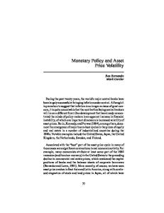
Farhad Taghizadeh-Hesary* Economics Department, Keio University, 2-15-45 Mita, Minato-ku, Tokyo 108-8345, Japan and Institute of Energy Economics, Japan (IEEJ), 1-13-1, Kachidoki, Chuo-ku, Tokyo 104-0054, Japan E-mail: [email protected] E-mail: [email protected] *Corresponding author Abstract: This study examines how monetary policy affected crude oil prices after the subprime mortgage crisis. Our earlier research found that easy monetary policy had a significant impact on energy prices during the period of 1980–2011. This paper finds that after the subprime mortgage crisis the weaker exchange rate of the US dollar caused by the country’s quantitative easing pushed oil prices in US dollars upward over the period of 2009–2012, by causing investors to invest in the oil market and other commodity markets while the world economy was in recession in this period. This trend had the effect of imposing a longer recovery time on the global economy, as oil has been shown to be one of the most important production inputs. Keywords: oil prices; monetary policies; subprime mortgage crisis; exchange rate. Reference to this paper should be made as follows: Yoshino, N. and Taghizadeh-Hesary, F. (2014) ‘Monetary policy and oil price fluctuations following the subprime mortgage crisis’, Int. J. Monetary Economics and Finance, Vol. 7, No. 3, pp.157–174. Biographical notes: Naoyuki Yoshino is the Dean of the Asian Development Bank Institute (ADBI) and Professor Emeritus at Keio University, Japan. He obtained his PhD from Johns Hopkins University, USA, in 1979. His professional career includes membership in numerous government committees. He was a visiting scholar at the Central Bank of Japan from 1994 to 1995.

Copyright © 2014 Inderscience Enterprises Ltd.

157

158

N. Yoshino and F. Taghizadeh-Hesary He was named Director of the Japan Financial Services Agency’s (FSA) Financial Research Center (FSA Institute) of the Government of Japan in 2004 and is now Chief Adviser. He obtained his honorary doctorates from the University of Gothenburg (Sweden) in 2004 and Martin Luther University of Halle-Wittenberg (Germany) in 2013. He also received the Fukuzawa Award in 2013 for his contribution to research on economic policy. Farhad Taghizadeh-Hesary is a Researcher of Economics at the School of Economics, Keio University, Japan. He is also serving as a visiting scholar at the Institute of Energy Economics of Japan (IEEJ). He is pursuing his PhD at the Graduate School of Economics, Keio University, under the supervision of Professor Naoyuki Yoshino, and also assists Professor Yoshino in his capacity as the Dean of the Asian Development Bank Institute. His major research interests lie in the areas of energy economics, monetary economics, banking, deposit insurance and financing of SMEs.

1

Introduction

The subprime mortgage crisis began when the US housing bubble burst and sparked a global financial crisis in 2007 and 2008. Before the crisis, over a period of several years, housing prices had been increasing while interest rates remained low. Subprime mortgages were extensively available and refinancing was cheap. However, as interest rates increased and housing prices started to drop owing to the huge housing supply, refinancing became more difficult and the risks embedded in subprime mortgages could no longer be hidden. In August 2007, these problems hit the global financial markets and caused enormous liquidity pressures within the interbank market. Because of the widespread dispersion of credit risk and the complexity of financial instruments, the mortgage crisis had a large impact on financial markets. In July 2007, stock market indices began to see massive declines. Several large banks, and credit insurance and mortgage companies reported significant losses and dropped much of their market value. Because of this drop in global output and a reluctance to borrow from banks, commodity markets, including crude oil market demand, also experienced sharp drops and subsequently large price decreases. In the USA, the Federal Reserve (Fed) held between $700 and $800 billion worth of Treasury notes on its balance sheet before the recession. To mitigate some of the adverse effects of the crisis, in late November 2008 it began to purchase $600 billion in mortgage-backed securities. By March 2009, it held $1.75 trillion worth of bank debt, mortgage-backed securities and Treasury notes, reaching a peak of $2.1 trillion in June 2010. Further purchases were halted as the economy began to improve, but resumed in August 2010 when the Fed decided that the economy was not growing robustly enough. After the halt in June, holdings started to fall naturally as debt matured, and were projected to fall to $1.7 trillion by 2012. The Fed’s revised goal became to keep holdings at $2.054 trillion. To maintain this level, the Fed bought $30 billion in 2–10-year Treasury notes every month. In November 2010, the Fed announced a second round of quantitative easing, buying $600 billion of Treasury securities by the end of the Q2 2011. ‘QE2’ became a ubiquitous nickname in 2010, used to refer to this second round of quantitative easing by US central banks (Authers, 2010). Retrospectively, the round of quantitative easing preceding QE2 was called ‘QE1’ (Conerly, 2012). A third round of

Monetary policy and oil price fluctuations

159

quantitative easing, ‘QE3’, was announced on 13 September, 2012. Additionally, the Federal Open Market Committee (FOMC) announced that it would likely maintain the federal funds rate near zero at least through 2015. According to the International Monetary Fund (IMF), quantitative easing policies that were undertaken by the central banks of the major developed countries, as in the example of the US quantitative easing policies mentioned earlier, have contributed to a reduction in systemic risk following the crisis. The IMF states that these policies also contributed to improvements in market confidence and the bottoming out of the recession in the Group of 7 (G7) economies in the second half of 2009 (Klyuev et al., 2009). However, there are several economists, such as Ratti and Vespignani (2013), who concluded that quantitative easing undertaken by the central banks of different countries following the 2007–2008 crisis played a large role in the fast recovery of commodity prices, especially with regard to the oil market. This trend had the effect of imposing a longer recovery time on the economy, as the oil has been shown to be one of the most important production inputs. This means that increasing oil prices are destructive for economic growth and tend to prolong economic recovery time. The hypothesis of this paper is in line with the latter paper because we believe that quantitative easing policies undertaken by central banks in the USA and other countries following the economic crisis rapidly pushed up commodity market prices. This rise includes crude oil prices, which caused a longer recovery time for the global economy. Figure 1 shows movements during the period January 2007–October 2013 of the interest rate (US money market rate) and the crude oil price (simple average of the Dubai, Brent and West Texas Intermediate (WTI) crude oil prices in constant dollars). Expansionary monetary policy in the USA led to a decrease in the US money market rate from 5.25% per annum in January 2007 to 2% per annum in June 2008. During the same period, crude oil prices saw an increase from around $53.35/barrel to beyond $131.70/barrel. We believe that a major cause of these skyrocketing prices was easy monetary policy. Figure 1

Interest rates and crude oil prices, January 2007–October 2013

Crude oil prices (right-hand scale) are in constant dollars obtained using the simple average of: Dubai crude oil prices in the Tokyo market, Brent crude oil prices in the London market and West Texas Intermediate (WTI) crude oil prices in the New York market, deflated by the US consumer price index (CPI). Interest rates (left-hand scale) are the US money market rate, percent per annum.

160

N. Yoshino and F. Taghizadeh-Hesary

Following the financial crisis of 2007–2008, a decline in global demand for crude oil caused oil prices to drop from $133.11 in July 2008 to below $42.01 in December 2008. After this dip, prices started to increase again. A portion of this elevation was due to increased demand stemming from a recovery in the global economy that increased demand, but we believe a significant reason for this sharp rise was the quantitative easing implemented by the monetary authorities. This easy monetary policy led to an elevation in crude oil demand, causing oil prices to increase rapidly. The result was that in May 2009, although the global economy had not recovered completely, crude oil prices almost surpassed their pre-crisis levels of January 2007. In this paper, we answer to the question of whether monetary policy had a significant impact on the crude oil market following the subprime mortgage crisis. This paper is structured as follows. In the following section, we review the literature. Section 3 details the theoretical background and the model, including: Section 3.1, monetary policy transmission channels to oil demand; Section 3.2, the effect of monetary policy actions on exchange rates; Section 3.3, definition of the real effective exchange rate (REER); Section 3.4, the theoretical framework and Section 3.5, the model. Section 4 describes the empirical results, including: Section 4.1, data analysis; Section 4.2, structural parameter estimates and Section 4.3, structural impulse response (IR) analysis. Section 5 contains the concluding remarks.

2

Review of the literature

In the literature on energy economics, there are several research cases that have found a significant impact of monetary policy on energy markets, especially the crude oil market. Barsky and Kilian (2002) argued that changes in monetary policy regimes were a key factor behind the oil price increases of the 1970s, and show that the substantial increase in industrial commodity prices that preceded the increase in oil prices (1973–1974) is consistent with the view that rising demand based on increased global liquidity drove oil prices higher. Additionally, a more recent study by Taghizadeh and Yoshino (2014) demonstrated that global oil demand during the periods 1960–2011 and 1980–2011 was significantly influenced by monetary policy regimes. They showed that aggressive monetary policy stimulates oil demand, while supply remains inelastic to interest rates. The result is skyrocketing crude oil prices, which have the effect of inhibiting economic growth. On the other hand, Bernanke et al. (1997) showed that expansionary monetary policy could have largely eliminated the negative output consequences of the oil price shocks on the US economy. This view has, in turn, also been challenged by Hamilton and Herrera (2004), who argue that Bernanke, Gertler and Watson’s (BGW) empirical results suffer from model misspecification. Hamilton and Herrera reproduced the BGW experiment using a different model specification, and found that increases in the price of oil lead directly to contractions in real output. The tightening of monetary policy in the period that BGW examined played only a secondary role in generating the downturn. There are several other recent studies that critically reevaluate the results of Bernanke et al. (1997). For example, Leduc and Sill (2004) examined the Fed’s behaviour starting in 1979, and showed that monetary policy contributed to an approximate 40% drop in output following the rise in oil prices. The hypothesis of this paper is in agreement with

Monetary policy and oil price fluctuations

161

Barsky and Kilian (2002), Leduc and Sill (2004), Hamilton and Herrera (2004), Askari and Krichene (2010), Kormilitsina (2011), Ratti and Vespignani (2013), and Taghizadeh and Yoshino (2013a, 2013b, 2014) findings for the impact of monetary policy on crude oil prices. However, the main innovation of this paper is that we will test another channel of monetary policy transmission, the exchange rate.

3

Theoretical background and the model

3.1 Channels of transmission of monetary policy to oil demand Monetary policy affects oil demand through a number of channels, including interest rates and exchange rates. Channels of interest rate transmission could be completely described by classical monetarism, as well as in modern literature such as the Keynesian IS-LM model. Easing interest rates increases the demand for credit and increases aggregate demand, which includes the demand for commodities. This increased demand for commodities includes demand for energy, especially for crude oil and its derivatives because they are major energy carriers (Taghizadeh and Yoshino, 2014). Keynes (1936) examined the effects that lowered interest rates have on aggregate demand: expansionary monetary policy reduces the interest rate, and when the interest rate is lower than the marginal productivity of capital, it broadens investment demand until the marginal productivity of capital is equalised to a lower interest rate (Yoshino and TaghizadehHesary, 2014a). This expansion of investment creates an accelerator-multiplier effect, causing aggregate demand to expand, which in turn amplifies demand for commodities and puts pressure on commodity prices. This can be generalised for energy carriers as well, especially crude oil. In the end, this process leads to increased pressure on oil prices. In other words, lower interest rates make borrowing cheaper, which increases demand in the commodities market, including the crude oil market. As for the exchange rate transmission channel, most oil sales throughout the world are denominated in US dollars. This means that a depreciation of the US dollar makes oil imports cheaper in non-dollar-denominated currencies, raising oil imports and oil demand. Another exchange rate channel is that depreciation of the US dollar causes an appreciation of non-dollar-denominated financial assets. The majority of world financial assets are denominated in non-dollar currencies, so a depreciation of the US dollar stimulates world oil demand through the wealth effect. Figure 2 shows the REER and real crude oil price movements during the period January 2007–September 2013. The inverse relationship between these two variables is apparent in this figure. Generally, crude oil prices began to rise following depreciation of the US dollar, and dropped following an appreciation (For more information on the impact of exchange rate fluctuations on crude oil prices, see Reboredo (2012), Taghizadeh and Yoshino (2014) and Brahmasrene et al. (2014)). Another way to verify our hypothesis can be seen in Figure 3. Figure 3 illustrates the base money growth rate trend and the crude oil price movements during the period of February 2007–September 2013. As it is clear, in most cases they tend to follow the same path.

162 Figure 2

N. Yoshino and F. Taghizadeh-Hesary Exchange rate and crude oil prices, January 2007–September 2013

REER = real effective exchange rate. Crude oil prices (right-hand scale) are in constant dollars obtained using simple average of: Dubai crude oil prices in the Tokyo market, Brent crude oil prices in the London market and WTI crude oil prices in the New York market, deflated by the US consumer price index (CPI). REER (left-hand scale) is for the US dollar. Source: International Energy Agency (IEA) (2013); International Financial Statistics (IFS) (2013); The Energy Data and Modelling Centre (EDMC) database of the Institute of Energy Economics, Japan (IEEJ) Figure 3

Base money and crude oil prices, February 2007–September 2013

Crude oil prices (left-hand scale) are in constant dollars obtained using a simple average of: Dubai crude oil prices in the Tokyo market, Brent crude oil prices in the London market and WTI crude oil prices in the New York market, deflated by the US consumer price index (CPI). The base money growth rate (right-hand scale) is for the US dollar, seasonally adjusted.

Monetary policy and oil price fluctuations

163

3.2 The effect of monetary policy actions on exchange rates The effect of monetary policy on exchange rates has been the subject of a large body of empirical research since the early 1990s. This research includes: Sims (1992), Clarida and Gali (1994), Eichenbaum and Evans (1995), Bonser-Neal et al. (1998), Bagliano and Favero (1999), Bitzenis and Marangos (2007), and Bahmani and Bahmani-Oskooee (2012). Several of these empirical studies found that a tightening of US monetary policy is associated with an appreciation of the US dollar, while a loosening is associated with dollar depreciation. Using VAR methodology, Eichenbaum and Evans (1995) find that contractionary shocks to monthly values of the federal funds rate, the ratio of non-borrowed reserves to total reserves, and the Romer and Romer (1989) index over the period 1974–1990 led to a sharp increase in the differential between US and foreign interest rates, as well as to a sharp appreciation in the US dollar. Clarida and Gali (1994), Evans (1994) and Lewis (1995) used similar methods to find that contractionary US monetary policy is associated with dollar appreciation. Bonser-Neal et al. (1998) found that increases in the federal funds rate target during the periods 1974–1979 and 1987–1994, which targeted interest rates, are associated with significant increases in the value of the dollar. Zettelmeyer (2004) studied the impact effect of monetary policy shocks on the exchange rates of three small open economies (Australia, Canada and New Zealand) during the 1990s. The study found that a 100 basis point contractionary shock will force the exchange rate to appreciate by 2–3% on impact. The association of interest rate hikes with depreciations that can sometimes be observed during periods of exchange market pressure is mainly attributable to reverse causality. While all of these studies estimate US dollar appreciation in response to contractionary monetary policy shocks, they report a different dynamic response pattern. Bonser-Neal et al. (1998), for example, estimate spot and forward rate responses consistent with standard overshooting models in the majority of the cases they examine. In contrast, Clarida and Gali (1994), Eichenbaum and Evans (1995) and Evans (1994) estimate that it can take from 1 to 3 years for the maximal effect of the policy shock to be felt on exchange rates. Bonser-Neal et al. (1998) also estimate that the impact of a policy shock is expected to increase over time, as in the case of the yen/US dollar exchange rate over the period 1974–1979. These latter results are clearly inconsistent with standard overshooting models. In overshooting models, contractionary US monetary policy causes the US dollar spot rate to temporarily appreciate beyond, or overshoot, its new higher equilibrium level. Future exchange rates are, therefore, expected to appreciate by less than the current spot rate in response to a tightening of monetary policy. Bonser-Neal et al. (2000) suggest that the standard overshooting model may be too restrictive to completely characterise the effects of monetary policy on exchange rates.

3.3 Definition of the real effective exchange rate (REER) The relative attractiveness of domestic goods compared with foreign goods depends primarily on their relative price. We can think of this relative price as the number of domestic goods that must be given up to acquire one foreign good. This relative price is called the ‘real exchange rate.’ This real exchange rate can be expressed in both bilateral and multilateral (or effective) terms. The multilateral real exchange rate (or the REER – the two terms are synonymous and are both in common use) is constructed from bilateral

164

N. Yoshino and F. Taghizadeh-Hesary

real exchange rates. It is simply the geometrically weighted average of the relevant set of bilateral real exchange rates. Note that a country’s nominal and real exchange rates do not have to move in the same direction. Figure 4 shows that the REER and nominal effective exchange rate (NEER) do not necessarily follow the same path. As can be seen from the definition of the real exchange rate, changes in the bilateral real exchange rate depend on two different factors: changes in the nominal exchange rate and changes in a country’s price level relative to that of its trading partner. For example, in many developing countries that experienced high inflation during the 1980s and 1990s, it was not at all uncommon for their bilateral real exchange rates against the US dollar to appreciate significantly, while their nominal exchange rates were depreciating (Montiel, 2009), simply because their domestic inflation rates were so much higher than the inflation rate in the USA. Figure 4

Nominal effective exchange rate (NEER) and real effective exchange rate (REER) for the US Dollar, 1980–2011

Both are consumer price index exchange rates (2005 = 100). Source: International Financial Statistics (IFS) (2013)

Effective exchange rate indices are constructed in three steps. First, the relevant bilateral exchange rates for a particular county are converted into indexes, using a common base year. Next, a set of weights is chosen to be applied to each of the bilateral indexes. Finally, the bilateral indexes are averaged together using these weights. While this may seem straightforward, there are several issues that have to be taken into consideration, such as geometric or arithmetic weighting, choice of weights, number of currencies and the base year for weights.

3.4 Theoretical framework In developing the theoretical framework of this paper, we used Taghizadeh and Yoshino (2014) for inspiration. Our assumed oil importing country/region has a multi-input production function, with four production inputs: yt = f ( K t , N t , q1dt , q2dt )

(1)

Monetary policy and oil price fluctuations

165

where yt is the total production (the monetary value of all goods produced in a year; gross domestic product (GDP)), K t is the capital input (the monetary worth of all machinery equipment and buildings), Nt is the labour input (the total number of manhours worked in a year), q1dt is the crude oil input (in barrels) and q2dt is the natural gas input (in cubic feet). An oil importer’s profit equation is: Max π td = Pyt . yt − it K t − wt N t − et p1t q1dt − et p2t q2dt

(2)

where Pyt is the output price level, wt is the labour wage, it is the borrowed capital rent, p1t is the crude oil price in US dollars, p2t is the natural gas price in US dollars, and et is the exchange rate. The Lagrange function is defined as:

L = ( Pyt yt − it K t − wt N t − et p1t q1dt − et p2t q2dt ) − λ  yt − f ( K t , N t , q1dt , q2dt ) 

(3)

This produces the first-order condition for crude oil: ∂L ∂q1dt = −  et p1t + ( ∂p1t ∂q1dt ) .et q1dt  + Pyt ( ∂f ∂q1dt ) = 0

(4)

More specific results can be obtained by adopting the Cobb-Douglas production function: yt = f ( K t , N t , q1dt , q2dt ) = bt K t α N t β ( q1dt )

γ1

(q )

d γ2 2t

(5)

where α, β , γ 1 , γ 2 are the output elasticities of capital, labour, crude oil and natural gas, respectively. These values are constants determined by available technology, and b is the total factor productivity. We have assumed that capital comes from the competitive market and that the crude oil market is oligopolistic. For information regarding oligopolistic markets, we referred to Revankar and Yoshino (2008). By rewriting equation (4), accounting for our Cobb-Douglas production function, we get: −  et p1t + ( ∂p1t ∂q1dt ) .et q1dt  + Pyt γ 1 ( yt q1dt ) = 0

(6)

To show that capital and labour inputs are functions of these variables, we rewrite equation (5) as follows: yt = bt K t α (it , yt ) N t β ( Pytt w

, yt )

(q ) (q ) d γ1 1t

d γ2 2t

(7)

and as we know: qitd = f ( pit Pyt ); (i = 1, 2)

(8)

For estimation purposes, we can express the oil demand function in simplified log-linear form as follows:1 q1dt = d 0 + d1 p1t + d 2 p2t + d3 yt + d 4 it + d5 et + udt

(9)

where q1dt is the logarithm of q1dt , pit is the logarithm of ( pit / p yt ); (i = 1, 2) , the coefficient d1is the price elasticity of crude oil demand and d2 is the substitution elasticity of natural gas, which is the main substitution for crude oil. To demonstrate the effect of changes in economic activity on the demand for oil, we use the real GDP in logarithmic form: ( yt = log( yt / Pyt ) ) . We also include two monetary policy factors: real interest rate

166

N. Yoshino and F. Taghizadeh-Hesary

( it ) and REER ( et ) . We expect negative values for both d4 and the exchange rate coefficient (d5), implying that a depreciation of the US dollar would increase demand for oil. d0 is the constant demand and udt is the random error term. We can write the crude oil price equation as follows: p1t = µ0 + µ1 Dtexcess + µ 2 p2t + µ3 yt + µ 4 it + µ5 et + u pt

(10)

where Dtexcess = q~1dt − q~1st denotes the excess demand in the crude oil market, which was obtained by deducting the crude oil supply from its demand. µi ; (i = 1,..., 5) are the coefficients of variables in crude oil price equation, µ0 is the constant and u pt is the random error term.

3.5 The model The objective of this section is to examine the relationship between crude oil prices, natural gas prices, REER, GDP and excess demand.2 To assess this relationship, we adopt the K variable structural vector autoregression (SVAR) as in Sims (1980), and start with the following VAR model: Yt = A1Yt −1 +

+ ApYt − p + ut

(11)

where Yt is a (K × 1) vector of variables and is comprised et , yt , p2t , Dtexcess , p1t Ai (i = 1,… , p) are (K × K ) fixed coefficient matrices, p is the order of VAR model and ut is a (K × 1) vector of VAR observed residuals with a zero mean and covariance matrix E ( ut ut′ ) = ∑ u . The innovations of the reduced form model ut can be expressed as a linear combination of the structural shock ε t as in Breitung et al. (2004) and Narayan (2013): ut = A−1 Bε t

(12)

where B is a structural form parameter matrix. Substituting equation (12) into equation (11), and following minor operations, we obtain the following, which is the structural representation of equation (11): AYt = A1*Yt −1 +

+ A*pYt − p + Bε t

(13)

where A*j ( j = 1,… , p) is a (K × K ) matrix of coefficients in which −1 * Aj = A Aj ( j = 1,… , p ) and ε t is a (K × 1) vector of unobserved structural shocks, with ε t ~ (0 ,I k ) . The structural innovation is orthonormal, that is, the structural covariance matrix, ∑ = E (ε t ε tt′ ) , IK is the identification matrix. This model is known as the AB ε model, and is estimated in the following form: Aut = Bε t

(14)

The orthonormal innovation ε t ensures the identifying restrictions on A and B: A∑ A′ = BB ′

(15)

Monetary policy and oil price fluctuations

167

Both sides of the expression are symmetric, which means that K (K + 1) / 2 restrictions need to be imposed on 2K 2 unknown elements in A and B. At least, 2 K 2 − K ( K + 1) / 2 additional identifying restrictions are needed to identify A and B. Considering the five endogenous variables that we have in our model, et , yt , p2t , Dtexcess , p1t , the errors of the reduced form VAR are: ut = ute + uty + utp2 + utDexcess + utp1 . The structural disturbances, ε te , ε ty , ε tp2 , ε tDexcess , ε tp1 , are the REER of the US dollar, real GDP of all Organisation of Economic Cooperation and Development (OECD) economies, natural gas real prices, excess demand in the world crude oil market and crude oil real price shocks, respectively.3 This model has a total of 50 unknown elements, and a maximum number of 15 parameters can be identified in this system. Therefore, at least 35 additional identifiable restrictions are required to identify matrices A and B. The elements of the matrices that are estimated have been assigned arc. All the other values in the A and B matrices are held fixed at specific values. Since this model is over-identified, a formal likelihood ratio (LR) test needs to be carried out to test whether the identification is valid.4 The LR test is formulated with the null hypothesis that the identification is valid. Our system is in the following form:  1   a21  a31   a41 a  51 b11  0 = 0  0 0 

0 1

0 0

0 0

a32

1

0

a42

0

1

a52

a53

a54

0

0

0

b22

0

0

0

b33

0

0

0

b44

0

0

0

e  0  ut   u p2  0  t    0  uty   D 0  ut excess    1  u p1  t   e   0  εt   p  0  ε t 2    0  ε ty   D 0  ε t excess    b55  ε p1   t 

(16)

The first equation in this system represents the REER as an exogenous shock in the system. The second row in the system specifies real natural gas price responses to the REER. The third equation allows real GDP to respond contemporaneously to REER and gas price shocks. The fourth equation exhibits excess demand in crude oil market responses to REER and gas price shocks. The last equation depicts crude oil real prices. REER, natural gas prices, real GDP and excess demand in the crude oil market are determinants of crude oil prices (see, inter alia, Askari and Krichene (2010), Taghizadeh and Yoshino (2013a, 2013b, 2014), Taghizadeh et al. (2013) and Yoshino and Taghizadeh (2014b)). On the other hand, the focus of this paper is to evaluate the impact of monetary policy on crude oil prices. REER is the monetary policy transmission channel in our model, and to capture its impact on crude oil prices, REER should be the most exogenous variable and crude oil price should be the most endogenous variable.

168

4

N. Yoshino and F. Taghizadeh-Hesary

Empirical results

4.1 Data analysis We use monthly data from January 2007 to December 2013, the period leading up to and following the subprime mortgage crisis. Crude oil prices were obtained using simple averages of Dubai crude oil prices in the Tokyo market, Brent crude oil prices in the London market and WTI crude oil prices in the New York market, all in constant dollars. The reason we used Dubai crude oil prices in the Tokyo market is because Japan is the third largest importer of crude oil behind the USA and the People’s Republic of China. Natural gas prices are in constant US dollars obtained using a simple average of three major natural gas prices: the US’ Henry hub, UK’s National Balancing Point (NBP) and Japanese imported LNG average prices. GDP is for the OECD members in constant US dollars, at fixed PPP, seasonally adjusted. All of the above, three data series were deflated by the US consumer price index (CPI), as most crude oil and natural gas markets are denominated in US dollars. OECD GDP was also measured in US dollars. For the exchange rate series, we used the US dollar’s REER (2005 = 100) CPI. Henceforth, prices of crude oil, natural gas and GDP are real values unless otherwise stated. The last variable, which is the excess demand for crude oil, shows the excess demand of crude oil in the global market. It was obtained by deducting the global crude oil supply from global crude oil consumption. We believe that by using global data, we can obtain more feasible results to generalise findings for most areas and countries. The sources of our data are: International Energy Agency (IEA) (2013), International Financial Statistics (IFS) (2013), the Energy Data and Modelling Centre (EDMC) database of the Institute of Energy Economics Japan (IEEJ), and the Monthly Energy Review of the US Department of Energy (DOE). To evaluate the stationarity of all series, we used an Augmented Dickey–Fuller (ADF) test. The results imply that with the exception of crude oil prices, which were stationary in the log-level, all other variables are non-stationary in the log-level. These variables include REER, real natural gas prices, real GDP of the OECD and excess demand in the global crude oil market. However, when we applied the unit root test to the first difference of the log-level variables, we were able to reject the null hypothesis of unit roots for each of the variables. These results suggest that the REER, natural gas real prices, real GDP and excess demand in the crude oil market variables each contain a unit root. Once the unit root test was performed and it was discovered that the variables are non-stationary in level and stationary in the first differences level, they were integrated one order. Hence, they will appear in the SVAR model in first-differenced form.

4.2 The structural parameter estimates The structural parameter estimates of the A and B matrices are presented in Table 1. The LR test does not reject under-identifying restrictions at the 5% level, as the χ 2 (1) test statistic is 3.62 and the corresponding p-value is 0.06, implying that identification is valid.

Monetary policy and oil price fluctuations Table 1

169

Structural parameter estimates of matrices – A and B A matrix

B matrix

e

p2

y

Dexcess

p1

1

0

0

0

0

p2

0.01 (0.02)

1

0

0

y

–1.31 (2.61)

2.52 (0.96)

1

Dexcess

–1.47 (1.44)

–9.20 (7.53)

0

p1

–2.46 (0.58)

7.71 –0.06 0.10 (2.92) (0.13) (0.05)

e

e

p2

y

Dexcess

p1

e

0.01 (0.001)

0

0

0

0

0

p2

0

0.02 (0.002)

0

0

0

0

0

y

0

0

0.06 (0.005)

0

0

1

0

Dexcess

0

0

0

0.16 (0.01)

0

1

p1

0

0

0

0

0.06 (0.005)

Standard errors (SEs) are presented in parentheses. T-statistics can be calculated as (αˆ SE (αˆ ) ) where αˆ is the estimated coefficient. The critical values at the 5% and 1%

levels are 1.96 and 2.58, respectively.

The signs and the significance of contemporaneous impacts on crude oil prices merit discussion because they have important policy and theoretical implications. To get an interpretation of the contemporaneous coefficients, the signs of the A matrices are reversed; this follows from equation (13) (see also Narayan (2013)). The key results are as follows. For this interpretation, the most important row in the –A matrix is the last row, which shows determinants of real crude oil prices over the period January 2007–December 2013, leading up to and following the subprime mortgage crisis. As is clear, the impact of REER for the US dollar on real crude oil prices was significant, and the sign of the coefficient is negative, implying that depreciation of the US dollar causes crude oil prices to rise. As assumed earlier, during January 2007–December 2013, US quantitative easing affected crude oil prices through the exchange rate channel. This means that the US dollar depreciated following the quantitative easing policies. This, in turn, made the oil prices cheaper in non-dollar-denominated currencies, resulting in higher demand and higher prices for crude oil in the global market. However, the global economy was in recession in that period, meaning a major part of the increased demand was speculative. Our estimations confirm this hypothesis. Other findings reveal the impact of changes in natural gas prices on crude oil prices, which shows a positive correlation. This means that higher natural gas prices raise the prices of other substitute energy carriers, including crude oil. As for the impact of OECD GDP on crude oil prices, the sign of the coefficient shows a negative value. This is because in the above-mentioned period, the global economy, especially the OECD, was in recession. However, this result is not significant. The last coefficient, which is the excess demand in the global market, shows a positive sign and is statistically significant, meaning that higher excess demand in the global oil market will raise crude oil prices. By running the IR analysis in Section 4.3, we are able to define the period in which each of these impacts was significant during January 2007– December 2013.

170

N. Yoshino and F. Taghizadeh-Hesary

4.3 Structural impulse response (IR) analysis A structural IR analysis is performed to provide further evidence on the dynamic response of crude oil real prices to REER, real natural gas prices, real GDP and excess demand in crude oil market shocks. Figure 5 shows the responses of real crude oil prices in our SVAR model to one-standard deviation structural innovations. In the left column are shown the responses of crude oil real prices to structural (positive) innovations in REER and real natural gas prices. The effects of an unanticipated positive shock to REER (appreciation of US dollars) on crude oil real prices are very persistent and highly significant, and can reduce real crude oil prices. An unanticipated positive innovation in real natural gas prices does not cause a significant effect on the real price of crude oil. Figure 5

The impulse response effects of the structural shocks, May 2007–December 2012

p1 is crude oil real prices, e is the US dollar REER, p2 is the real natural gas price, y is the real GDP of the OECD members, dexcess is the excess demand of crude oil in the global market; all variables are in first differences of their log forms. The dashed lines represent one-standard-error confidence bands around the estimates of the coefficients of the impulse response functions. The confidence bands are obtained using Monte Carlo integrations.

In the right-hand column of Figure 5, a positive shock to the real OECD GDP has a positive effect on real crude oil prices that is statistically significant from the beginning for about two months. After this, the effects become non-significant. An unanticipated positive shock to excess demand of crude oil in the global market has a statistically

Monetary policy and oil price fluctuations

171

significant positive effect on real crude oil prices, and builds up over the first 3 months. After this, it becomes insignificant.

5

Concluding remarks

This paper evaluates how monetary policy affected crude oil prices leading up to and following the subprime mortgage crisis. This analysis concludes that aggressive monetary policy following the 2008 subprime mortgage crisis inflated oil prices, mainly through the exchange rate channel, by making oil cheaper in non-dollar-denominated currencies. Most of the world’s crude oil demand is overshadowed by oil imports of non-producers or oil-deficit producers. This means that a depreciation of the US dollar would make oil imports cheaper in non-dollar-denominated currencies, raising both demand for and prices of oil. Our results show that the sharp rise in crude oil prices up to early 2009 (until right after the crisis of 2007–2008) was not due to economic recovery, because the data shows the global economy still had not recovered at that time. In spite of this, however, crude oil prices rose sharply. We found that one of the reasons for this increase in crude oil prices is because of quantitative easing policies that the Fed and various central banks followed. This trend led to slower economic growth and imposed a longer recovery time for the global economy following the crisis. This research provides several other findings, among which are the relationship between gas prices and crude oil prices, and the impacts of GDP growth and excess demand in the crude oil market on crude oil prices. Our results of the dynamic response of crude oil prices to natural gas prices, GDP and excess demand impacts during the period May 2007–December 2012 show that an unanticipated positive shock in natural gas real prices does not have a significant effect on the real price of crude oil. A positive shock to the real OECD GDP has a positive effect on real crude oil prices that is statistically significant from the beginning for about two months, after which the effects become insignificant. An unanticipated positive shock to excess demand of crude oil in the global market has a statistically significant positive effect on real crude oil prices and builds up over the first 3 months. After this 3-month period, these effects become insignificant. Consequently, it is worthwhile to conclude that while US monetary policy focuses mainly on the US domestic economy, such as the unemployment rate, inflation and the GDP gap, this paper clearly shows that US monetary policy strongly affects global oil prices. This means that if the USA continues its quantitative easing policy, then oil prices will continue to rise, and this will negatively affect global economic conditions.

Acknowledgements We would like to thank Mr. Akira Yanagisawa and Mr. Hiroshi Hashimoto for their collaborations in providing necessary data for this paper, to the chairman and CEO of IEEJ: Mr. Masakazu Toyoda, to Mr. Yoshikazu Kobayashi and those directors and researchers at IEEJ who provided us precious suggestions and comments to improve this paper.

172

N. Yoshino and F. Taghizadeh-Hesary

References Askari, H. and Krichene, N. (2010) ‘An oil demand and supply model incorporating monetary policy’, Energy, Vol. 35, pp.2013–2021. Authers, J. (2010) Fed’s Desperate Measure is a Watershed Moment, http://www.ft.com/home/asia (Accessed on 5 November, 2010). Bagliano, F.C. and Favero, C.A. (1999) ‘Information from financial markets and VAR measures of monetary policy’, European Economic Review, Vol. 43, pp.825–837. Bahmani, S. and Bahmani-Oskooee, M. (2012) ‘Exchange rate volatility and demand for money in Iran’, International Journal of Monetary Economics and Finance, Vol. 5, pp.268–276. Barsky, R.B. and Kilian, L. (2002) ‘Do we really know that oil caused the great stagflation? A monetary alternative’, in Bernanke, B.S. and Rogoff, K. (Eds.): NBER Macroeconomics Annual 2001, MIT Press, Cambridge, MA, pp.137–183. Bernanke, B.S., Gertler, M. and Watson, M. (1997) ‘Systematic monetary policy and the effects of oil price shocks’, Brookings Papers on Economic Activity, Vol. 1, pp.91–157. Bitzenis, A. and Marangos, J. (2007) ‘The monetary model of exchange rate determination: the case of Greece (1974–1994)’, International Journal of Monetary Economics and Finance, Vol. 1, pp.57–88. Bonser-Neal, C., Roley, V.V. and Sellon, G.H. (1998) ‘Monetary policy actions, intervention, and exchange rates: a re-examination of the empirical relationships using Federal Funds Rate target data’, Journal of Business, Vol. 71, pp.147–177. Bonser-Neal, C., Roley, V.V. and Sellon, G.H. (2000) ‘The effect of monetary policy actions on exchange rates under interest-rate targeting’, Journal of International Money and Finance, Vol. 19, pp.601–631. Brahmasrene, T., Huang, J. and Sissoko, Y. (2014) ‘Crude oil prices and exchange rates: causality, variance decomposition and impulse response’, Energy Economics, Vol. 44, pp.407–412. Breitung, J., Bruggemann, R. and Lutkepohl, H. (2004) ‘Structural vector autoregressive modeling and impulse responses’, in Lutkepohl, H. and Kratzig, M. (Eds.): Applied Time Series Econometrics, Cambridge University Press, Cambridge, pp.159–196. Clarida, R. and Gali, J. (1994) ‘Sources of real exchange rate fluctuations’, Carnegie-Rochester Conference on Public Policy, Vol. 41, pp.1–56. Conerly, B. (2012) QE3 and the Economy: It Will Help, But Not Solve All Problems, http://www.forbes.com/sites/billconerly/2012/09/13/qe3-and-the-economy-it-will-help-butnot-solve-all-problems/ (Accessed on 13 September, 2012). Eichenbaum, M. and Evans, C.L. (1995) ‘Some empirical evidence on the effects of shocks to monetary policy on exchange rates’, Quarterly Journal of Economics, Vol. 110, pp.975–1009. Evans, C.L. (1994) ‘Interest rate shocks and the dollar’, Federal Reserve Bank of Chicago Economic Perspectives, Vol. 18, pp.11–24. Hamilton, J.D. and Herrera, A.M. (2004) ‘Oil shocks and aggregate macroeconomic behavior: the role of monetary policy’, Journal of Money, Credit and Banking, Vol. 36, pp.265–286. Keynes, J.M. (1936) The General Theory of Employment, Interest and Money, MacMillan, London. Klyuev, V., Imus, P.D. and Srinivasan, K. (2009) Unconventional Choices for Unconventional Times: Credit and Quantitative Easing in Advanced Economies, IMF Staff Position Note, No. SPN/09/27. Kormilitsina, A. (2011) ‘Oil price shocks and the optimality of monetary policy’, Review of Economic Dynamics, Vol. 14, pp.199–223. Leduc, S. and Sill, K. (2004) ‘A quantitative analysis of oil-price shocks, systematic monetary policy, and economic downturns’, Journal of Monetary Economics, Vol. 51, pp.781–808.

Monetary policy and oil price fluctuations

173

Lewis, K.K. (1995) ‘Are foreign exchange intervention and monetary policy related, and Does it really matter?’, Journal of Business, Vol. 68, pp.185–214. Montiel, P.J. (2009) International Macroeconomics, Wiley-Blackwell, London. Narayan, S. (2013) ‘A structural VAR model of the Fiji Islands’, Economic Modeling, Vol. 31, pp.238–244. Ratti, R.A. and Vespignani, J.L. (2013) ‘Why are crude oil prices high when global activity is weak?’, Economics Letters, Vol. 121, pp.133–136. Reboredo, J.C. (2012) ‘Modelling oil price and exchange rate co-movements’, Journal of Policy Modeling, Vol. 34, pp.419–440. Revankar, S. and Yoshino, N. (2008) ‘An empirical analysis of Japanese banking behavior in a period of financial instability’, Keio Economics Studies, Vol. 45, pp.1–15. Romer, C.D. and Romer, D.H. (1989) ‘Does monetary policy matter? A new test in the spirit of Friedman and Schwartz’, NBER Macroeconomics Annual 1989, Vol. 4, pp.121–184. Sims, C.A. (1980) ‘Macroeconomics and reality’, Econometrica, Vol. 48, pp.1–48. Sims, C.A. (1992) ‘Interpreting the macroeconomic time series facts: the effects of monetary policy’, European Economic Review, Vol. 36, pp.975–1000. Taghizadeh, H.F. and Yoshino, N. (2013a) Empirical Analysis of Oil Price Determination Based on Market Quality Theory, Keio/Kyoto Joint Global COE Discussion Paper Series, No. 2012044. Taghizadeh, H.F. and Yoshino, N. (2013b) Which Side of the Economy is Affected More by Oil Prices: Supply or Demand?, United States Association for Energy Economics (USAEE) Research Paper No. 13-139, Ohio, USA. Taghizadeh, H.F. and Yoshino, N. (2014) ‘Monetary policies and oil price determination: an empirical analysis’, OPEC Energy Review, Vol. 38, pp.1–20. Taghizadeh, H.F., Yoshino, N., Abdoli, G. and Farzinvash, A. (2013) ‘An estimation of the impact of oil shocks on crude oil exporting economies and their trade partners’, Frontiers of Economics in China, Vol. 8, pp.571–591. Yoshino, N. and Taghizadeh-Hesary, F. (2014a) Three Arrows of ‘Abenomics’ and the Structural Reform of Japan: Inflation Targeting Policy of the Central Bank, Fiscal Consolidation, and Growth Strategy, ADBI Working Paper 492, Asian Development Bank Institute, Tokyo. Yoshino, N. and Taghizadeh-Hesary, F. (2014b) ‘Economic impacts of oil price fluctuations in developed and emerging economies’, Institute of Energy Economics, Japan (IEEJ) Energy Journal, Vol. 9, No. 3, forthcoming. Zettelmeyer, J. (2004) ‘The impact of monetary policy on the exchange rate: evidence from three small open economies’, Journal of Monetary Economics, Vol. 51, pp.635–652.

Notes 1

Since the labour wage does not have a significant impact on crude oil demand, we have omitted it from our demand equation. 2 In equation (10), it is shown that we included two monetary policy factors: real interest rate and REER in our crude oil price function, but since in the period that we focus on (January 2007– December 2013), the Federal Reserve and other monetary authorities’ behaviour kept the interest rates near zero, we limited our analysis to the exchange rate as the only channel for transmission of monetary policy to the crude oil market. 3 The Organisation of Economic Cooperation and Development (OECD) consists of the USA, much of Europe, and other developed countries. At 53% of world oil consumption in 2010, these large economies consume more oil than non-OECD countries. Because of having slower economic growth and more mature transportation sectors, the OECD countries have much lower oil

174

N. Yoshino and F. Taghizadeh-Hesary

consumption growth compared with non-OECD countries, but still have the larger share of world oil consumption. In this study, because of the importance of the OECD in global oil consumption and the homogeneity of the countries in this group (as they are all advanced economies), we used the total GDP of the OECD members rather than GDP of the world or GDP of a certain country, as we are looking for an oil market as a whole rather than oil prices for a specific country. 4

As in Narayan (2013), the LR statistic is computed as: LR = T (tr ( P ) − log( P ) − K ) where P = A−1B −T B −1 A∑ . The LR test is formulated with the null hypothesis that the identification is valid. The test statistic is asymptotically distributed with a Chi-squared distribution, χ 2 (q − K ) , where q is the number of identifying restrictions.