Monetary and Fiscal Interactions: Short-Run and Long-Run Implications Alan G. Isaac∗ The American University. March 3, 2005

Abstract Monetary and fiscal policy interact to determine macroeconomic outcomes. This paper models that interaction in a growing economy. Monetary policy is characterized by a Taylor rule. Fiscal policy is characterized by a marginal tendency to deficits or surpluses. We address two questions: can fiscal policy ensure macroeconomic stability when the monetary authority pegs the interest rate, and does the monetary authority have the ability to trade-off some sustained inflation for a long-run improvement in unemployment rates. (JEL E12, E32, E42)

∗

Prepared for presentation at the 2005 Eastern Economic Association Annual Conference. Please address all correspondence to: Alan G. Isaac, Department of Economics, American University, Washington, DC 20016 ph:(202)885-3784 fax:(202)885-3790 email:[email protected]. Work in progress: ask before citing.

1

Monetary and Fiscal Interactions: Short-Run and Long-Run Implications by Alan G. Isaac

Contents 1 Wage and Price Adjustment 1.1 Monetary Authority . . . . . . . . . . . . . . . . . . . . . . . . . . . . . . . 1.2 The MP Curve . . . . . . . . . . . . . . . . . . . . . . . . . . . . . . . . . .

2 3 4

2 Equilibrium Unemployment 2.1 Desired Investment . . . . . . . . . . . . . . . . . . . . . . . . . . . . . . . . 2.2 Desired Saving . . . . . . . . . . . . . . . . . . . . . . . . . . . . . . . . . . 2.3 IS Curve . . . . . . . . . . . . . . . . . . . . . . . . . . . . . . . . . . . . . .

5 6 6 7

3 Temporary Equilibrium 3.1 Model Summary . . . . . . . . . . . . . . . . . . . . . . . . . . . . . . . . .

8 8

4 Natural vs. Warranted Growth 4.1 Model Summary . . . . . . . . . . . . . . . . . . . . . . . . . . . . . . . . . 4.2 Adjustment Dynamics . . . . . . . . . . . . . . . . . . . . . . . . . . . . . .

9 10 10

5 Interest Peg

12

6 Phillips Curve

13

7 Conclusion

14

1

Monetary and fiscal policy interact to determine macroeconomic outcomes. This paper models that interaction in a growing economy. Monetary policy is characterized by a Taylor rule. Fiscal policy is characterized by a marginal tendency to deficits or surpluses. We address two questions: can fiscal policy ensure macroeconomic stability when the monetary authority pegs the interest rate, and does the monetary authority have the ability to trade-off some sustained inflation for a long-run improvement in unemployment rates. The model characterizes a conflicting-claims economy with an exogenous growth trend. This paper therefore contributes to the literature on the role of aggregate demand in a growing economy (Harrod 1939, Rose 1966, Marglin 1984) and to the conflicting-claims literature (Goodwin 1967, Rowthorn 1977). The next sections lay out the model.

1

Wage and Price Adjustment

Define the real cost of labor ω by ω = W/AP

(1)

where W is the nominal wage, P is the price level, and A is the “efficiency of labor” in the sense of Robinson (1938).1 As Broadhaus and Goodfriend (2004, p.5) note, the real cost of labor varies substantially in the short run but shows no historical trend. This is closely related to the historical stability of the wage share, as discussed below. Our story about wage setting is simple. When unemployment is high, firms are able to force down the real cost of labor. When unemployment is low, workers are able to force up the real cost of labor. ω = ω(u) ω0 < 0 (2) The dependence of ω on unemployment reflects efficiency wage considerations. It implies that real wages are procyclical, in line with the stylized facts. This provides a welcome contrast with the traditional Keynesian story, where real wages fall in response to an aggregate demand led expansion. It is in line with the procyclical “real marginal cost” in new-neoclassical-synthesis models (Goodfriend and King 1997). Note too that the real cost of labor will not show a trend if unemployment does not, and lack of a trend component to unemployment is a stylized macroeconomic fact which emerges in the steady state of any reasonable macroeconomic model. Price adjustment is given a somewhat more complex characterization. The “conflictingclaims” theory emphasizes the inflation is proximately due to the price setting activities of firms. At the level of the firm, a shortfall of the current price of output from the target price leads to price increases. In the aggregate, inflation emerges when the target claims of workers and firms exceed total income. Price setting behavior, subject to costs of adjustment, emerges as one of the important determinants of the evolution of the economy.2 1

Labor efficiency is discussed below. Rose (1966) calls W/A the wage unit, so we might alternatively call the ω the real wage unit. 2 See Isaac (1991) for an extended discussion. See Desai (1973) and Rowthorn (1977) for classic implementations. In many settings, a constant desired profit share implies a constant desired mark-up over unit costs (Weintraub 1959, Harris 1978, Naish 1990). Short run variability and long run constancy of the mark-up has found empirical support in studies on the stability of the wage share (Klein 1989).

2

Price adjustment takes place in an economy with price rigidities: firms experience increasing costs in the speed of price increases.3 The resulting price dynamics are given the conflicting-claims representation of equation (3). Firms initiate price increases when the the real cost of labor (ω) is high, when there is “a significant compression of markups” (Broadhaus and Goodfriend, 2004). Firms also raise prices when capacity utilization (n) is high. In the aggregate, these decisions by individual firms manifest as inflation (π). π = π(n, ω)

πn , π ω > 0

(3)

The price setting behavior of firms is decentralized, so that price adjustments that may prove pointless in the aggregate are nevertheless individually rational.

1.1

Monetary Authority

No treatment of inflation is complete without a characterization of the behavior of the monetary authority. Post Keynesians pioneered the recognition that monetary policy responds endogenously to the economic environment. The accumulation of empirical evidence against money supply exogeneity gradually led to a more general recognition that there is substantial endogeneity in the money supply process (Romer 2000). In the 1990s, this endogeneity was distilled into simple monetary authority “reaction functions”. The most popular of these follow Taylor (1993), who proposed that the federal funds rate should move with inflation and against the GDP gap. Monetary policy discussions often treat such Taylor rules as a descriptively plausible and prescriptively appropriate characterization of monetary policy. Endogeneity of the money supply substantially complicates the characterization of economic causality. For example, if under a given policy regime the money supply endogenously “validates” ongoing inflation, it seems odd to say that “money causes inflation”. Hetzel (2004) comments that Because the Federal Open Market Committee (FOMC) uses the funds rate rather than the monetary base or bank reserves as its policy variable, money is endogenously determined. Furthermore, [evidence suggests] that the FOMC does not use money as an indicator variable, but instead appears to use a real variable, typically a growth gap or an output gap. Nevertheless we can suggest that monetary policy is partially responsible for macroeconomic outcomes, if the adoption of a different regime would led to different outcomes. While it is widely accepted that the monetary authority is responsible for inflation outcomes, economists have moved away from the view that the monetary authority is responsible for unemployment outcomes. We will explore this responsibility toward the end of this paper. Contemporary economists often suggest an interest rate instrument characterization of the monetary policy reaction function. This characterization of the monetary authority seems aligned with actual central bank behavior, and many authors have argued that U.S. 3

A more explicit characterization of such costs can be found in Goldstein’s (1985) treatment of the links between relative prices and market share. Also, see Brayton and Tinsley (1996) for a discussion of links between the target price and input costs.

3

monetary policy is best characterized in terms of a federal funds rate policy instrument (Taylor 1993, Romer 2000). 4 Note that, by combining full accommodation of money demand demand shocks while still incorporating the policy reactions of the central bank to economic conditions, Taylor rules can be seen as finding a crude middle ground between the accommodationist and structuralist descriptions of the money supply process (Fontana 2003). In the U.S., it is common to characterize the monetary authority as raising the federal funds rate in response to inflation and business expansions. For example, Goodfriend (1993) argues that the Fed often builds an inflation premium into its interest rate instrument and “routinely lowers the funds rate in response to cyclical downturns and raises it in cyclical expansions.” This paper models the monetary authority as following a simple Taylor rule: it controls an interest rate instrument, which it adjusts in response to current inflation and unemployment conditions. Specifically, it responds to deviations of inflation and unemployment to reference levels π ¯ and u¯. i = i(π − π ¯ , u − u¯) where iπ > 0, iu < 0 (4) Lower unemployment (u) and higher inflation (π) lead to contractionary monetary policy, in the form of higher interest rates. McCallum (2001) argues that problems involved in measuring employment gaps (and output gaps) imply that monetary policy should not respond strongly to them. However monetarists traditionally raised concerns that, unless interest rates were adequately procyclical, business cycles fluctuations would be exacerbated. Many economists have argued as well that for economic stability the monetary authority react strongly—or in Goodfriend’s parlance, aggressively—to the rate of inflation. The general suggestion is that monetary policy rules have important implications for macroeconomic performance. We will explore some of these concerns below.

1.2

The MP Curve

Combining (4) with (3) and (2) yields (5). ¡ ¢ i = i π(n, ω(u)) − π ¯ , u − u¯

(5)

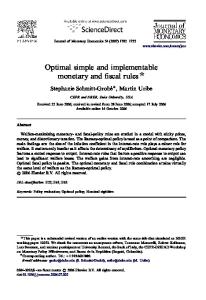
Since this equation characterizes monetary policy, we follow Taylor (1995) in referring to its graph as the MP curve. In (n, i)-space, the slope of the MP curve is positive. An increase in n lowers unemployment, leading to an interest rate hike. Lower unemployment also causes the real cost of labor to rise, leading firms to raise prices. The rise in capacity utilization also encourages firms to raise prices. The rise in inflation leads to an additional interest rate hike. 4

Goodfriend (1993) and Broadhaus (1995) have argued that this is even true when other instruments appear prominent: for example, when the funds rate has been targeted indirectly via manipulation of the discount rate or borrowed reserves. Cook (1989) goes even farther, arguing that even during the October 1979–October 1982 period most federal-funds-rate changes reflected judgmental actions of the Fed.

4

Algebraically the MP slope is ¯ di ¯¯ = iπ πn + iπ πω ωu un + iu un > 0 dn ¯MP As Goodfriend (1993,p.5) notes, use of an interest rate instrument effectively sets “money to the side, since at any point in time money demand is accommodated at the going interest rate.” However, as Post Keynesian structuralists have emphasized, this does not imply a horizontal MP curve, since the monetary authority responds to current economic conditions. The slope of the MP curve represents the responsiveness of monetary policy to inflation and unemployment. We see that the monetary authority’s policy parameters (iπ and iu ) determine the steepness of the MP curve. These parameters capture the marginal response of the monetary authority to economic conditions.

i

¡

MP

¡ ¡

¡

¡ ¡

¡ ¡

¡

¡

¡

¡

¡

¡

¡

¡

¡

n

Figure 1: MP Curve The reference levels π ¯ and u¯ are also important for the MP curve. A lower π ¯ or higher u¯ will shift up the MP curve. There is one other important shift factor for the MP curve: ns . Naturally a rise in ns implies a rise in u at any n, leading directly to a shift down in the MP curve. The indirect effect reinforces this downward shift: higher unemployment lowers the real cost of labor, allowing firms to moderate their price increases. These effects of changes in relative factor supplies will prove important for adjustment dynamics.

2

Equilibrium Unemployment

Unemployment rates at a point in time are determined in typical Keynesian fashion: output and employment adjust to a level compatible with goods market clearing. 5

2.1

Desired Investment

Firms desire to invest if the interest rate is right: κ(i − π). Here the function κ represents firms’ desired rate of growth of the capital stock, where i is the nominal interest rate, π is the rate of inflation. The behavioral response to an increase in the cost of borrowing is negative, κr < 0. The desired growth rate of capital stock is κ = κ(i − π) Recalling that π is determined according to (3), we can write ¡ ¢ κ = κ i − π[n, ω(u)]

(6)

(7)

Recall that the inflation rate π is increasing in n. At a given nominal interest rate, we find that (at any given i) an increase in the rate of capital utilization encourages firms to raise prices, and the aggregate result of increased inflation stimulates investment by reducing the real interest rate. This is reinforced through the effect on the unemployment rate: at a lower rate of unemployment, workers are able to push up the real cost of labor, and firms accelerate their price increase in response. Algebraically, we can characterize these arguments as follows: dκ = −κr (πn + πω ωu un ) > 0 dn

2.2

(8)

Desired Saving

National saving is determined by the private saving rate s and the government saving rate τ − g. S n = ((1 − τ )s + τ − g)Y (9) Given s, an increase in current income produce increases in private saving, but the change in government saving depends on the marginal propensity to deficit spend. This means that we cannot determine the response of saving to income, which depends on fiscal policy decisions.5 5

Some economists argue that the saving rate should be decreasing in labor’s share of income. We can characterize the wage share in terms of relative factor use n and the real cost of labor ω. The wage share is W N/P Y = ωAN/Y = ωn/y(n)

(10)

Since n/y(n) is increasing in n, we find that the wage share is increasing in n as well as in ω. Furthermore, we must recall that ω = ω(u) with ωu < 0. So W N/P Y = ω(u)n/y(n)

(11)

An increase in n reduces u and thus raises ω, which again decreases the saving rate by increasing labor’s share of income. We can therefore characterize national saving as S n /K = s(n, ns , τ ) + (τ − g)y(n)

6

(12)

We can turn (9) into an implied rate of change of the capital stock: S n /K = ((1 − τ )s + τ − g)Y /K

(13)

The output-capital ratio is determined in a standard fashion. Let aggregate output Y be determined by a first degree homogeneous production function: Y = F (AN, K)

(14)

Here K is the aggregate capital stock, N is the input of labor hours, and A indexes the level of technological progress in the following sense: technological progress A augments labor hours N to an effective labor input of AN . Output growth is determined by the growth of capital and effective labor inputs. The output-capital ratio is 1 y = F (AN, K) = F (AN/K, 1) = y(n) (15) K where n = AN/K can be characterized as the rate of capacity utilization. Note that y 0 > 0, capturing the stylized fact that capacity utilization is strongly procyclical.6 So our saving function becomes σ(τ, g, n) = ((1 − τ )s + τ − g)y(n)

(16)

where 1 > στ > 0, σg < 0, and σn = ((1 − τ )s + τ − g)y 0 . Note that the sign of σn matches the sign of ((1 − τ )s + τ − g).

2.3

IS Curve

Given out discussion of saving and investment behavior, equation (17) is a standard representation of goods market equilibrium. ¡ ¢ κ i − π[n, ω(u)] = σ(τ, g, n) (17) We will refer to the combinations of i and n such that (17) holds as the IS curve. For the reasons we have laid out, the slope of the IS curve is indeterminate. However we can pin down certain shifts in the IS curve. An increase in the tax rate will raise national saving, producing a shift down of the IS curve. An increase in the rate of government expenditure g will reduce national saving, producing a shift up of the IS curve. An increase in ns will increase unemployment at each n, producing a fall in the real cost of labor, a reduction in inflationary pressures, a rise in the real interest rate, and a fall in desired investment. This IS curve shifts down.7 where sns > 0 and sτ + y > 0.In this case, we are uncertain whether a rise in n augments or diminishes the private saving rate. Rose (1966) offers an extensive discussion of the determination of the warranted growth rate in his seminal paper on Keynesian growth models. He shows that setting s(n) offers a fairly general specification of saving behavior given competitive factor markets. For example, the saving specification of Kaldor (1966) can be transformed to this form in a Keynesian setting. 6 It also gives us procyclical productivity of the capital stock, in line with another stylized fact. Procyclical productivity of the labor is harder to capture. 7 If we were to add that an increase in ns increases saving by shifting the income distribution away from labor, this would also imply that the IS curve shifts down.

7

3

Temporary Equilibrium

This section characterizes equilibrium in our conflicting claims economy. We find that the monetary and fiscal policy parameters influence macroeconomic outcomes, influencing the distribution of income and the steady state unemployment rate. i

@

¡ ¡

@

@

@

¡

MP

i

¡

@¡ ¡@

¡

¡

¡ ¡

MP

i

¡ IS ¡ ©© © ¡© ©

¡ ©

@

¡

@

@ @ IS

¡

¡ ©© ©©¡ ¡ ¡

n

¡ ¡

IS

¡ MP ¡ ©© © ¡© ¡© © ¡ ©© ©©¡ ¡ ¡

n

n

Figure 2: Temporary Equilibrium

3.1

Model Summary

For convenience of reference, table 1 summarizes the model of temporary equilibrium. (2)

Wage Adjustment

(3)

Price Adjustment

(4)

Monetary Policy

(15)

Output and Capacity

(17)

Goods Market Equilibrium

ω = ω(u) ω0 < 0 π = π(n, ω) πn , πω > 0 i = i(π − π ¯ , u − u¯) iπ > 0, iu < 0 y = y(n) y0 > 0 κ(i − π) = σ(τ, g, n) κr < 0

Table 1: Inflation and Unemployment with Endogenous Money As an even briefer summary, this model can be partially reduced as follows: MP Curve IS Curve

i = i(π[n, ω(u)] − π ¯ , u − u¯) κ(i − π[n, ω(u)]) = σ(τ, g, n)

Figure 2 graphs (17) and (5) in i, n-space (for a given level of ns ). The IS curve is basically familiar (although it builds in some new considerations), and our Taylor-rule characterization of monetary policy replaces the traditional LM curve. When the natural growth rate 8

and warranted growth rate differ, the economy does not rest at the temporary equilibrium represented by the intersections in figure 2. To see why, reconsider the growth dynamics embodied in (21). If the natural rate of growth exceeds the warranted rate of growth, so that capital formation does not keep up with the growth of effective labor, then ns rises.

4

Natural vs. Warranted Growth

The natural growth rate is determined by the growth rates of the labor force and technological change. Let N s be the available supply of labor hours. Technological progress augments this to an effective labor supply of AN s , where A indexes the level of technological progress. The natural rate of growth gAN is just the growth rate of the effective labor supply: b+N cs [s = A gAN = AN

(18)

where a b indicates a percentage rate of change. Unless the natural rate of growth is warranted by aggregate saving, the economy will experience labor market dislocations. To see this, define the relative factor supply ns by ns = AN s /K

(19)

Then we can characterize the growth rate of ns by n ˆ s = gAN − gK

(20)

where gK is the actual rate of capital accumulation, as determined by aggregate saving and investment behaviors. So ns rises or falls as the natural rate of growth (gAN ) is greater than or less than the warranted rate of growth (gK ). In a steady state, the warranted rate of growth equals the natural rate of growth, and gK = gAN . Models in the tradition of Keynes differ from those in the neoclassical tradition by specifically allowing that aggregate demand deficiencies can produce persistent involuntary unemployment. An economy experiences unemployment when the available supply of labor hours is greater than the amount of labor hired: N s > N , where N is the actual input of labor hours into the production process. In terms of effective-labor to capital ratio, we rewrite this as ns > n, where we recall that we may interpret n = AN/K as the labor intensity of production or as the rate of capacity utilization. Most business cycle variation in hours worked is due to changes in number of workers employed rather than in hours per worker (Goodfriend and King 1997). While the present paper does not explicitly distinguish these two sources of variation, short-run movements in N are best conceived as movements in the number of workers employed. The evolution of the potential labor intensity of production is therefore determined as follows: n ˆ s = gAN − σ(τ, g, n) (21) Equation (21) implies that the evolution of the unemployment rate is affected by economic growth. At any given n, unemployment rises or falls as the natural rate exceeds or fall short of the warranted rate of growth. This is the source of the model’s adjustment dynamics. 9

4.1

Model Summary

For convenience of reference, we can summarize the model as follows. MP Curve IS Curve Growth Dynamics

4.2

i = i(π[n, ω(u)] − π ¯ , u − u¯) κ(i − π[n, ω(u)]) = σ(τ, g, n) n ˆ s = gAN − σ(τ, g, n)

Adjustment Dynamics

One of the experiments we considered during the development of the IS and MP curves was the effect of a change in ns . We found that an increase in ns would shift down both the IS and the MP curves. An increase in ns means greater unemployment at each value of n, which leads the monetary authority to lower interest rates. Higher unemployment produces a fall in the real cost of labor, which reduces the pressure on firms to raise their prices. The resulting lower inflation rates again lead the monetary authority to lower interest rates. In the IS-MP diagrams of figure 3, this is represented by a downward shift in the MP curve to MP0 . However the IS curve is also affected by the lower inflation rates: the IS curve also shifts down. The effect on n depends on the relative size of these two shifts and on the relative slopes of the IS and LM curves. The evolution of the macroeconomy depends on sizes of these shifts and on the slopes of the curves. i

@

@

@

¡

@

@

¡

@

¡

¡

¡

¡ ¡

MP

i

MP0

¡ @¡ ¡ @ @¡ @ ¡ @ ¡ @ ¡ @ ¡ @ ¡ @ ¡ ¡ @ @ ¡ ¡ @ @ IS ¡ ¡ @ @ IS0 @

n ¯

MP

@ ¡ @@ ¡ MP0 @@ ¡ ¡ @@ ¡ ¡ @@ ¡ ¡ @@ ¡ ¡ @ ¡@ ¡ ¡ @ ¡@ ¡ ¡ @@ @@ ¡ ¡ @@ ¡ ¡ @@ ¡ ¡ IS @ IS 0

n

n ¯

n

Figure 3: Adjustment Dynamics The key question for macroeconomic stability of the adjustment dynamics is whether increases in ns increase the warranted rate of growth. More formally, (21) implies that a steady state will be stable if dˆ ns 0, κns = −κr πω ωu uns < 0, in = iπ (πn + πω ωu un ) + iu un > 0, and ins = (iπ πω ωu + iu )uns < 0. Then we can write this system more compactly as κr di + κn dn − σn dn = −κns dns di − in dn = ins dns Solving for the reduced form responses we get · ¸· ¸ · ¸ kr (kn − σn ) di −κns dns = 1 −in dn ins dns · ¸· ¸ ¸ · 1 −in σn − kn −κns dns di = kr ins dns dn σn − kn − kr in −1

(28) (29)

(30)

We are particularly interested in the implied sign of nns . This however is indeterminate: 1

[κns + kr ins ] σn − kn − in kr 1 [κns /kr + ins ] = (σn − kn )/kr − in

nns =

(31)

Intuitively, in order to determine the sign of nns , we need to know two things: the relative slopes of the IS and LM curves, and the relative speeds with which they shift down in response to an increase in ns . Note that the slope of the IS curve is −(κn − σn )/κr and the slope of the MP curve is in . So the relative slopes of the two curves matter. In the traditional case, the MP curve has the greater slope. Now what about the term κns /kr + ins ? Noting that κns /kr + ins = −πω ωu uns + (iπ πω ωu + iu )uns = [(iπ − 1)πω ωu + iu ]uns 8

Recall σn = ((1 − τ )s + τ − g c − g i )y 0 is indeterminate in sign because of the possible dissaving by government.

11

we find we can sign this unambiguous (as negative) when the monetary authority responds aggressively to inflation. This is just a sufficient condition for the MP curve to shift down faster than the IS curve in response to an increase in ns . The IS curve shifts down at rate -κns /kr . The MP curve shifts down at rate ins . This highlights the importance of monetary policy for economic stability. The responses of monetary policy to inflation and unemployment affect macroeconomic stability. In these broad terms, the observation is not new. For example, it is often proposed that a simple interest rate peg destabilizes the economy. We now explore this possibility.

5

Interest Peg

Is it destabilizing for the monetary authority to set an arbitrary interest peg? The traditional suspicion is that this destabilizes the economy unless the monetary authority has the incredible wisdom or luck to peg at just the right level. However we find the situation to be more complex. i

i

@

@ @ @ @ @ @ @ @ @ MP @ @ @ @ @ @ @ @ @ @ @ IS0@ IS n ¯

IS

¡ ¡ IS0 ¡ ¡ ¡ ¡ ¡ ¡ ¡ ¡ MP ¡ ¡ ¡ ¡ ¡ ¡ ¡ ¡ ¡ ¡ ¡ ¡

n

n ¯

n

Figure 4: Adjustment Dynamics: Interest Peg Recall that stability requires −σn [κns /kr + ins ] < 0 (σn − kn )/kr − in No interest rate responses turns this into −σn κns /kr < 0 (σn − kn )/kr −σn κns < 0 (σn − kn ) Since we know kn > 0 and kns < 0, we already know σn > 0 is required for stability. That is, intuitively enough, it is important for deficit spending not to soak up all the available private saving. 12

However stability also requires that the government not run huge surpluses (at the margin). This is just the requirement that the IS curve have a positive slope (in this case). σn 0. In order to explore the long-run effects of such a change, we consider the long-run comparative statics of the model. That is, we determine n, ns , and i under the constraint that n ˆ s = 0. Our model summary becomes: MP Curve IS Curve Growth Dynamics

i = i(π[n, ω(u)] − π ¯ , u − u¯) κ(i − π[n, ω(u)]) = σ(τ, g, n) 0 = γ − σ(τ, g, n)

Long-run capacity utilization, n ¯ , is the level that equates the natural and warranted growth rates. This long-run relationship is represented by 0 = γ − σ(τ, g, n ¯ ). Given this long-run level of capacity utilization, we can determine the effects on i and ns . κr di + κns dns = 0 di − ins dns = −iπ d¯ π · ·

di dns

kr kns 1 −ins

¸ =

k ns

¸·

−1 + kr ins

¸ · ¸ di 0 = dns −iπ d¯ π ¸· ¸ · 0 −ins −kns −1 kr −iπ d¯ π 13

(34) (35)

(36) (37)

i

i

¡

@ @

@

@

@

MP

@

¡ ¡ ¡ M P SR @ ¡ ¡ ¡ @ ¡ ¡ @¡ ¡ ¡ @¡ ¡ ¡@ @ ¡ ¡ @ @ IS ¡ ¡

M P LR

¡ ¡

@ ¡ @¡ ¡@ @ ¡ @ ¡

@

¡ ¡

¡

@

@ @ IS LR

¡

n

n

Figure 5: Short-Run and Long-Run Effects of an Increase in π ¯

dns kr iπ = d¯ π kns + kr ins iπ = kns /kr + ins

(38)

Recalling κns = −κr πω ωu uns < 0 and ins = (iπ πω ωu + iu )uns < 0, we might despair of signing this. But let us continue: iπ dns = d¯ π −πω ωu uns + (iπ πω ωu + iu )uns iπ = [(iπ − 1)πω ωu + iu ]uns

(39)

So we find that as long as the monetary authority reacts adequately to inflation, we can sign this: dns