Modelling Hydrokinetic Energy Resource for In-stream Energy Converters
Emilia Lalander
UURIE 316-10L ISSN 0349-8352 Division of Electricity Department of Engineering Sciences Uppsala, January 2010
Abstract
Hydrokinetic energy, referring to the energy contained in moving water, is a renewable energy source that has gained much attention the past years. The energy is found in all moving water masses, but is only economical to convert for water masses moving with high velocity, i.e. likely around 1 m/s and above. This energy can for example be found in tidal, ocean and river currents which flow through narrow straits and channels. Along the west coast of Norway, there are many sites where kinetic energy conversion would be possible due to the strong current present. The driving force behind the currents is the tidal wave that progresses northward along the coast and increases in strength. The models that so far have been used for estimating the resource in Norway, have been shown to be uncertain since they do not account for the fact that the velocities and the water levels are altered when energy is extracted. These effects can be simulated with numerical models. A channel in the Dal river, the Söderfors channel, is situated downstream a hydropower plant and was simulated with the numerical model MIKE. The water level alteration due to turbines was simulated. It was shown to be a lot less than the water level alteration caused by the level change in the downstream lake. Velocity profiles measured at several different locations were used to estimate how the power coefficient was changed. Four turbine configurations were studied and it was shown that changes in the power coefficient were prominent only for a vertical shear profile with a strong gradient. At the Division of Electricity, studies have been conducted on how to convert hydrokinetic energy to electricity since 2003. The main idea has been to use a system that limits the need for maintenance. The concept studied is a vertical axis turbine directly coupled to a permanent magnet generator. The Söderfors channel has, due to aspects such as the flow properties and velocity, been chosen as a site for an experimental station.
To my family
List of Papers
This thesis is based on the following papers, which are referred to in the text by their Roman numerals. I
II
III
IV
V
Grabbe, M., Lalander, E., Lundin, S. (2009) A review of the tidal current energy resource in Norway Renewable and sustainable energy reviews, 13(8):1899–1909 Lalander, E., Leijon, M. (2009) Numerical modelling of a river site for in-stream energy converters Proceedings of the 8th European Wave and Tidal energy conference, Uppsala, Sweden, 2009 Lalander, E., Leijon, M. In-stream energy converters in a river – effects on upstream hydropower station Submitted to Renewable energy, September 2009 Goude, A., Lalander, E., Leijon, M. (2009) Influence of a varying vertical velocity profile on turbine efficiency for a vertical axis marine current turbine Proceedings of the ASME 2009 28th International Conference on Ocean, Offshore and Arctic Engineering Grabbe, M., Yuen, K., Goude, A., Lalander, E., Leijon, M. (2009) Design of an experimental setup for hydro-kinetic energy conversion Hydropower and Dams, 15(5): 112–116
Reprints were made with permission from the publishers.
Nomenclature
Notation A At B c CD Cf Cp CS d f Ft g h hf ht L λ n N ρ P p Pw Q ω R Rh σ τ V
= = = = = = = = = = = = = = = = = = = = = = = = = = = = = =
Cross-section area of the channel [m2 ] Cross-section area of the turbine [m2 ] Width of channel [m] Chord length [m] Turbine drag coefficient Friction coefficient Power coefficient Smagorinsky coefficient Bottom elevation from the datum line [m] Darcy-Weisbach friction factor Force of turbine on the water [N] Acceleration due to gravity [m/s2 ] Channel depth [m] Head loss caused by friction [m] Head loss caused by turbines [m] Channel length [m] Tip speed ratio Manning number [s/m1/3 ] Number of turbine blades Density [kg/m3 ] Power [W] Pressure [N/m2 ] Wetted perimeter [m] Discharge [m3 /s] Angular velocity [rad/s] Turbine radius [m] Hydraulic radius [m] Solidity Shear stress [N/m2 ] Current speed [m/s]
Subscripts f t 0 1 2 3 4
= = = = = = =
related to bottom friction related to the turbine undisturbed section before turbine at the turbine immediately after the turbine in the wake after the turbine outside the wake
Abbreviations ADCP = DMS = DNL = MMSS =
Acoustic Doppler Current Profiler Double Multiple Streamtube Den Norske Los Mean maximum spring speed
Contents
1
2
3
4
5
6
7
8
Introduction . . . . . . . . . . . . . . . . . . . . . . . . . . . . . . . . . . . . . . . . . . 1.1 Thesis layout . . . . . . . . . . . . . . . . . . . . . . . . . . . . . . . . . . . . . . 1.2 Hydrokinetic energy conversion . . . . . . . . . . . . . . . . . . . . . . . . 1.2.1 Tidal energy devices . . . . . . . . . . . . . . . . . . . . . . . . . . . . 1.3 Energy extraction in rivers in Sweden . . . . . . . . . . . . . . . . . . . 1.4 The project at Uppsala University . . . . . . . . . . . . . . . . . . . . . . Resource assessments . . . . . . . . . . . . . . . . . . . . . . . . . . . . . . . . . . . 2.1 Methodology for calculating the resource . . . . . . . . . . . . . . . . . 2.2 Resource in Norway . . . . . . . . . . . . . . . . . . . . . . . . . . . . . . . . 2.3 Other models used for resource estimates . . . . . . . . . . . . . . . . . Channel and turbine theory . . . . . . . . . . . . . . . . . . . . . . . . . . . . . . . 3.1 Influence of bottom friction on channel flows . . . . . . . . . . . . . . 3.2 Influence of turbines on channel flows . . . . . . . . . . . . . . . . . . . 3.3 Turbines in a constricted channel . . . . . . . . . . . . . . . . . . . . . . . 3.4 Properties of the turbine power coefficient . . . . . . . . . . . . . . . . Current measurements . . . . . . . . . . . . . . . . . . . . . . . . . . . . . . . . . . 4.1 About the ADCP . . . . . . . . . . . . . . . . . . . . . . . . . . . . . . . . . . . 4.2 Field work . . . . . . . . . . . . . . . . . . . . . . . . . . . . . . . . . . . . . . . . Models and methods . . . . . . . . . . . . . . . . . . . . . . . . . . . . . . . . . . . 5.1 Channel model . . . . . . . . . . . . . . . . . . . . . . . . . . . . . . . . . . . . 5.1.1 Simulation setup . . . . . . . . . . . . . . . . . . . . . . . . . . . . . . . 5.1.2 Validation of the model . . . . . . . . . . . . . . . . . . . . . . . . . . 5.1.3 Including turbines . . . . . . . . . . . . . . . . . . . . . . . . . . . . . . 5.2 Turbine model . . . . . . . . . . . . . . . . . . . . . . . . . . . . . . . . . . . . . 5.2.1 Method . . . . . . . . . . . . . . . . . . . . . . . . . . . . . . . . . . . . . . Results and discussion of channel and turbine models . . . . . . . . . . . 6.1 Influence of turbines in a channel . . . . . . . . . . . . . . . . . . . . . . . 6.2 Effects on CP of different turbine configurations, shear profiles and solidity . . . . . . . . . . . . . . . . . . . . . . . . . . . . . . . . . . . . . . . The site in Söderfors . . . . . . . . . . . . . . . . . . . . . . . . . . . . . . . . . . . 7.1 Site characterization . . . . . . . . . . . . . . . . . . . . . . . . . . . . . . . . 7.2 Experimental set-up . . . . . . . . . . . . . . . . . . . . . . . . . . . . . . . . . 7.3 Annual energy output . . . . . . . . . . . . . . . . . . . . . . . . . . . . . . . 7.3.1 Velocity distribution . . . . . . . . . . . . . . . . . . . . . . . . . . . . . 7.3.2 Turbine and generator . . . . . . . . . . . . . . . . . . . . . . . . . . . Conclusions . . . . . . . . . . . . . . . . . . . . . . . . . . . . . . . . . . . . . . . . . .
11 11 11 12 12 13 15 15 16 17 19 19 20 20 22 25 25 26 29 29 30 30 31 31 32 35 35 36 39 39 40 40 40 42 45
9 10 11 12 13
Future studies . . . . . . . . . . . . . . . . . . . . . . . . . . . . . . . . . . . . . . . . Summary of papers . . . . . . . . . . . . . . . . . . . . . . . . . . . . . . . . . . . . Sammanfattning . . . . . . . . . . . . . . . . . . . . . . . . . . . . . . . . . . . . . . . Acknowledgements . . . . . . . . . . . . . . . . . . . . . . . . . . . . . . . . . . . . References . . . . . . . . . . . . . . . . . . . . . . . . . . . . . . . . . . . . . . . . . . .
47 49 51 53 55
1. Introduction
1.1
Thesis layout
This licentiate thesis is part of the marine current group at the Division of Electricity at Uppsala University. The aim of the project is to study a concept for converting kinetic energy of water to electricity, and this thesis is concerned with finding a site for the energy extraction. The main contribution of the author has been to measure current velocities at various locations in Sweden, and combine these with numerical models of channels and turbines. In Ch. 2 a description of the tidal current energy resource in Norway is made with the aim of introducing the reader to how previous resource assessments have been done. In Ch. 3 some channel flow theories and descriptions of numerical models for channel flows are presented. This is followed by a description of the current measurements that have been made in Ch. 4. The results of the modelling and current measurements are presented and discussed in Ch. 5. The last chapter (Ch. 7) is about defining the site for the experimental station in Söderfors.
1.2
Hydrokinetic energy conversion
The increased demand for electric energy has spawned new technologies for extracting energy from the ocean. This is however not an easy task due to the harsh environment in the ocean. Several of these technologies have been faced with difficulties, sometimes to a complete breakdown, and as of today there are only a handful of concepts in the world that successfully produce electricity for the grid. Still, the research is progressing fast and the industry will continue to grow as the attention has increased for these types of renewables. One renewable energy source found in the ocean is tidal energy, whose main source is the gravitational pull between the earth and the moon creating a tidal wave that progress across the oceans. Due to resonance effects, ocean depth etc. the wave will appear differently in the different parts of the world. At the west coast of Sweden, the height of the tidal wave is approximately 0.5 m1 , whereas in the Bay of Fundy (Canada) the tidal wave can exceed 15 m in height [1]. The tidal wave will give rise to strong currents in narrow sections, sometimes reaching more than 4 m/s. Many of the sites with strong 1 SMHI:
http://www.smhi.se/vadret/hav-och-kust/havsobservationer/havsvst.htm
11
tidal currents are known by sailors and seamen as they are dangerous to pass. These areas are thus seldom well studied and are often quite remote, which is one of the reasons this industry is still in its preliminary stages. Despite the fact that there are many sources to the kinetic movement of water, the main part of the industry regarding hydrokinetic energy extraction is focused on sites with strong tidal currents. Common names for the energy capturing devices are thus Tidal In-Stream Energy Converters (TISEC [2]) or Marine Current Turbines, i.e. names that connect the devices to the ocean. Here we propose to use the term hydrokinetic energy converters, which can include both ocean and river currents.
1.2.1
Tidal energy devices
The two largest devices that are in operation today are the Open Hydro2 (1 MW) and MCT (Marine Current Turbines Ltd3 ) (1.2 MW) devices. There are, however, many other projects being built and tested, many of which can be found at the webpage of EMEC4 (The European Marine Energy Centre).
(a) Open Hydro
(b) MCT
(c) HS1000
Figure 1.1: The two largest turbines operating today: Open Hydro (a) and Marine Current Turbines (MCT) (b). The 1 MW turbine from Hammerfest Strøm (c) will be installed in 2010.
Similar concepts as the ones used in the tidal industry can be applied in rivers, but then usually in smaller scale. As these concepts are likely to have small impact on the environment, they can in the future provide a significant contribution to electricity production in rivers protected from e.g. regulation. Today there are various small scale prototypes being tested in rivers, of which many can be read about in [3].
1.3
Energy extraction in rivers in Sweden
As the tidal height is low around the coast of Sweden and only present on a daily basis in the west coast of Sweden, the tidal velocities are low. For the purpose of energy extraction, it has thus been more reasonable to explore the 2 http://www.openhydro.com 3 http://www.marineturbines.com 4 http://www.emec.org.uk/tidal_developers.asp
12
potential in rivers. Since the kinetic energy flux is proportional to the cube of the velocity, rivers with a high mean flow are more likely to be suitable for implementation of concepts such as the ones shown in Fig. 1.1. 2500 Unregulated river Regulated river
flow / m3/s
2000 1500 1000 500 0 1998
1999
2000
2001
2002
Figure 1.2: Example of flow situation in a regulated river (Lule river) and an unregulated river (Kalix river), both situated in the north of Sweden. Data from SMHI
In Sweden there are approximately 8 rivers with a mean flow above 300 m3 /s 5 , of which most are located in the north. All but four rivers are to a larger or lesser extent regulated by hydropower. On a year with normal flow, the electricity production in Lule river (Fig. 1.2) corresponds to 21% of the total electricity production for hydropower in Sweden [4]. During the year 2000 the four largest regulated rivers in the north produced 2/3 of the total hydropower production in Sweden. The driving mechanism of river flows is the potential energy the water gains as it precipitates on land and accumulates in river channels. River flows are not as predictable as tidal flow. The yearly flow variation in two of the larger rivers in Sweden is shown in Fig. 1.2. One river is regulated and the other is unregulated, the former having daily flow variations while the variations in the latter are seasonal.
1.4
The project at Uppsala University
At the Division of Electricity, a project is on-going about constructing a device that converts kinetic energy of river flows to electricity. The standpoint is to have a vision of the entire system, from water currents to grid connexion. Every step has to be built to minimize the need for maintenance. This is done by building a robust system with few moving parts. The proposed turbine is an omni-directional vertical axis turbine, thus not needing any yaw mechanism, connected directly to the generator. It can be deployed in channels or river courses without requiring any dams. The system is designed to be able to convert the slow movements of the water to electricity. In 2007 the first generator was built [5, 6]. As of 2009 a site has been found in Dalälven, the Dal river, downstream of the hydropower 5 Vattenportalen:
http://www.vattenportalen.se/fov_sve_djup_sot_vattendrag.htm
13
station in Söderfors. Here the first experimental station is planned to be built, and this is discussed in further depth in Ch. 7.
14
2. Resource assessments
The purpose of this chapter is to give an insight into the resource estimates that have been made for tidal energy in Europe, with a special focus on Norway. This chapter contains a brief summary of Paper I which is a review paper regarding the tidal energy potential in Norway. The review article was conducted to emphasize the uncertainty of the result of the tidal resource estimates in Norway.
2.1
Methodology for calculating the resource
Hydrokinetic energy conversion has gained much attention the last decade and several reports now exist on the extractable potential (see end of this section) for marine current energy. In 1996 a report to the European Commission [7] suggested the yearly potential for tidal energy in Europe was 48 TWh, of which most could be found around the UK. The methodology was revised in [8] and [9] for the UK resource and although it was pointed out that there was a considerable uncertainty of the result, the conclusions were that 18 TWh could be extracted around the UK each year. These reports are based on questionable data, but still point toward a great potential for this type of renewable energy source. A review on the subject can be found in [10]. Many resource estimates, e.g. in [9, 11, 12], are commenced by calculating the power in a free flow. The power in a water mass with density ρ and a velocity V through a cross-sectional area A is 1 P = ρAV (z)3 . 2
(2.1)
The velocity is assumed to vary with depth according to a power law V (z) = V0
� h(z) �1/α h
,
(2.2)
where α is usually 6, 7 or 10, a number that depends on the roughness of the sea bed, V is the velocity and h is depth. Assuming the flow has shear with α = 10, the mean power in the flow will be proportional to V 3 = 0.769V 3 .
(2.3)
15
The velocity of a tidal current is then assumed to vary linearly with the amplitude of the tidal wave (see Fig. 2.1), i.e. sinusoidally. The maximum velocity is the mean maximum spring speed (MMSS). Further on, the velocity is assumed lower at neap tide than at spring tide, lower for the second tide than the first and lower for the flood tide than for the ebb tide. Thus integrating Eq. 2.1 for an entire year, the total energy output is achieved.
m
2
Flood
0 −2
Ebb 2
4
6
1st and 2nd tide Spring and neap tide 8 10 12 14 16
18
20
Figure 2.1: Tidal height variation in October 2009, Great Hill, US. Data from http://tidesandcurrents.noaa.gov/
Tidal current potential has been referred to as theoretical, extractable, technical and economical potential, all carrying different assumptions, for which other constants are multiplied into Eq. 2.1. The theoretical resource is defined as the raw flux of energy through a cross section of a site and is proportional to the cube of the velocity according to Eq. 2.1. For information on how to calculate the extractable, technical and economical potential see e.g. [8, 12]. For more details on the assumptions, see [12].
2.2
Resource in Norway
Along the Norwegian coast there is undoubtedly a large potential for tidal power. The tidal wave that departs the northern tip of Great Britain increases in amplitude along the Norwegian coast due to the shallow continental shelf (Fig. 2.2). The narrow constrictions in the many fjord outlets cause a phase shift in the tidal amplitude in- and outside the fjord which causes strong velocities. There have been three reports on the resource estimates for Norway; One report was a master thesis [11], one was made by private consultants [13] and the last being the review in Paper I. All reports have used the method described in Sec. 2.1. The last report was conducted to emphasize the uncertainty that follows with using this method. In Paper I the theoretical resource was calculated for the entire coastline of Norway, using the same method as in [11]. Velocity data was taken from Den Norske Los (DNL) with the assumption that the MMSS varied linearly with the tidal amplitude. The difference between the first and second tide was 16
HWL 4
200 100
phas e
delay
2 Reference water level
0 −100
lo Os
−2
LAT
−200
−4
LWL
rg Be
en n Tro
dh
ei m
0
time / hours
water level / cm
HAT
d Bo
ø
t ø ms rfes Tro mme a H
rdø Va
Figure 2.2: Sea level along the Norwegian coast shown as highest and lowest water level (HWL/LWL) and highest and lowest astronomical tide (LAT/HAT) compared with the mean water level.
set to 93.6% while the difference between spring and neap was set to 79.6%. Although the same method was used as in [11], the assumptions were different and thus many more sites were considered in Paper I. While only velocities above 2 m/s and depths larger than 6 m were considered in [11], all velocities above 1 m/s were considered in Paper I, resulting in 104 sites instead of only 12. In [13] 22 sites were considered, with the criteria that the MMSS should be higher than 1.5 m/s, the operational time 3500 h/year, a 50% coverage of the cross-sectional area and a 40% total system efficiency. Model sensitivity The results are presented in Table 2.1. It is clear that the variation among the different models is large, although they are based on the same data. The two variables used in Eq. 2.1 are the velocity and the cross-sectional area. Since the power depends on the velocity cubed, any uncertainties in the velocity will result in that the error is cubed and it is therefore important that the value of the velocity is accurate. The result presented in Table 2.1 shows the large variability, and thus the uncertainty, of using this method and on using the DNL as a source for data for estimating the resource. The information in the DNL has been written down mainly for navigational purposes, and have not been intended to be used as basis for resource estimations.
2.3
Other models used for resource estimates
Due to the uncertainty connected with the above mentioned model, resource estimates have been calculated with the use of numerical models [14, 15, 16], 17
Table 2.1: A comparison of how the resource is distributed among different velocity and mean depth intervals in the three resource assessments. The number of sites is given for each interval followed by the contribution to the total resource as a percentage. From Paper I
No. of sites Theoretical resource Extractable resource Technical resource Economical resource No of sites with MMSS above 3 m/s MMSS of 2–3 m/s MMSS below 2 m/s mean depth of more than 40 m mean depth of 20– 40 m mean depth of less than 20 m
Fröberg [11] 12 2.3 TWh 0.23–1.1 TWh 0.18–0.89 TWh 0.16–0.82 TWh
Enova SF [13] 22 – – > 1 TWh < 1 TWh
Present study 104 17 TWh – – –
3 (41%) 9 (59%) – 1 (24%)
4 (6%) 11 (79%) 9 (15%) 11 (85%)
28 (68%) 39 (26%) 37 (6%) 15 (59%)
5 (52%)
11 (13%)
17 (28%)
6 (24%)
2 (2%)
72 (13%)
with analytical estimates of the resource in a channel linking a bay to the ocean [17, 18], or a combination of both [19]. These models calculate the potential for specific sites, and have not been used to calculate a total estimated European potential. However, the accuracy can be significantly improved since the models can be validated against current measurements [20], and a change in flow magnitude and surface levels can be taken into account. This will be further discussed in Chapter 6.
18
3. Channel and turbine theory
In this chapter the theories for channel flow and numerical models of the turbines that have been used for this work are described. The purpose is to give a brief introduction to the main causes of water level alteration in a natural channel (Sec. 3.1), how turbines alter the water level (Sec. 3.2), and how a constricted channel can increase the power output (Sec. 3.3)
3.1
Influence of bottom friction on channel flows
For a long channel with steady flow, the weight force component in the xdirection is balanced by the frictional forces at equilibrium. Since a long channel is considered, there will be a head loss in the flow direction caused by friction against the sea bed. The friction-induced head loss can be written hf =
τf L, ρgRh
(3.1)
where h f is the head loss, τ f is the shear stress, L is the channel length and Rh is the hydraulic radius equal to the cross sectional area divided by the wetted perimeter, Pw (Pw = B+2h where B and h are the width and depth respectively) [21]. hf H V
h τf
d
L Figure 3.1: Schematic view of a river with a steady, uniform flow with sloping bottom. h f is the head loss along the channel caused by friction τ f , H is the mean total energy, h the channel depth and d is the height above a reference line.
The shear stress, τ f is proportional to the cube of the velocity, V , and can be written in terms of the Darcy-Weisbach coefficient, f , or the Manning number, n, according to 19
f ρV 2 (Darcy) 8 ρgn2 = 1/3 V 2 (Manning), Rh
τf =
3.2
(3.2)
Influence of turbines on channel flows
A turbine placed in a channel with water that flows with a certain velocity will induce a force acting against the flow. The turbine force can be written in terms of a drag coefficient 1 Ft = CD ρAt V12 , 2
(3.3)
where V1 is the velocity through the turbine, At the turbine area and CD the drag coefficient. The turbine power is then simply Pt = Ft V1 . The turbine force against the flow induces a pressure force of equal strength written 1 P = ρgQ∆h, 2
(3.4)
where Q is the discharge and ∆h is the depth change. Thus, a turbine put in a channel will alter the water depth. The depth change caused by turbine energy extraction can be defined ht , simply written as ht =
P . ρgQ
(3.5)
The change in water level caused by turbines can be added to the left hand side of Eq. 3.1, i.e. to h f , to correspond to the total water level alteration in the channel.
3.3
Turbines in a constricted channel
In an infinitely wide channel, a turbine can be modelled as a disc through which some flow is allowed to pass. The pressure and velocity distribution for this situation is shown in Fig. 3.2(a). The force exerted by the turbine on the water, Ft , can be expressed either by a drag coefficient as in Eq. 3.3, or by the use of the pressure difference across the turbine:
20
1 Ft = (p1 − p2 )V1 . 2
(3.6)
To solve for the pressure difference across the turbine it is possible to use the Bernoulli equation: p V2 + dg + = constant, ρ 2
(3.7)
where p is the sum of atmospheric and hydrostatic pressure and d is the seabed elevation from a reference line (Fig. 3.1). The equation is valid for a steady incompressible flow, and is constant along a streamline [22, 21]. Applying the Bernoulli equation from the undisturbed area to the turbine (p0 to p1 ) and from the turbine to the wake (p2 to p0 ), the pressure difference over a turbine with cross-sectional area At can be written 1 p1 − p2 = ρAt (V02 −V32 ). 2
(3.8)
V0 V0 p0
V1 p1 p2 V 3
V4
V0 p0
V0
L
V1 p1 p2
p0
V3 p4 p4
(a) Unconstricted
V5 p5
(b) Constricted
Figure 3.2: Two channel views (a) No channel sides. The flow is allowed to expand to the sides (b) With channel sides. The flow is constricted.
In the case of the channel shown in Fig. 3.2(b), the constricting walls have to be taken into account. The velocity at the sides of the turbines, V4 , is then assumed to be higher than the free-flow velocity, V0 , but to avoid transverse velocities, the pressure outside and inside the wake is assumed to be equal [23]. Applying three Bernoulli equations from the undisturbed area to the turbine (p0 to p1 ), from the turbine to the wake section (p2 to p0 ) and from the undisturbed area to outside the wake (p0 to p4 ) the pressure difference across the turbine is obtained: 1 p1 − p2 = ρAt (V42 −V32 ). 2
(3.9)
Since the turbine power, Pt , is equal to the force of the turbine multiplied with the velocity, using Eq. 3.6 and 3.9 , the turbine power can be written 21
1 Pt = ρAt (V42 −V32 )V1 2
(3.10)
For a turbine in a free flow the maximum Pt is 59% of the incoming power (Fig. 3.2a). The incoming power, P, is defined by Eq. 2.1. For turbines in a constricted channel, it is theoretically possible to exceed this limit. This is illustrated in Fig. 3.3 where Pt /P is plotted against V3 /V0 (V3 is the wake velocity) and against CD . For a turbine that is small compared with the cross sectional area of the channel, Pt /P will approach 59%.
2.5
2.5
50%
2
50%
2
40%
1
40% 1.5
33.33% 26.67% 20%
Pt / P
Pt / P
1.5
33.33% 26.67%
1
20% 0.5 0 0
0.5
0.5 V3 / V0
1
0 0
10
20
30
40
50
CD
Figure 3.3: Maximum energy extraction possible depending on how large fraction of the cross-sectional area that is covered by the turbine, indicated by percentage values. From Paper III
There are of course several limitations to the model since e.g. no wall or bottom friction has been included, which would reduce the velocity at the sides of the turbine, V4 . Although it is interesting to note that a turbine in a channel with constricting walls could extract more power than it would if put in a free flow, for any real channel the maximum power capture would still be proportional to what is actually available. In a river site, this would be the total head of the river. The model does not account for any limitation in the head drop before and after the turbine. The interested reader is recommended to see references [23, 17, 24].
3.4
Properties of the turbine power coefficient
The turbine is essentially the energy-capturing device. There are several different turbine concepts where most can be divided into cross-stream and streamaligned turbines. Here we focus on a cross-stream turbine. The cross-stream turbine studied here has the advantage of not needing a yawing mechanism since it is independent of the flow direction. It is also possible to change the ratio of the width and height of the turbine, so that the turbine can be uniquely designed to suit a channel. 22
The turbine power coefficient is defined as the quotient of the turbine absorbed power divided by the power in the undisturbed flow CP =
Pt 0.5ρAt V 3
(3.11)
The tip speed ratio, λ , is the quotient of the speed of the turbine at the blade tip (same for the whole blade for the turbine in the focus of our study) divided by the velocity in the undisturbed flow: λ=
Rω . V (z)
(3.12)
For a constant radius and height, the turbine performance, commonly described with a CP vs. λ -curve, will depend mainly on the solidity, which is defined as σ=
Nc , 2πR
(3.13)
where N is the number of turbine blades, c is the blade chord length and R is the turbine radius.
Figure 3.4: A c p – λ curve.
23
4. Current measurements
In this chapter a basic description of the current measurements that have been made is presented. Measurements were conducted to identify sites with high current velocities and to study the velocity profile at each site.
4.1
About the ADCP
In order to measure currents, Acoustic Doppler Current Profilers (ADCP, Fig. 4.1) from RD Instruments have been used. The instrument is a common tool utilized in oceanographic research. For different instrument accuracy and sensor size it is capable of measuring from a few meters water depth to several hundreds of meters with a time frequency down to 1 Hz.
Figure 4.1: A 1200 kHz ADCP
The instrument uses broadband technology where current velocities are determined by emitting sound with a certain frequency and measuring the difference in frequency on the return signal. It measures the entire water column and thus a vertical profile of both current speed and direction is received at each time interval. More information on the broadband function in an ADCP can be found in [25]. The two ADCP’s that have been used in the measurements were a 1200 kHz monitor, where the battery pack is separated from the ADCP, and a 600 kHz sentinel which has an in-built battery pack. The ADCP also has an in-built pressure sensor which measures depth independently from the current sampling. A time-varying water level reading is thus included in the output file. In Fig. 4.2 an output file from the program WinADCP, used to process measurement data, is shown. The first bin indicates at what height above the bottom that measurements can start. Input parameters to deploy the instrument are e.g. the total range, the vertical resolution (depth cell size) and the desired time resolution (ensemble interval). 25
z
Measurement range Depth cell size 1st bin Clearance depth ADCP
t Ensamble interval
(a)
(b) Velocity plot over time
Figure 4.2: a) Measurement parameters set for a deployment, b) Example of a result file shown in the program WinADCP.
1
−0.5
0.6 Water level Velocity
−1
16/12,11.35
16/12,11.46
5 [m/s]
0.8
[m]
0
10
degrees
0.5
Roll
0 −5
Pitch 0.4
(a) Water level and velocity
−10
16/12,11.35
16/12,11.46
(b) Pitch and roll
Figure 4.3: Example of measurement error. During the measurement, the ADCP moved and got tilted differently. This was shown in the measurements as an increased velocity and a decreased depth.
4.2
Field work
To deploy the instrument, it was first mounted on a foundation (Fig. 4.6), designed to allow for the 20◦ measurement angle of the ADCP, and for it to be securely tightened. On one occasion, the measurements were made from the surface by keeping the ADCP and the foundation upside-down. For all other occasions, the ADCP was lowered either from a bridge or a boat by hand. Its position on the bottom could not be verified, and on some occasions the ADCP was tilting, which could be checked afterward. Although it is claimed by the manufacturer that the ADCP should be able to correct for a tilting of up to 10◦ , this has not been the case for some measurements (see Fig. 4.3). This is an obvious source of error as the ADCP is seldom completely flat on the bottom. Measurement data results collected in the Nordre river is shown In Fig. 4.4. It can be seen that the velocity depends on both the flow magnitude and the water level variations. The water level amplitude in the Nordre river is highly dependent on the sea level amplitude (Fig. 4.4(a)). Water level alterations at the site in Nordre river are visible 5.5 hours after it is shown in Gothenburg. 26
Gothenburg Nordre river m
[m/s]
1 0 −1 19/2
26/2
0.8
1000
0.6
800
0.4
600
0.2
400 velocity discharge 200 2/3
0 19/2
2/3
(a) Water level
26/2
[m3/s]
2
(b) Flow and velocity
Figure 4.4: Measurement data from the Nordre river. a) Water level in the river compared with water level in the sea b) Discharge compared with depth averaged velocity. 1.4
m/s
1.2
1 2 3 4 5
1 0.8
11/2,13.18
18/2,23.18
28/2,21.18
(a) Velocity Söderfors at different depths
350 1
0.9
300
0.8
0.8
300
m3/s
350
400
(b) Regression plot
m3/s
1
m/s
m/s
discharge velocity 400
1.2
1.1
250 11/2
18/2
28/2
(c) Discharge and velocity
Figure 4.5: Measurement data from the Dal river (a) Velocity at different depths indicated by the numbers in the plot (b) Regression plot between discharge and velocity. R2 -value of 0.93 (c) Discharge compared with depth averaged velocity
Time varying velocity data from the site in Söderfors (Dal river) is plotted in Fig. 4.2 and the velocity at different depths is shown in Fig. 4.5(a). The discharge is well correlated with the velocity as can be seen in Fig. 4.5(c), and the correlation factor (R2 ) is 93%.
27
Figure 4.6: Some pictures from the measurements.
28
5. Models and methods
In this chapter, a description of the methods used in Papers II, III and IV follows. The first part of this chapter concerns the numerical simulation of a river site; Söderfors channel. The models were made to investigate the influence of turbines on the hydrography in a channel. The second part is a description of the turbine simulations and the variations on the turbine efficiency when varying different parameters. The studied parameters have been the solidity, the turbine position and the velocity profile.
5.1
Channel model
The numerical models used in this work are MIKE21 and MIKE3 Flow model FM, a 2D and 3D-model respectively where FM signifies Flexible Mesh. The FM-function means it is possible to use a finer mesh at a site of interest and coarser mesh at areas where high resolution is not needed. The 2D and the 3D model work similarly when setting up a simulation, but parameters for the vertical, such as vertical eddy viscosity, needs to be set in the 3D model. The models use the shallow-water equations and are described in detail in [26]. Input to the model is bathymetry data, a value for bottom friction and definitions of the eddy viscosity. Bottom friction is, in the 2D-model, calculated as a function of the Manning number, according to Eq. 3.2. In the 3D-model, the bottom friction was modelled according to τ f = ρC f ~V 2
(5.1)
where C f has to be set. For both models the horizontal eddy viscosity can be modelled in a sub-grid scale as proposed by Smagorinsky [27], with a Smagorinsky coefficient, CS , that has to be set. Vertical eddy viscosity can only be set in the 3D-model and for simulations used in Paper III a log-law formulation was used. Turbines are simulated as sub-grid structures whose resistance to the flow speed is described by Eq. 3.3. The two parameters that have to be set are the CD -value and the area of the turbine.
29
5.1.1
Simulation setup
The model was applied to the Söderfors channel. In Paper II the 2D-model was used and in Paper III the 3D-model was applied. The bathymetry data, which is used as input to the model, had to be created since there is no sea chart for the area. This was done by using maps and drawings over the area, and measurements of depth. These were conducted using both a conventional lead and a portable echo sounder (Eagle Cuda). Bridge pillars were modelled by the function “gates”. A finer mesh was applied at the bridge section in the model (Fig. 5.1).
Above 0.0 -1.5 - 0.0 -3.0 - -1.5 -4.5 - -3.0 -6.0 - -4.5 -7.5 - -6.0 -9.0 - -7.5 -10.5 - -9.0 -12.0 - -10.5 Below -12.5
(a) Mesh used in Paper II
Above 0.0 -1.5 - 0.0 -3.0 - -1.5 -4.5 - -3.0 -6.0 - -4.5 -7.5 - -6.0 -9.0 - -7.5 -10.5 - -9.0 -12.0 - -10.5 Below -12.5
(b) Mesh used in Paper III
Figure 5.1: Two grid meshes used for simulation
5.1.2
Validation of the model
The simulation was run using discharge from the hydropower station as inflow to the model. The discharge data was averaged hourly. In the outflow boundary two sets of data were applied (see below). The model was allowed to run for a month, and the model result of the current velocity was compared with measurement by the ADCP. There were two sets of water level data; one a few km downstream of the channel and one sampled by the in-built pressure sensor of the ADCP. The former downstream water level was applied for validation in Paper II and the latter water level was applied in Paper III. Note that the channel grid was changed between the two sets of simulations. The results from the validation showed the water level downstream had little influence for the velocity, compared with the discharge. Of course, the velocity is highly dependent on the discharge and small errors in this could result in large errors in the modelled velocity. No accuracy data of the discharge was however available. 30
0.2 400 m3/s
m
0.1 0
350
−0.1 −0.2
300 11/2
18/2
11/2
28/2
(a) Input water level
18/2
28/2
(b) Input discharge
Measured data
m/s
1.1 0.9 0.7 11/2
Simulated data 18/2 28/2
(c) Results
Figure 5.2: Input to and results from the simulations in Paper III
Since the bathymetry is a very important factor in numerical models, the depth measurements that were used to define the bathymetry are thought to be the greatest source of errors for the validation. Another source of error would be the downstream water levels that were applied.
5.1.3
Including turbines
The turbine effects in MIKE are calculated by including a force in one cell, according to Eq. 3.3. The force is evenly distributed over the entire cell. If the cell and turbine are of equal size, the distributed force becomes large, and the velocity through the cell is decreased, which affects calculation of power. For the same CD -value, the force and velocity through the turbine can thus differ when changing cell size. These variations are small but since the power is related to the cube of the velocity, even small variations in the velocity give a rather large variation in P. Details of the modelling and set of parameters can be found in Papers II and III.
5.2
Turbine model
To study the fluid-dynamic performance of a turbine, it is possible to model the turbine by assuming it consists of two separate discs. This assumption, referred to as the Double Multiple Streamtube model (DMS model), was made 31
by Paraschivoiu [28] and is based on Strickland’s [29] single multiple streamtube model. In the DMS model the turbine is divided into two separate discs, and the discharge through the two discs is divided into streamtubes. Each streamtube has its own pressure and velocity distribution. Using this model is a fast and easy way of modelling turbine performance. Details on the model are described in [30]. Some modifications were applied in Paper IV, and are further described there. As was shown in Sec. 3.4, the power coefficient, CP , of a turbine varies with λ , which is the ratio between the tip speed of the blade and the water velocity. There is an optimum value of λ which gives the highest CP -value. Note that in a shear flow, i.e. a velocity that differs from surface to the bottom, the rotational speed of the turbine will differ from top to bottom. λ is then calculated with the use of the mean of the cube of the velocity.
6m
6m
6m
6m (a)
(b)
(c)
(d)
Figure 5.3: Four turbine configurations seen from the side: (a) cross-stream turbine, no shear (b) cross-stream turbine, shear (c) Horizontally aligned cross-stream turbine, shear, counterclockwise rotation (d)Horizontally aligned cross-stream turbine, shear, clockwise rotation. From Paper IV
2
2 4 6 8 0.35 0.4 0.45 0.5 0.55 velocity / m/s
(a) Nordre river
depth / m
2 depth / m
depth / m
0
4 6 8
1.5 1.6 velocity / m/s
(b) Söderfors 1
1.7
4 6 8 1
1.2 velocity / m/s
1.4
(c) Söderfors 2
Figure 5.4: Three velocity profiles: (a) Long time average Nordre river (b) 30 min average Söderfors channel 1 (c) 30 min average Söderfors channel 2. From Paper IV
5.2.1
Method
The topic of Paper IV was to study four different turbine positions and their behaviour in a velocity field that varies with depth. The study was also to 32
investigate how a varying solidity influences the turbine efficiency for several turbine types and velocity profiles. In Fig. 5.3 four turbine cases are shown. The first two show a cross-stream turbine with a vertically aligned axis where shear has been applied in the latter of the two. The last two cases shows a cross-flow turbine with a horizontally aligned axis, a similar appearance as a treadmill. The last two cases differ in their rotational direction. Simulations with the DMS model were made using both homogeneous incoming flow and sheared flow. The shear profiles were taken from ADCP measurements in three different places, and the profiles are shown in Fig. 5.4. Profile (a) in Fig. 5.4 is from a measurement conducted in the Nordre river. A time series of the measurements can be seen in Fig. 4.2. The velocity profile is a representative extract from the time-series averaged over 2 hours. Profiles (b) and (c) in Fig. 5.4 were sampled in the Söderfors channel at two different locations. Both profiles are 30 min averages.
33
6. Results and discussion of channel and turbine models
In this chapter the main results from Papers II, III and IV are presented. Descriptions of the models are found in Ch. 5.
6.1
Influence of turbines in a channel
When extracting power from a free flow, the water level upstream is affected according to Eq. 3.5. This was confirmed by the numerical model used (Sec. 5.1). For the considered channel in Söderfors, situated downstream from a hydropower plant, this means that the head of the hydropower station is reduced. The influence is however small. An extraction of 100 kW in a 500 m3 /s flow reduces the head by 2 cm. In the studied river, the current velocity in the channel is mainly governed by the magnitude of the discharge through the power station. It is also dependent on the water level in the downstream lake, but to a lesser extent. The water level in the downstream lake varies with the regulation of a power station situated at the other end of the lake, even though spatial variations may occur due to the wind. The channel was modelled with various lake water levels, setting the turbine CD -value to 1. The results are shown in Fig. 6.1. The figure shows the effects of extracting energy compared with the effects of varying the downstream lake level. The total amount of power being extracted in Fig. 6.1 is 85 kW for the topmost line in the figure and 100 kW for the bottommost line. This caused a waterlevel increase of approximately 1.7–2 cm. These results show that for regulated channels these types of constructions have small effect on the water level upstream, as compared with the effect a varying water level in the lake has. Small turbines causing a small water level drop can be used at sites with a low head, or where it is not possible to construct a dam.
35
0.7 No turbines All turbines
0.6
∆ hps [m]
0.5 +0.2 0.4
+0.1
0.3
0
0.2
−0.1
0.1
−0.2
0
0
50
100
150
200
250
300
350
400
Figure 6.1: Modelled along-stream water levels at a 400 m section of the river channel. Downstream water level alteration is indicated by numbers in the plot. The turbines are located at 400 m. From Paper III
6.2 Effects on CP of different turbine configurations, shear profiles and solidity The aim of Paper IV was to study how the power coefficient changes with different turbine configurations when changing the solidity. Several velocity profiles were used in the simulation. The power coefficient was calculated as the ratio between turbine power and incoming water power proportional to the mean of the cube of the velocity. The results showed that the difference in CP between case (a) and (b) in Fig. 5.3 depended on the how the mean energy flux, which is proportional to the mean cube of the velocity, was related to the energy flux at the centre of the turbine. Case (a) gives higher CP if the mean energy flux is larger than the energy flux at the centre. This was the case for the profile in the Nordre river. Regarding cases (c) and (d) in Fig. 5.3 it was shown that a rotational direction according to case (c), i.e. clockwise rotation against a flow from the right, is favourable. This was especially prominent for a flow with strong shear gradient. The difference is explained by case (c) having the lowest maximum angle of attack. The results from the simulation for the profile of Nordre river is shown in Fig. 6.2. The difference in the turbine power coefficient between case (c) and (d) was most apparent when the shear gradient was strong, and at sites where this might occur, these results are interesting.
36
σ=0.047
σ=0.038
(a)
(b) σ=0.066
(c)
Figure 6.2: Difference in CP for different solidity and turbine configurations
37
7. The site in Söderfors
In this chapter, a brief description of the experimental station that is planned to be built follows. A presentation of the whole project can be found in Paper V.
X
Figure 7.1: View of the site at Söderfors with the proposed location for the turbine.
7.1
Site characterization
The site chosen for the experimental station is situated approximately 70 km north of Uppsala. The site lies in a channel downstream of a hydropower plant, and at the prospected location of the turbine the channel is 100 m wide and 6–7 m deep. The channel is dredged and was constructed at the same time as the hydropower station, in 1978. Because of the hydropower station upstream of the site, the discharge is regulated and varies on an hourly and daily basis. The mean discharge in the period 2003–2008 was 291 m3 /s and the maximum value close to 700 m3 /s (Fig. 7.2). However, this data is based on hourly averages, and higher instantaneous values of the discharge have been observed. The channel has a capacity of flushing 1000 m3 /s. In Fig. 7.2(b) a typical daily flow variation is shown. The hydropower station has two turbines, together designed for a flow of 480 m3 /s [31]. At daytime both turbines are run, and the discharge through the power station is then 350–400 m3 /s, while at night the discharge is 150–200 m3 /s. 39
800
600 Hour average Week average
400
m3/s
m3/s
600 400
200
200 0 2004 2005 2006 2007 2008
(a)
0 0
2
4
6 8 days
10 12
(b)
Figure 7.2: Flow in the Söderfors canal (a) Yearly discharge variations averaged on a weekly (black) and hourly (grey) basis (b) Example of daily variations of the flow due to regulation.
7.2
Experimental set-up
The site was chosen due to, among other factors, its proximity to Uppsala, the average velocity and the large discharge variations, but also due to the possibility to shut the flow off. The proposed experimental prototype will consist of a vertical axis turbine mounted on top of a generator and foundation. The entire structure is meant to be deployed on the bottom of the Söderfors channel, connected to a measurement station on land by a bottom-laid power cable (Fig. 7.3). The generator for the experimental setup is a cable-wound permanent magnet generator. Since it is directly driven it will rotate at a low speed, in the order of 10 rpm. Details on simulations and validation of the simulation tool of the generator are described in [6, 32].
7.3
Annual energy output
Throughout the project the fundamental idea has been to maintain a system approach. Instead of optimizing each individual component, the total system output is instead considered. For the present prototype, this means the maximum system efficiency depends on the combined efficiency of the turbine and the generator. In [5] the generator performance combined with three different turbines was evaluated. In the study conducted in Paper V, three different generators coupled to a turbine were studied with the aim to calculate the total annual energy output for each system for a year using a distribution of flow velocity.
7.3.1
Velocity distribution
Using ADCP measurements, the velocity in the channel could be compared with the discharge through the power station. The relation between the veloc40
ity and flow magnitude was shown to be V = 0.0027Q. Hourly averaged flow data from 2004–2008 was used for the calculation. A velocity distribution could be created using the flow data and the relation above. The distribution was averaged over five years and the resulting plot, Fig. 7.4, shows the yearly velocity distribution. The median and mean for the distribution are both approximately 0.79 m/s, corresponding to a discharge of 291 m3 /s.
= grid transformer inverter DC-bus rectifier generator water current
turbine
Figure 7.3: Illustration of the experimental station including measurement cabin and grid connexion. Illustration made by Katarina Yuen
1200 Nr of hours
1000 800 600 400 200 0
0.2
0.6
1 m/s
1.4
1.8
Figure 7.4: Histogram of the discharge distribution. From Paper V
41
7.3.2
Turbine and generator
The main constraint for the turbine in the chosen channel is the depth which is 6–7 m. Leaving clearance from the bottom and surface, the turbine height was chosen to 3.5 m and the diameter 6 m. Thus the total cross-sectional area is 21 m2 . Simulations of the turbine was done using the DMS model. A five-bladed turbine with a chord length of 0.18 m was simulated for water velocities in between 0.4 and 1.5 m/s. In Paper IV a vertical velocity profile was shown to have little influence on the turbine power coefficient, unless the shear gradient is strong. The shear gradient in the Söderfors channel for the turbine depth is weak, and for this reason the turbine was simulated using a homogeneous profile. For this work, three generators were studied. The difference among them was the design voltage, which was set to 40, 60 and 80 V (Table 7.1). Their efficiencies at different velocities are shown in Fig. 7.5a. By combining the three generators with the CP –λ -curve for the turbine, a unit efficiency could be found. No frictional losses or losses in cables or rectifiers have been considered. Using Eq. 2.1 combined with the efficiency values in Fig. 7.5 and the velocity distribution in Fig. 7.4, the annual energy output can be calculated. The results are presented in Table 7.1. The difference is small among the three, which is an effect of the fact that most energy is found at velocities above 1.0 m/s, and the efficiency is approximately equal for the three generators at that rate. Table 7.1: The annual energy output of three generators coupled with the chosen turbine. From Paper V
Design voltage (V) Annual output (MWh)
42
A
B
C
40 24.4
60 24.9
80 24.4
0.8 0.6 0.4
A B C
0.2 0 0.4
0.6
0.8 1 1.2 Water velocity (m/s)
(a) Efficiency plot
1.4
Production (kWh)
Efficiency
1
6000 5000 4000 3000 2000 1000
40V 60V 80V
0.4 0.6 0.8 1.0 1.2 1.4 At water velocity (m/s)
(b) Power output
Figure 7.5: (a) Efficiency of the three generators both including (grey) and excluding (black) turbine CP (b) Total power output (neglecting losses) achieved with velocity distribution multiplied with the efficiency of the turbine and generator. From Paper V
43
8. Conclusions
The oceanographic conditions in Norway with the northward propagating tidal wave combined with the many geographical constrictions provide a favourable environment for strong tidal flows. The theoretical resource indicates that there is plenty of energy available to be converted, but the method that previously has been used to calculate the potential does not give an accurate description of how much that can actually be extracted. Numerical models have been proven to serve for resource estimations as they can predict the current speed accurately and since it is possible to include turbines in the models. When including turbines, the current speed and water level are altered. For correct resource estimates, it is important that this effect is modelled, since it is then possible to study the magnitude of the alterations, and how turbines affect the environment. This was done for a channel in the Dal river, the Söderfors channel, which is situated downstream a hydropower plant. Each site has a different velocity profile, depending on the structure and roughness of the sea or river bed. When the shear gradient is strong, for different turbine configurations, the power coefficient can be greatly affected. It was shown that for a cross-stream turbine with horizontally aligned blades, a clockwise rotation against a flow from the right gives the highest power coefficient. The channel in Söderfors was studied with the aim of evaluating the efficiency from three different systems consisting of a turbine and a generator. This was done by calculating three generator efficiencies together with the power coefficient of one turbine in a yearly velocity distribution. There were no great differences between the three systems, which was a result of the fact that most energy is produced at a high velocity, and the generator efficiencies were almost similar for this velocity.
45
9. Future studies
Conversion of hydrokinetic energy to electricity is a rather new subject and there are many interesting research areas. With the basis of the results in this thesis, the next step will be to identify sites that are suitable for in-stream energy conversion in rivers regarding the geometry, the discharge properties and the proximity to hydropower stations. Further on, the lack of accurate potential estimates spawn to develop a method to evaluate the energy extraction at a site. This could be extrapolated for several rivers, and a total potential for this type of converters in regulated and unregulated rivers could be calculated. From all current measurements one has begun to understand that although it is possible to predict a mean velocity value, strong fluctuations occur. When designing turbines, it is important to find what maximum velocities that might be present at a site. Future current measurement will be compared with predicted values to study these fluctuations. With the construction of an experimental station it will be possible to validate the models that have been used for defining the turbine. It will also be possible to estimate the water level fluctuations surrounding the turbine and the influences on the upstream hydropower station.
47
10. Summary of papers
PAPER I Due to the shallow depth of the continental shelf and the many narrow constrictions found along the coastline in Norway there are numerous sites where strong tidal currents can be found. In this paper a review of the tidal current energy resource in Norway is made. The paper also includes a description of the oceanography along the Norwegian coast and the numerical models that have been made at Norwegian universities. The author is responsible for the section about oceanography in Norway and has performed the calculation of the tidal energy resource. The paper is published in Renewable and Sustainable Energy Reviews, 13(8):1898–1909, 2009.
PAPER II In this paper the Dal river at the Söderfors site has been modelled numerically and model results have been compared with measurements. Turbine influence on the hydrography has been studied. The author has done most of the work in this paper. This article is published in Proceedings of the European Wave and Tidal Energy Conference, and was presented orally by the author in September 2009, Uppsala, Sweden.
PAPER III Numerical models can be applied to study the effects on water level and flow in channels when including turbines. In this paper an evaluation of the turbine simulations in the numerical model MIKE3 is done together with calculations of the impact on the hydrography by the inclusion of turbines in a channel. The numerical model was calibrated with measurements. The author has done most of the work in this paper. The article has been submitted to Renewable Energy, September 2009.
49
PAPER IV Turbine simulations can be made applying a homogeneous vertical velocity profile. However, in natural channels it is common that the velocity at the sea bed differs significantly from the surface velocity. In this paper the performance of a vertical axis turbine in a flow with a velocity profile is studied. The author is responsible for the measurements of the velocity profiles and has performed some simulations and some of the writing in the article. The article was published in Proceedings of the ASME 2009, 28th International Conference on Ocean, Offshore and Arctic Engineering.
PAPER V For a system containing a turbine and a generator, each component can be chosen to operate at optimum efficiency for a certain flow. However, since there are various components working together, the total system efficiency is what limits the power output. In this paper the design of an experimental setup is described with a focus on calculating the total yearly energy output by considering the efficiency of both the generator and the turbine. The author has contributed to the sections about the site characterization and measurements and is responsible for the current and flow data. The article was published in Hydropower and Dams, 15(5):112–116, 2009.
50
11. Sammanfattning
Hydrokinetisk energi, syftandes på den energi som finns tillgänglig från vatten i rörelse, är en förnybar energikälla som har fått mycket uppmärksamhet de senaste åren. Energin finns i all vattenmassa i rörelse, men är bara ekonomiskt utvinnbar för vattenmassor som rör sig i hög hastighet, troligen över 1 m/s. Denna energin kan hittas i t.ex. tidvatten, havs- och älvströmmar som flödar genom smala passager och kanaler. Längs Norges västkust finns många platser där kinetisk energiutvinning vore möjlig p.g.a. de starka strömmar som finns. Den drivande kraften bakom strömmarna är tidvattenvågen som fortplantar sig längs kusten och ökar i amplitud norrut. Modellerna som hittills har använts för att uppskatta den kinetiska energiresursen i Norge har visat sig vara osäkra eftersom de inte tar hänsyn till det faktum att hastigheter och vattennivåer förändras då energi extraheras. Dessa effekter kan simuleras med numeriska modeller. En kanal i Dalälven, Söderforskanalen, ligger nedströms ett vattenkraftverk och kanalen simulerades med den numeriska modellen MIKE. Ändringen i vattennivån orsakad av turbiner simulerades och det visade sig att denna ändring var mycket mindre än ändringen orsakad av en varierande nivå i dammen nedströms turbinerna. Strömningsprofiler som uppmättes på flera olika plaster användes för att uppskatta hur verkningsgraden för turbinen ändrades. Fyra turbinkonfigurationer studerades och verkningsgraden ändrade sig som mest för en vertikalprofil med en stark gradient. På avdelningen för elektricitetslära har studier pågått sedan 2003 för att studera hur vattnets kinetiska energi kan omvandlas till elektricitet. Huvudtanken har varit att använda sig av ett system som minimerar behovet av underhåll. Det koncept som studeras är en vertikalaxlad turbin som är direktkopplad till en permanentmagnetgenerator. Söderforskanalen har, p.g.a. aspekter såsom flödesegenskaper och hastighet, valts ut som plats för ett bygge av en testanläggning.
51
12. Acknowledgements
Jag vill börja med att tacka min handledare, Mats Leijon, för att ha gett mig möjligheten att arbeta i det här projektet. Det har varit väldigt givande att arbeta med det här tvärvetenskapliga ämnet, eftersom mycket av det var helt nytt för mig när jag började här. Jag vill återigen tacka alla finansiärer för ert stöd som har gjort arbetet med projektet möjligt. Till alla min kollegor i uv-gruppen: Jag är mycket tacksam för allt ert stöd och er hjälp under den här tiden. Tack Katarina och Mårten för alla era kommentarer och för de diskussioner vi haft. Tack Staffan för din vägledning under fältmätningarna och för din outtömliga kunskap i Latex. Jag vill också passa på att tacka Gunnel, Christina, Thomas och Ulf för all hjälp jag har fått, och alla kompisar på avdelningen för ellära för den upplyftande atmosfären. Slutligen vill jag tacka hela min familj för att ni alltid finns där för mig och tack Niclas för att du står ut med mig dag och natt.
53
13. References
[1] C. Garrett. Tides and tidal power in the Bay of Fundy. Endeavour, 8(2):58–64, 1984. [2] R. Bedard. Survey and characterization—tidal in stream energy conversion (TISEC) devices. EPRI TP-004 NA, November 2005. [3] M. J. Khan, M. T. Iqbal, and J. E. Quaicoe. River current energy conversion system: Progress, prospects and challenges. Renewable & Sustainable Energy Reviews, 12:2177–2193, 2008. [4] Vattenkraften i Sverige. Kungl. Ingenjörsvetenskapsakademien (IVA), The Swedish Energy Agency, 2002. en faktarapport inom IVA-projektet Energiframsyn Sverige i Europa. [5] K. Yuen, K. Thomas, M. Grabbe, P. Deglaire, M. Bouquerel, D. Österberg, and M. Leijon. Matching a permanent magnet synchronous generator to a fixed pitch vertical axis turbine for marine current energy conversion. IEEE Journal of Oceanic Engineering, 34(1):24–31, 2009. [6] K. Thomas, M. Grabbe, K. Yuen, and M. Leijon. A low speed generator for energy conversion from marine currents—experimental validation of simulations. Proc. IMechE Part A: Journal of Power and Energy, 222(4):381–388, 2008. [7] The exploitation of tidal marine currents. Tecnomare, IT Power Ltd., Ponte di Archimede and University of Patras, European Commission, 1996. Final report EU-JOULE contract JOU2-CT94-0355. [8] UK, Europe and global tidal stream energy resource assessment. Black & Veatch Ltd., September 2004. [9] Tidal stream—phase II. UK tidal stream energy resource assessment. Black & Veatch Ltd., September 2005. [10] L. S. Blunden and A. S. Bahaj. Tidal energy resource assessment for tidal stream generators. Proc. IMechE Part A: Journal of Power and Energy, 221:137–146, 2007. [11] E. Fröberg. Current power resource assessment. Master’s thesis, Uppsala University, September 2006. [12] G. Hagerman and B. Polagye. Methodology for estimating tidal current energy resources and power production by tidal in-stream energy conversion (TISEC) devices. EPRI TP-001 NA, September 2006. Rev 3.
55
[13] Potensialstudie av havenergi i Norge. SWECO Grøner, October 2007. report 154650-2007.1, Enova SF. [14] L. S. Blunden and A. S. Bahaj. Initial evaluation of tidal stream energy resources at Portland Bill, UK. Renewable Energy, 31(2):121–132, February 2006. [15] G. Sutherland, M. Foreman, and C. Garrett. Tidal current energy assessment for Johnstone Strait, Vancouver Island. Proc. IMechE Part A: Journal of Power and Energy, 221:147–157, 2007. [16] L. S. Blunden and A. S. Bahaj. Effects of tidal energy extraction at Portland Bill, southern UK, predicted from a numerical model. In Proceedings of the 7th European Wave and Tidal Energy Conference, EWTEC07, Porto, Portugal, pages 1–10, September 2007. [17] C. Garrett and P. Cummins. The power potential of tidal currents in channels. Proc. R. Soc. A, 461:2563–2572, 2005. [18] J. Blanchfield, A. Rowe, P. Wild, and C. Garrett. The power potential of tidal streams including a case study for Masset Sound. In Proceedings of the 7th European Wave and Tidal Energy Conference, EWTEC07, Porto, Portugal, September 2007. [19] R. H. Karsten, J. M. McMillan, M. J. Lickley, and R. D. Haynes. Assessment of tidal current energy in the Minas Passage, Bay of Fundy. Proc. IMechE Part A: Journal of Power and Energy, 222(5):493–507, 2008. [20] R. Carballo, G. Iglesias, and A. Castro. Numerical model evaluation of tidal stream energy resources in the Ría de Muros (NW Spain). Renewable Energy, 34(6):1517–1524, 2009. [21] H. Chanson. The hydraulics of open channel flow: An introduction. Elsevier, Butterworth-Heinemann, Oxford, UK, 2nd edition, 2004. [22] P. Y. Julien. River mechanics. Cambridge University Press, Cambridge, 2002. [23] C. Garrett and P. Cummins. Generating power from tidal currents. Journal of Waterway, Port, Coastal and Ocean Engineering, 30(3):114–118, May 2004. [24] C. Garrett and P. Cummins. The efficiency of a turbine in a tidal channel. Journal of Fluid Mechanics, 588:243–251, October 2007. [25] Broadband ADCP advanced principles of operation. Field service technical paper 001, October 1996. FST-001. [26] Mike 21 and Mike 3 flow model FM, hydrodynamic and transport module. scientific documentation, 2008. DHI. [27] J. Smagorinsky. General circulation experiments with the primitive equations. Monthly Weather Review, 91(3):99–164, March 1963.
56
[28] I. Paraschivoiu. Double-multiple streamtube model for Darrieus wind turbines. In Second DOE/NASA wind turbines dynamics workshop, pages 19–25, Cleveland, OH, February 1981. NASA CP-2186. [29] J. H. Strickland. The Darrieus turbine: A performance prediction model using multiple streamtubes. Technical Report SAND75-0431, Sandia National Laboratories, Albuquerque, New Mexico, October 1975. [30] I. Paraschivoiu. Wind turbine design with emphasis on Darrieus concept. Polytechnic International Press, 2002. [31] S. Angelin. Hydropower in Sweden. The Swedish Power Association and the Swedish State Board, 1981. [32] K. Yuen, K. Nilsson, M. Grabbe, and M. Leijon. Experimental setup: Low speed permanent magnet generator for marine current power conversion. In Proceedings of the 26th International Conference on Offshore Mechanics and Arctic Engineering, OMAE 2007, June 10-15 2007.
57