Metabolic modeling under non-balanced growth. Application to microalgae for biofuels production. Caroline Baroukh

To cite this version: Caroline Baroukh. Metabolic modeling under non-balanced growth. Application to microalgae for biofuels production.. Automatic Control Engineering. Universit´e Montpellier 2, 2014. English.

HAL Id: tel-01108542 https://hal.inria.fr/tel-01108542 Submitted on 22 Jan 2015

HAL is a multi-disciplinary open access archive for the deposit and dissemination of scientific research documents, whether they are published or not. The documents may come from teaching and research institutions in France or abroad, or from public or private research centers.

L’archive ouverte pluridisciplinaire HAL, est destin´ee au d´epˆot et `a la diffusion de documents scientifiques de niveau recherche, publi´es ou non, ´emanant des ´etablissements d’enseignement et de recherche fran¸cais ou ´etrangers, des laboratoires publics ou priv´es.

Délivré par l’Université Montpellier 2 Préparée au sein de l’école doctorale Sciences des Procédés – Sciences des aliments Au sein du Laboratoire de Biotechnologie de l’Environnement (LBE, INRA UR050) et de l’équipe BIOCORE (Inria Sophia-Antipolis) Spécialité : Microbiologie, Biotechnologie Présentée par Caroline BAROUKH

Metabolic modeling under non-balanced growth. Application to microalgae for biofuels production. Soutenue le 10/10/2014 devant le jury composé de Mr Charles GHOMMIDH, Professeur, UM2 & UMR IATE Président Mr Robbert KLEEREBEZEM, Assistant Professeur, TU Rapporteur Delft Mme Marie-France SAGOT, Directeur de recherche, Rapporteur Inria Grenoble Mr Georges BASTIN, Professeur, UCL Examinateur Mr Antoine SCIANDRA, Directeur de recherche, Examinateur CNRS/UPMC Mr Jean-Philippe STEYER, Directeur de recherche, Directeur de thèse INRA Narbonne Mr Olivier BERNARD, Directeur de recherche, Inria Directeur de thèse Sophia-Antipolis Mr Rafael MUNOZ-TAMAYO, Chargé de recherche, Encadrant INRA –AgroParitech UMR MoSAR

Page 1 sur 312

Remerciements Ainsi s’achève la rédaction de mon manuscrit, par cette courte page qui est, cependant, la plus importante, tant je suis redevable à certaines personnes du bon déroulement de ma thèse. Ainsi j’aimerais remercier par ces quelques lignes les personnes qui m’ont aidée durant ces trois années. C’est avec soulagement d’avoir réussi à mener mes travaux à terme mais aussi avec une certaine nostalgie que je les rédige. Tout d’abord, je souhaiterais remercier l’INRA pour avoir financé ma thèse pendant trois ans, et pour continuer à financer mon postdoctorat pour encore deux ans. J’aimerai également remercier mes deux directeurs de thèse, Dr Olivier Bernard et Dr Jean-Philippe Steyer de m’avoir confié ce sujet de thèse, alors que vous ne me connaissiez pas et que nous nous n’étions jamais vu. J’aimerai particulièrement remercier Olivier, qui était là dans les moments difficiles pour me conseiller scientifiquement, et qui à la fin de ma thèse m’a consacré un certain nombre d’heures pour la correction de mes publications, de mon manuscrit, de ma présentation mais aussi pour m’aider à choisir mon projet postdoctoral. J’aimerai aussi remercier Rafael qui a toujours été là pour discuter de mes résultats scientifiques, me conseiller et corriger mes travaux de recherche. Par ailleurs, je voudrais remercier les trois laboratoires avec lesquels j’ai travaillé, le LBE, l’équipe BIOCORE et le LOV, qui m’ont toujours accueilli de manière très chaleureuse. Je voudrais également remercier mes deux rapporteurs, Dr Robbert Kleerebezem et Dr Marie-France Sagot pour avoir évalué mon manuscrit ainsi que les membres de mon jury, Pr Georges Bastin, Dr Antoine Sciandra et Pr Charles Ghommidh. Par ailleurs, je remercie grandement ma famille et mes amis, pour m’avoir soutenue et encouragée dans mes choix. En particulier, merci à Mélanie, de m’avoir nourrie de nombreuses fois le soir chez toi, de t’être baladée dans les magasins les weekends avec moi et d’avoir râlé de nombreuses fois avec moi contre la situation précaire des chercheurs non-permanents. Enfin merci de m’avoir sauvée en me prêtant ton congélateur de « fin de thèse » qui a aussi été d’une grande aide (vive Picard !). Tu es, et j’espère que tu resteras, pendant longtemps, une de mes meilleures amies.

Page 3 sur 312

Merci à Hubert, de m’avoir fait découvrir le métabolisme des microorganismes en me faisant lire le Perry quand j’ai commencé ma thèse. Si Je n’avais pas lu ce livre, je n’aurais probablement pas fait de modélisation métabolique . Merci d’avoir répondu patiemment à toutes mes questions sur la biologie, merci de m’avoir montré comment une expérience microalgues se déroule et merci de m’avoir hébergé de nombreuses fois lorsque je venais à Nice. J’espère que l’on continuera à travailler ensemble et à faire des via ferrata, même si je craque en plein milieu ^^. Je voudrais aussi remercier Violette, ma co-bureau, qui je crois restera ma meilleure co-bureau de toute ma carrière passée et à venir. Merci pour ces nombreuses discussions sur les microalgues, merci d’avoir accepté que je t’enseigne la modélisation, merci d’avoir fait des expériences complémentaires pour moi, merci de t’être tant investie dans l’organisation de YAS (et en particulier merci de m’avoir aidée à nettoyer et lancer la lagune et le photobioréacteur), et merci de m’avoir écouter râler de nombreuses fois ^^. Tu es également une de mes meilleures amies et j’espère que si tu continues dans la recherche, on collaborera ensemble, car j’ai adoré travaillé avec toi. Enfin je voudrais remercier mon conjoint, Yan, sans qui cette thèse ne se serait pas déroulée aussi bien. Merci de m’avoir écouté patiemment quand je te parlais de mes travaux de recherche, et pourtant je sais que tu n’aimes ni la modélisation, ni la métabo ^^. Merci d’avoir relu et corrigé de manière pertinente mes articles, ma thèse, ma présentation pour ma soutenance orale. Tu as toujours été d’excellent conseil. Merci aussi à la fin de m’avoir aidé, en me soulageant de mes corvées de tous les jours. Merci aussi de m’avoir fait si souvent rire quand le moral n’était pas toujours là. Merci de m’avoir rassurée et d’avoir toujours cru en moi quand je doutais de moi. Enfin merci pour tous les excellents moments que nous avons partagés ensemble. J’espère qu’ils nous en restent encore beaucoup à venir…

Page 4 sur 312

Remember that all models are wrong; the practical question is how wrong do they have to be to not be useful. George E. P. Box

Page 5 sur 312

Contents Résumé .................................................................................................................................................. 21 DRUM : Dynamic Reduction of Unbalanced Metabolism ................................................................. 25 Application à Tisochrysis lutea soumise à un cycle jour/nuit ........................................................... 27 Application à Chlorella sorokiniana en croissance diauxique hétérotrophe sur acétate et butyrate ........................................................................................................................................................... 32 Conclusion & Perspectives ................................................................................................................ 35 Références ........................................................................................................................................ 37 Introduction........................................................................................................................................... 41 References ........................................................................................................................................ 46 Chapter 1

Microbial metabolism in a nutshell ................................................................................... 49

1.1

Introduction ........................................................................................................................... 51

1.2

Energy harvesting .................................................................................................................. 51

1.2.1

Charge

separation

across

a

membrane:

oxidative

phosphorylation

and

photophosphorylation .................................................................................................................. 51 1.2.2 1.3

Direct phosphorylation .................................................................................................. 53

Chemical element assimilation ............................................................................................. 54

1.3.1

Transport ....................................................................................................................... 54

1.3.2

Carbon assimilation ....................................................................................................... 55

1.3.3

Nitrogen assimilation .................................................................................................... 56

1.4

Synthesis of precursor metabolites ....................................................................................... 56

1.4.1

Glycolysis ....................................................................................................................... 57

1.4.2

Pentose Phosphate Pathway ......................................................................................... 58

1.4.3

Tricarboxylic acid cycle .................................................................................................. 59 Page 7 sur 312

1.5

Macromolecules and biomass synthesis ............................................................................... 60

1.5.1

Protein synthesis ........................................................................................................... 60

1.5.2

DNA and RNA synthesis ................................................................................................. 61

1.5.3

Carbohydrates synthesis ............................................................................................... 62

1.5.4

Lipids synthesis .............................................................................................................. 63

1.6

A systematic view of metabolism .......................................................................................... 64

1.7

Enzyme and metabolic regulation ......................................................................................... 65

1.8

Conclusion ............................................................................................................................. 66

References ........................................................................................................................................ 66 Chapter 2

Metabolic modeling in a nutshell ...................................................................................... 67

2.1

Mathematical representation of metabolism ....................................................................... 69

2.2

Kinetic modeling and the balanced-growth hypothesis........................................................ 71

2.3

Static modeling frameworks.................................................................................................. 73

2.3.1

Elementary Flux Modes ................................................................................................. 74

2.3.2

Flux Coupling Analysis ................................................................................................... 75

2.3.3

Flux Balance Analysis ..................................................................................................... 76

2.3.4

Flux Variance Analysis ................................................................................................... 77

2.3.5

Gene Deletion Studies ................................................................................................... 78

2.4

Dynamical modeling frameworks .......................................................................................... 78

2.4.1

Dynamic Flux Balance Analysis ...................................................................................... 79

2.4.2

Macroscopic Bioreaction Modeling............................................................................... 80

2.4.3

Hybrid Cybernetic Modeling.......................................................................................... 82

2.4.4

Lumped Hybrid Cybernetic Modeling............................................................................ 84

2.5

Conclusion ............................................................................................................................. 87

References ........................................................................................................................................ 87 Chapter 3

Metabolism of unicellular microalgae and cyanobacteria ................................................ 91

3.1

Generalities on the existing metabolic networks .................................................................. 93

3.2

Representation of photosynthesis ........................................................................................ 96 Page 8 sur 312

3.2.1

Light step of photosynthesis ......................................................................................... 96

3.2.2

Dark step of photosynthesis ........................................................................................ 100

3.2.3

Differences in photosynthesis representation between cyanobacteria and microalgae . ..................................................................................................................................... 102

3.3

Core carbon and nitrogen metabolic network .................................................................... 102

3.4

Macromolecules, secondary metabolites and biomass ...................................................... 103

3.5

Conclusion ........................................................................................................................... 112

References ...................................................................................................................................... 113 Chapter 4

Mathematical modeling of unicellular microalgae and cyanobacteria metabolism ....... 117

4.1

Introduction ......................................................................................................................... 119

4.2

Lessons from the static regime ........................................................................................... 122

4.2.1

Autotrophy .................................................................................................................. 122

4.2.2

Heterotrophy ............................................................................................................... 125

4.2.3

Mixotrophy .................................................................................................................. 126

4.3

Towards a dynamic regime ................................................................................................. 126

4.4

Conclusions.......................................................................................................................... 129

References ...................................................................................................................................... 129 Annex A: Simulation details for computing Flux Maps of Figure 4-1.............................................. 132 Metabolic network adaptations ................................................................................................. 132 List of reactions........................................................................................................................... 132 List of metabolites ...................................................................................................................... 133 Constraints .................................................................................................................................. 134 Chapter 5

DRUM: A new metabolic modeling framework under non-balanced growth ................ 137

5.1

Idea of the approach and mathematical translation .......................................................... 139

5.2

Biological justification ......................................................................................................... 143

5.3

Challenges and hurdles ....................................................................................................... 144

5.3.1

Network splitting ......................................................................................................... 144

5.3.2

Network reduction into macroscopic reactions .......................................................... 145 Page 9 sur 312

5.3.3

Macroscopic reactions and their kinetics .................................................................... 146

5.3.4

Total biomass and functional biomass ........................................................................ 146

5.4

Joining the macroscopic and the metabolic scales: a bottom-up approach ....................... 147

5.5

Use of DRUM to guide metabolic engineering .................................................................... 148

5.6

Conclusion ........................................................................................................................... 149

5.7

References ........................................................................................................................... 149

Chapter 6

Application to Tisochrysis lutea in a day/night cycle....................................................... 153

6.1

Experimental data ............................................................................................................... 155

6.2

Metabolic network reconstruction ..................................................................................... 155

6.3

Formation and reduction of sub-networks ......................................................................... 156

6.3.1

Photosynthesis ............................................................................................................ 158

6.3.2

Upper glycolysis ........................................................................................................... 158

6.3.3

Lower glycolysis ........................................................................................................... 159

6.3.4

Carbohydrates synthesis ............................................................................................. 159

6.3.5

Lipids synthesis ............................................................................................................ 160

6.3.6

Biomass synthesis ........................................................................................................ 160

6.4

Macroscopic reaction kinetics and ODE system.................................................................. 164

6.5

Simulation and results ......................................................................................................... 166

6.5.1

Metabolites concentration and macroscopic level ..................................................... 166

6.5.2

Metabolic Fluxes.......................................................................................................... 170

6.5.3

Further validations of the model ................................................................................. 173

6.6

Discussion ............................................................................................................................ 177

6.6.1

Application of DRUM ................................................................................................... 177

6.6.2

Comparison to other models....................................................................................... 178

6.6.3

Use of DRUM to guide metabolic engineering ............................................................ 180

6.7

Conclusion ........................................................................................................................... 182

6.8

References ........................................................................................................................... 183

Annex A: Metabolic network reconstruction.................................................................................. 186 Page 10 sur 312

Starting point .............................................................................................................................. 186 Lipids synthesis reaction ............................................................................................................. 186 Protein synthesis reaction .......................................................................................................... 187 Biomass synthesis equation........................................................................................................ 187 Other modifications .................................................................................................................... 189 Annex B: List of reactions ................................................................................................................ 189 Annex C: List of metabolites ........................................................................................................... 193 Annex D: Chemical element composition of macromolecules and metabolites allowed to accumulate A................................................................................................................................... 197 Annex E: List of reactions of the sub-networks .............................................................................. 197 Chapter 7

Application to Tisochrysis lutea submitted to day/night cycles and nitrogen starvation 199

7.1

Introduction ......................................................................................................................... 201

7.2

Experimental data ............................................................................................................... 201

7.3

Model derived from non-limiting conditions applied to nitrogen starvation ..................... 203

7.4

In silico implementation of hypothesis 1: excretion ........................................................... 208

7.5

In silico implementation of hypothesis 2: dissipation of light energy at the level of

photosynthesis ................................................................................................................................ 223 7.6

Discussion ............................................................................................................................ 229

7.6.1

The necessity of a regulation mechanisms ................................................................. 229

7.6.2

New insights on the Droop function ........................................................................... 231

7.7

Conclusion ........................................................................................................................... 231

References ...................................................................................................................................... 232 Annex A: simulation results for PEP excretion ................................................................................ 234 Annex B: simulation results for GAP excretion ............................................................................... 236 Annex C: simulation results for GAP excretion dependent of XC/B .............................................. 238 Annex D: simulation results for CARB excretion dependent of XC/B ............................................ 241 Annex E: simulation results for PEP dissipation via a futile cycle dependent of XC/B .................. 244 Chapter 8

Application to microalgae heterotrophic metabolism .................................................... 247 Page 11 sur 312

8.1

Introduction ......................................................................................................................... 249

8.2

Experimental data ............................................................................................................... 249

8.3

Metabolic Network Construction ........................................................................................ 250

8.3.1

Starting point ............................................................................................................... 251

8.3.2

Addition of the acetate and butyrate metabolic pathways ........................................ 251

8.3.3

Biomass synthesis reaction ......................................................................................... 253

8.4

Definition and reduction of the sub-networks .................................................................... 254

8.4.1

Glyoxysome ................................................................................................................. 255

8.4.2

Biomass synthesis ........................................................................................................ 256

8.5

Macroscopic reactions kinetics and ODE system ................................................................ 257

8.6

Simulation results and discussion ....................................................................................... 259

8.6.1

Estimated parameters ................................................................................................. 262

8.6.2

Metabolic yields .......................................................................................................... 262

8.6.3

Flux Maps..................................................................................................................... 263

8.6.4

Accumulation of succinate and QSSA .......................................................................... 265

8.6.5

Metabolic regulation ................................................................................................... 269

8.6.6

Comparison to other heterotrophic models ............................................................... 270

8.7

Conclusion ........................................................................................................................... 270

References ...................................................................................................................................... 271 Annex A: List of reactions................................................................................................................ 274 Annex B: List of metabolites ........................................................................................................... 278 Chapter 9 9.1

General Discussion & Perspectives ................................................................................. 283 Microalgae for third-generation of biofuels........................................................................ 285

9.1.1

Further knowledge is needed ...................................................................................... 285

9.1.2

Other factors to be taken into account ....................................................................... 287

9.1.3

Optimization of lipids productivity for biofuels production........................................ 288

9.2

DRUM perspectives ............................................................................................................. 289

9.2.1

Applying DRUM to other microorganisms .................................................................. 289 Page 12 sur 312

9.2.2

Exploring the capacity of DRUM for metabolic regulation ......................................... 291

9.2.3

Automating DRUM ...................................................................................................... 291

9.2.4

Verifying DRUM hypothesis and improving mathematical rigor ................................ 292

References ...................................................................................................................................... 293 Conclusion ........................................................................................................................................... 297 References ...................................................................................................................................... 299 References ........................................................................................................................................... 301

Page 13 sur 312

List of Figures FIGURE 1: LES 4 ETAPES DE DRUM. .............................................................................................................................. 27 FIGURE 2 : RESEAU METABOLIQUE CENTRAL DE TISOCHRYSIS LUTEA DECOMPOSE EN SIX SOUS-RESEAUX ...................................... 29 FIGURE 3: COMPARAISON ENTRE LES RESULTATS DE SIMULATION ET LES DONNEES EXPERIMENTALES (NON-CARENCE) .................... 30 FIGURE 4 : FLUX METABOLIQUES ENTRE LES 6 SOUS-RESEAUX A DIFFERENTS MOMENTS DE LA JOURNEE. ..................................... 31 FIGURE 5: COMPARAISON ENTRE LE MODELE ET LES DONNEES EXPERIMENTALES DE LA CROISSANCE HETEROTROPHE DE CHLORELLA SOROKINIANA SUR DES MELANGES D’ACETATE ET DE BUTYRATE .................................................................................. 34

FIGURE 6: COMPARAISON ENTRE LE MODELE ET LES DONNEES EXPERIMENTALES DE LA CROISSANCE HETEROTROPHE DE CHLORELLA SOROKINIANA SUR ACETATE ET BUTYRATE .............................................................................................................. 35

FIGURE 1-1: CHARGE SEPARATION ACROSS A MEMBRANE .................................................................................................. 52 FIGURE 1-2: EXAMPLE OF A RESPIRATORY CHAIN. ............................................................................................................. 53 FIGURE 1-3: ATP SYNTHESIS VIA PHOTOPHOSPHORYLATION ............................................................................................... 53 FIGURE 1-4: ATP SYNTHESIS VIA DIRECT PHOSPHORYLATION IN GLYCOLYSIS........................................................................... 54 FIGURE 1-5: CALVIN CYCLE .......................................................................................................................................... 56 FIGURE 1-6: GLOBAL VIEW OF SYNTHESIS AND DEGRADATION REACTIONS OF THE CELL............................................................. 57 FIGURE 1-7: PENTOSE PHOSPHATE PATHWAY .................................................................................................................. 58 FIGURE 1-8: THE TCA CYCLE ........................................................................................................................................ 59 FIGURE 1-9: GLYOXYLATE CYCLE ................................................................................................................................... 60 FIGURE 1-10: PURINE AND PYRIMIDINES NUCLEOTIDES. .................................................................................................... 61 FIGURE 1-11: ORIGIN OF THE ATOMS OF PURINE AND PYRIMIDINE NUCLEOTIDES .................................................................... 62 FIGURE 1-12 : GLUCOSE SYNTHESIS............................................................................................................................... 63 FIGURE 1-13 : BIOSYNTHESIS OF AN ISOPRENE UNIT ......................................................................................................... 63 FIGURE 1-14 : SYNTHESIS OF PHOSPHOLIPIDS AND NEUTRAL LIPIDS...................................................................................... 64 FIGURE 1-15: A SYSTEMATIC VIEW OF MICROORGANISM METABOLIC NETWORK. .................................................................... 65 FIGURE 2-1: DIFFERENT REPRESENTATIONS OF METABOLIC NETWORKS: LIST OF REACTIONS, STOICHIOMETRIC MATRIX AND BIPARTITE GRAPH. ........................................................................................................................................................... 70

FIGURE 2-2: DIFFERENT FILE FORMATS USED TO ENCODE METABOLIC NETWORKS ................................................................... 71 FIGURE 2-3: CONE OF FLUX DISTRIBUTION ...................................................................................................................... 81 FIGURE 2-4: THE SMOOTH SWITCHING FUNCTIONS. .......................................................................................................... 82 FIGURE 2-5: SCHEMATIC REPRESENTATION OF THE HYBRID CYBERNETIC MODELING CONCEPT .................................................. 83 FIGURE 2-6: YIELD ANALYSIS ........................................................................................................................................ 84 FIGURE 2-7: SCHEMATIC VIEW OF LUMPED HYBRID CYBERNETIC MODELING ......................................................................... 86

Page 14 sur 312

FIGURE 3-1: CENTRAL METABOLISM OF PHOTOTROPHIC UNICELLULAR MICROORGANISMS. ....................................................... 95 FIGURE 3-2: ELECTRON FLOW AND REACTIONS TAKING PLACE DURING THE LIGHT PHASE OF PHOTOSYNTHESIS. ............................. 97 FIGURE 3-3: CARBOXYLASE AND OXYGENASE REACTIONS OF RUBISCO ENZYME ................................................................... 101 FIGURE 3-4: LIPIDS SYNTHESIS IN CYANOBACTERIA AND EUKARYOTE ................................................................................... 104 FIGURE 4-1: AUTOTROPHIC, HETEROTROPHIC AND MIXOTROPHIC CENTRAL METABOLISM FLUX MAP OF A CYANOBACTERIA ........... 123 FIGURE 4-2: AUTOTROPHIC CENTRAL METABOLISM FLUX MAP OF A MICROALGAE ................................................................. 124 FIGURE 4-3: EVOLUTION OF MICROALGAE METABOLIC MODES DURING A 24H DAY/NIGHT CYCLE ............................................. 127 FIGURE 5-1 : MODELING APPROACH OF DRUM DECOMPOSED INTO 4 STEPS. ..................................................................... 140 FIGURE 6-1: SIMPLIFIED CENTRAL CARBON METABOLIC NETWORK OF A UNICELLULAR PHOTOAUTROTOPHIC MICROALGAE. ............ 156 FIGURE 6-2 CENTRAL CARBON METABOLIC NETWORK OF A UNICELLULAR PHOTOAUTROTOPHIC MICROALGAE DECOMPOSED INTO 6 SUB-NETWORKS.............................................................................................................................................. 157

FIGURE 6-3: PROJECTION OF ELEMENTARY FLUX MODES OBTAINED FROM THE BIOMASS SYNTHESIS SUB-NETWORK IN THE PEP/CO2 YIELD SPACE. .................................................................................................................................................. 161

FIGURE 6-4: PRINCIPAL COMPONENT ANALYSIS OF THE ELEMENTARY FLUX MODES OBTAINED FROM THE BIOMASS SYNTHESIS SUBNETWORK. .................................................................................................................................................... 162

FIGURE 6-5 : STOICHIOMETRIC MATRIX K’ DESCRIBING THE BIOPROCESS OBTAINED AFTER FORMATION AND REDUCTION OF METABOLIC SUB-NETWORKS.............................................................................................................................................. 164

FIGURE 6-6 : COMPARISON OF SIMULATION RESULTS WITH EXPERIMENTAL DATA. ................................................................ 167 FIGURE 6-7 : FLUXES BETWEEN THE 6 SUB-NETWORKS AT DIFFERENT TIME OF THE DAY.......................................................... 168 FIGURE 6-8: PREDICTED PHOTOSYNTHETIC QUOTIENT DURING A DAY/NIGHT CYCLE. .............................................................. 169 FIGURE 6-9: METABOLIC FLUXES AT DIFFERENT TIME OF THE DAY NIGHT CYCLE..................................................................... 172 FIGURE 6-10 : COMPARISON OF SIMULATION RESULTS ON ANOTHER SET OF EXPERIMENTAL DATA ........................................... 174 FIGURE 6-11 : COMPARISON OF SIMULATION RESULTS WITH ANOTHER SET OF EXPERIMENTAL DATA AND AN ADAPTED FUNCTIONAL BIOMASS COMPOSITION ................................................................................................................................... 175

FIGURE 6-12 : SIMULATION RESULTS WHEN ENVIRONMENTAL CONDITIONS ARE SET CONSTANTS. ............................................ 177 FIGURE 6-13: COMPARISON OF THE WILD TYPE AND MR6-DEFICIENT IN SILICO MODELS ........................................................ 182 FIGURE 7-1: NITRATES CONCENTRATION, INCOMING NITRATES AND DILUTION RATE DURING THE EXPERIMENT ........................... 202 FIGURE 7-2: COMPARISON OF MODEL SIMULATIONS AND EXPERIMENTAL DATA DURING THE 8 DAYS OF EXPERIMENT .................. 204 FIGURE 7-3 : COMPARISON OF MODEL SIMULATIONS AND EXPERIMENTAL DATA FOR LIPIDS AND CARBOHYDRATES IN TERMS OF TOTAL CARBON MASS................................................................................................................................................ 205

FIGURE 7-4: COMPARISON OF MODEL SIMULATIONS AND EXPERIMENTAL DATA AFTER NITROGEN STARVATION ........................... 206 FIGURE 7-5: HYPOTHESIS FOR MODEL DISCREPANCY DURING NITROGEN STARVATION ............................................................ 207 FIGURE 7-6: THREE DIFFERENT SCENARIOS FOR EXCRETION OF CARBON COMPOUNDS INTO THE MEDIUM .................................. 208 FIGURE 7-7: COMPARISON OF MODEL SIMULATIONS AND EXPERIMENTAL DATA WHEN CARBOHYDRATES EXCRETION IS PRESENT .... 210 FIGURE 7-8: EXCRETION RATE AND TOTAL EXCRETION RATE WHEN CARBOHYDRATES EXCRETION IS PRESENT ............................... 211 FIGURE 7-9: COMPARISON OF MODEL SIMULATIONS AND EXPERIMENTAL DATA WHEN PEP EXCRETION IS PRESENT AND IS DEPENDENT OF THE XC/B RATIO. ...................................................................................................................................... 214

FIGURE 7-10: EXCRETION RATE AND TOTAL EXCRETION RATE FOR PEP EXCRETION DEPENDENT OF THE XC/B RATIO. .................. 215

Page 15 sur 312

FIGURE 7-11: MEAN CELL DIAMETER DURING THE EXPERIMENT ........................................................................................ 217 FIGURE 7-12: MEMBRANE LIPIDS (GLYCOLIPIDS AND PHOSPHOLIPIDS) FUNCTION OF THE CELL SURFACE .................................... 217 FIGURE 7-13: MEMBRANE LIPIDS: COMPARISON BETWEEN EXPERIMENTAL DATA AND MODEL PREDICTIONS............................... 217 FIGURE 7-14: COMPARISON OF MODEL SIMULATIONS AND EXPERIMENTAL DATA WHEN PEP EXCRETION IS REGULATED AND PA IS CONSIDERED AS THE SUM OF TAGS AND MEMBRANE LIPIDS. .................................................................................. 218

FIGURE 7-15: METABOLIC FLUXES AT DIFFERENT TIME OF THE DAY/NIGHT CYCLE AT DAY 0 DURING NITROGEN REPLETE CONDITIONS WITH PEP EXCRETION...................................................................................................................................... 221

FIGURE 7-16: METABOLIC FLUXES AT DIFFERENT TIME OF THE DAY/NIGHT CYCLE AT DAY 3 DURING NITROGEN STARVATION WITH PEP EXCRETION .................................................................................................................................................... 222

FIGURE 7-17: COMPARISON OF MODEL SIMULATIONS AND EXPERIMENTAL DATA WHEN DISSIPATION OF PHOTONS IS PRESENT ...... 225 FIGURE 7-18: COMPARISON OF PHOTOSYNTHESIS RATE BETWEEN THE MODEL OF CHAPTER 6 AND THE MODEL WITH DISSIPATION OF PHOTONS ...................................................................................................................................................... 226

FIGURE 7-19: METABOLIC FLUXES AT DIFFERENT TIME OF THE DAY/NIGHT CYCLE AT DAY 3 DURING NITROGEN STARVATION WITH DISSIPATION OF PHOTONS................................................................................................................................. 227

FIGURE 7-20: COMPARISON OF MODEL SIMULATIONS AND EXPERIMENTAL DATA FOR PEP EXCRETION ..................................... 234 FIGURE 7-21: EXCRETION RATE AND TOTAL EXCRETION RATE FOR PEP EXCRETION ................................................................ 235 FIGURE 7-22: COMPARISON OF MODEL SIMULATIONS AND EXPERIMENTAL DATA FOR GAP EXCRETION..................................... 236 FIGURE 7-23: EXCRETION RATE AND TOTAL EXCRETION RATE FOR GAP EXCRETION ............................................................... 237 FIGURE 7-24: COMPARISON OF MODEL SIMULATIONS AND EXPERIMENTAL DATA FOR GAP EXCRETION DEPENDENT OF XC/B ...... 239 FIGURE 7-25: EXCRETION RATE AND TOTAL EXCRETION RATE FOR GAP EXCRETION DEPENDENT OF XC/B................................. 239 FIGURE 7-26: COMPARISON OF MODEL SIMULATIONS AND EXPERIMENTAL DATA FOR CARB EXCRETION DEPENDENT OF XC/B .... 242 FIGURE 7-27: EXCRETION RATE AND TOTAL EXCRETION RATE FOR CARB EXCRETION DEPENDENT OF XC/B ............................... 242 FIGURE 7-28: COMPARISON OF MODEL SIMULATIONS AND EXPERIMENTAL DATA FOR PEP DISSIPATION VIA A FUTILE CYCLE DEPENDENT OF XC/B ...................................................................................................................................................... 245

FIGURE 7-29: EXCRETION RATE AND TOTAL EXCRETION RATE FOR PEP DISSIPATION IN A FUTILE CYCLE DEPENDENT OF XC/B ....... 245 FIGURE 8-1: SIMPLIFIED CENTRAL CARBON METABOLIC NETWORK OF A UNICELLULAR HETEROTROPHIC MICROALGAE. .................. 253 FIGURE 8-2: CENTRAL CARBON METABOLIC NETWORK OF A UNICELLULAR HETEROTROPHIC MICROALGAE DECOMPOSED INTO 2 SUBNETWORKS. ................................................................................................................................................... 255

FIGURE 8-3: PROJECTION OF ELEMENTARY FLUX MODES OBTAINED FROM THE BIOMASS SYNTHESIS SUB-NETWORK IN THE SUC/CO2 YIELD SPACE ................................................................................................................................................... 256

FIGURE 8-4 : STOICHIOMETRIC MATRIX OF THE REDUCED MODEL ...................................................................................... 259 FIGURE 8-5: COMPARISON BETWEEN THE MODEL AND EXPERIMENTAL DATA OF CHLORELLA SOROKINIANA HETEROTROPHIC GROWTH ON ACETATE OR BUTYRATE ................................................................................................................................ 260

FIGURE 8-6: COMPARISON BETWEEN THE MODEL AND EXPERIMENTAL DATA OF CHLORELLA SOROKINIANA HETEROTROPHIC GROWTH ON MIXTURES OF ACETATE AND BUTYRATE ........................................................................................................... 261

FIGURE 8-7: FLUX MAPS OF HETEROTROPHIC GROWTH OF CHLORELLA SOROKINIANA ON ACETATE AND BUTYRATE ...................... 264 FIGURE 8-8 : RELATIVE ERROR FUNCTION OF KMR3 ...................................................................................................... 265

Page 16 sur 312

FIGURE 8-9: COMPARISON BETWEEN THE QSSA MODEL AND EXPERIMENTAL DATA OF CHLORELLA SOROKINIANA HETEROTROPHIC GROWTH ON ACETATE OR BUTYRATE ................................................................................................................... 267

FIGURE 8-10: COMPARISON BETWEEN THE QSSA MODEL AND EXPERIMENTAL DATA OF CHLORELLA SOROKINIANA HETEROTROPHIC GROWTH ON MIXTURES OF ACETATE AND BUTYRATE .............................................................................................. 268

Page 17 sur 312

List of Tables TABLE 1-1 : LIST OF PRECURSOR METABOLITES FOR MACROMOLECULES SYNTHESIS AND THEIR ORIGIN ........................................ 57 TABLE 1-2: PRECURSOR METABOLITES FOR THE SYNTHESIS OF AMINO ACIDS GROUPED BY FAMILY ............................................. 61 TABLE 3-1 : EXISTING MICROALGAE AND CYANOBACTERIA METABOLIC NETWORKS. ................................................................. 94 TABLE 3-2: BIOMASS COMPOSITION OF CYANOBACTERIA AND MICROALGAE METABOLIC NETWORK .......................................... 105 TABLE 3-3: DNA AND RNA COMPOSITION IN METABOLIC NETWORK OF CYANOBACTERIA AND MICROALGAE ............................. 106 TABLE 3-4: PROTEIN COMPOSITION IN METABOLIC NETWORK OF CYANOBACTERIA AND MICROALGAE ....................................... 107 TABLE 3-5: LIPIDS COMPOSITION IN METABOLIC NETWORK OF CYANOBACTERIA AND MICROALGAE ........................................... 108 TABLE 3-6: CARBOHYDRATES COMPOSITION IN METABOLIC NETWORK OF CYANOBACTERIA AND MICROALGAE ............................ 109 TABLE 4-1: METABOLIC MODELING FRAMEWORKS APPLIED TO MICROALGAE AND CYANOBACTERIA .......................................... 120 TABLE 6-1: DEFINITION AND REDUCTION OF SUB-NETWORKS FORMED FROM METABOLIC REACTIONS OF A UNICELLULAR AUTOTROPHIC MICROALGAE. ................................................................................................................................................ 158

TABLE 6-2: LIST OF MACROSCOPIC REACTIONS YIELDING BIOMASS, OBTAINED BY REDUCTION OF THE BIOMASS SYNTHESIS SUBNETWORK ..................................................................................................................................................... 162

TABLE 6-3: LIST OF MACROSCOPIC REACTIONS NOT YIELDING BIOMASS, OBTAINED BY REDUCTION OF THE BIOMASS SYNTHESIS SUBNETWORK ..................................................................................................................................................... 163

TABLE 6-4: PARAMETERS OBTAINED BY THE CALIBRATION OF THE MODEL............................................................................ 166 TABLE 6-5: COMPARISON OF EXISTING MICROALGAE MODELS REPRESENTING CARBON STORAGE.............................................. 179 TABLE 7-1: PARAMETERS OBTAINED BY THE CALIBRATION OF THE MODEL WITH PEP EXCRETION DEPENDENT OF THE XC/B RATIO . 213 TABLE 7-2: PARAMETERS OBTAINED BY THE CALIBRATION OF THE MODEL WHEN PEP EXCRETION IS REGULATED AND PA IS CONSIDERED AS THE SUM OF TAGS AND MEMBRANE LIPIDS. .................................................................................................... 219

TABLE 7-3: PARAMETERS OBTAINED BY THE CALIBRATION OF THE MODEL WITH DISSIPATION OF LIGHT ENERGY AT THE LEVEL OF PHOTOSYNTHESIS ............................................................................................................................................ 224

TABLE 7-4: SUM SQUARED-ERROR OF THE DIFFERENT MODELS.......................................................................................... 229 TABLE 7-5: LIST OF MACROSCOPIC REACTIONS YIELDING BIOMASS, OBTAINED BY REDUCTION OF THE BIOMASS SYNTHESIS SUBNETWORK ..................................................................................................................................................... 230

TABLE 7-6: PARAMETERS OBTAINED BY THE CALIBRATION OF THE MODEL WITH FOR GAP EXCRETION DEPENDENT OF XC/B ........ 240 TABLE 7-7: PARAMETERS OBTAINED BY THE CALIBRATION OF THE MODEL WITH FOR CARB EXCRETION DEPENDENT OF XC/B....... 243 TABLE 7-8: PARAMETERS OBTAINED BY THE CALIBRATION OF THE MODEL WITH PEP DISSIPATION VIA A FUTILE CYCLE DEPENDENT OF XC/B .......................................................................................................................................................... 246 TABLE 8-1: LIST OF ALL THE CONDITIONS TESTED FOR CHLORELLA SOROKINIANA DURING THE EXPERIMENTS. .............................. 250 TABLE 8-2: MOLECULAR COMPOSITION, MOLAR RATIO AND MASS RATIO OF MACROMOLECULES IN FUNCTIONAL BIOMASS ........... 254

Page 18 sur 312

TABLE 8-3: DEFINITION AND REDUCTION OF SUB-NETWORKS FORMED FROM METABOLIC REACTIONS OF CHLORELLA SOROKINIANA IN HETEROTROPHIC GROWTH ................................................................................................................................ 257

TABLE 8-4 : REACTIONS, INCOMING AND OUTGOING METABOLITES FOR EACH SUB-NETWORKS................................................ 257 TABLE 8-5 : MAIN CO2 DISSIPATING PATHWAYS ............................................................................................................ 257 TABLE 8-6: PARAMETERS OBTAINED BY THE CALIBRATION OF THE MODEL............................................................................ 259 TABLE 8-7: PARAMETERS OBTAINED BY THE CALIBRATION OF THE QSSA MODEL .................................................................. 266 TABLE 8-8: COMPARISON OF EXISTING MICROALGAE MODELS REPRESENTING HETEROTROPHIC GROWTH ON ACETATE OR BUTYRATE 270

Page 19 sur 312

Annotations 3PG: AcCoA: AEF: CEF: DFBA: E4P: EFM: F6P: FBA: FCA: FVA: G2P: G3P: G6P: GAP: GDS: GM: GSMN: HCM: LEF: LHCM: MBM: MR: ODE: PYR: PEP: QSSA: R5P: Ru15DP: SN TAGs: TCA: YA:

3-phosphoglycerate Acetyl-CoEnzyme A Alternative Electron Flow Cyclic Electron Flow Dynamic Flux Balance Analysis Erythrose-4 phosphate Elementary Flux Mode Fructose-6-phosphate Flux Balance Analysis Flux Coupling Analysis Flux Variance Analysis Glyceraldehyde 2 -phosphate Glyceraldehyde 3-phosphate Glucose-6-phosphate Glyceraldehyde 3-phosphate Gene Deletion Studies Generating Mode Genome Scale Metabolic Network Hybrid Cybernetic Model Linear Electron Flow Lumped Hybrid Cybernetic Model Macroscopic Bioreaction Models Macroscopic Reaction Ordinary Differential Equation Pyruvate Phosphoenolpyruvate Quasi-Steady-State Assumption ribose 5 phosphate ribulose 1,5-biphosphate Sub-Network Triacylglycerols Citric acid cycle Yield Analysis

Page 20 sur 312

Résumé Les microalgues et les cyanobactéries sont des microorganismes photosynthétiques qui convertissent les photons solaires en énergie cellulaire afin de pouvoir fixer du carbone inorganique. Ces microorganismes peuvent synthétiser de nombreuses molécules d’intérêt industriel comme des vitamines, des polysaccharides, des lipides, des acides gras insaturés ou des pigments. Ces molécules ont des applications dans des domaines tels que l’agriculture (compléments alimentaires, nourritures animale), les cosmétiques, la santé (production de médicaments quand utilisés comme usine cellulaire), l’énergie (hydrogène, biodiesel, bioéthanol, méthane), la chimie verte (colorants alimentaires) ou encore l’environnement (traitement des eaux usées, recyclage du CO2) (Chisti, 2007; Mata et al., 2010; Spolaore et al., 2006). Ce large spectre d’applications industrielles explique l’intérêt croissant pour ces microorganismes. L’augmentation du prix du pétrole et la prise de conscience croissante du réchauffement climatique, ont poussé les microalgues et les cyanobactéries sur le devant de la scène. Ces microorganismes peuvent jouer un rôle important dans le contexte des énergies renouvelables. En effet, ils peuvent recycler le dioxyde de carbone rejeté par les activités humaines tout en produisant des lipides neutres (triglycérides) ou des carbohydrates (amidon), qui peuvent ensuite être transformés en biocarburant de troisième génération (respectivement biodiesel et bioéthanol). La croissance très rapide de ces microorganismes conduit à des productivités à l’hectare beaucoup plus élevées que celles des plantes supérieures (Chisti, 2007; Williams and Laurens, 2010). De plus, leur capacité à croître dans de l’eau saumâtre ou des eaux usées permet de les cultiver sans entrer en compétition avec l’agriculture alimentaire, et sans mobiliser de terres arables. Même si les rendements de production semblent intéressants, de nombreuses étapes doivent être optimisées afin de produire des biocarburants compétitifs à l’échelle industrielle. Dans cette perspective, les outils de modélisation mathématique des systèmes biologiques peuvent apporter une aide précieuse. En effet, ils peuvent aider à comprendre les mécanismes biologiques mis en jeu, prédire les rendements du système, estimer des variables non mesurées, estimer des paramètres du procédé et leur influence sur les performances du système, contrôler et optimiser le système et enfin détecter des anomalies dans le fonctionnement du procédé (Dochain, 2001). Page 21 sur 312

La modélisation des systèmes biologiques se divise en deux approches principales : la modélisation macroscopique et la modélisation intracellulaire. La première consiste à modéliser de manière macroscopique le système biologique étudié. Les microorganismes sont assimilés à des catalyseurs de réactions biochimiques macroscopiques où le substrat S est converti en biomasse B et en produits 𝜇(𝑆)∗𝐵

excrétés P avec des rendements respectifs YS et YP ( 𝑌𝑆 . 𝑆 →

𝐵 + 𝑌𝑃 . 𝑃 ). Les modèles

macroscopiques sont généralement de faible dimension et permettent de représenter la dynamique des composés extracellulaires grâce à un bilan de masse. Malheureusement, le nombre de réactions macroscopiques nécessaires, leur forme, les coefficients stœchiométriques associés et leurs cinétiques ne sont pas connus a priori. Ils doivent donc être déterminés expérimentalement, ce qui peut s’avérer complexe. De plus, la modélisation macroscopique ne représente pas les mécanismes intracellulaires et n’est donc pas adapté à l’étude des composés intracellulaires. La modélisation intracellulaire décrit de manière précise les mécanismes au sein des cellules, tels que les réactions biochimiques entre métabolites catalysées par les enzymes. Ces modèles sont basés sur la connaissance du métabolisme, du génome et des mécanismes de transcription. Ils permettent une meilleure compréhension des mécanismes cellulaires et semblent plus appropriés pour optimiser les bioprocédés industriels pour la synthèse de molécules intracellulaires. Parmi les différentes méthodes de modélisation intracellulaire, la modélisation métabolique s’est avérée être un outil très performant. De nombreux exemples dans la littérature illustrent ce potentiel (Hamilton and Reed, 2013). Par exemple, l’étude in silico du métabolisme de S. cerevisae a permis d’accroître sa production d’éthanol de 25% à partir d’un mélange glucose/xylose (Bro et al., 2006). Cependant, la difficulté pour mesurer à haute fréquence les concentrations intracellulaires et leur dynamique pénalise la modélisation intracellulaire (Heijnen and Verheijen, 2013). Une hypothèse classique permet de simplifier le problème, en supposant que le microorganisme ait une croissance équilibrée, c’est-à-dire qu’il n’y a pas d’accumulation de métabolites intracellulaires par unité de biomasse. En d’autres termes, tous les métabolites sont synthétisés en proportions constantes par rapport à la biomasse. Grâce à cette hypothèse, les modèles intracellulaires sont simplifiés et ne dépendent plus que de la stœchiométrie du réseau. Tous les outils de modélisation métabolique reposent sur cette hypothèse, dont les plus connus sont: 

l’étude des modes élémentaires (Elementary Flux Modes (EFMs)) (Schuster et al., 1999) qui détermine les réactions élémentaires générant toutes les distributions de flux métaboliques possibles,

Page 22 sur 312



l’analyse des flux couplés (Flux Coupling Analysis (FCA)) (Burgard et al., 2004) qui identifie les flux métaboliques couplés,



le Flux Balance Analysis (FBA) (Orth et al., 2010) qui prédit les distributions de flux métaboliques dans des conditions environnementales données,



le Flux Variance Analysis (FVA) (Mahadevan and Schilling, 2003) qui permet de savoir les possibles variations de flux dans ces conditions,



les études de suppression de gènes (GDS) (Burgard et al., 2003; Kim and Reed, 2010; Pharkya et al., 2004; Segre et al., 2002; Shlomi et al., 2005) qui permettent de prédire les conséquences sur les distributions de flux lorsque des gènes sont inhibés/supprimés.

Dans le cas de la production de biocarburants par des microorganismes photosynthétiques, les molécules d’intérêt industriel sont intracellulaires (lipides neutres, carbohydrates). La modélisation métabolique semble donc la plus adaptée. Cependant, l’hypothèse de croissance équilibrée n’est pas adaptée au métabolisme photoautotrophe de ces microorganismes. En effet les microalgues et les cyanobactéries accumulent de l’énergie et du carbone durant le jour pour pouvoir continuer leur croissance et satisfaire leur maintenance cellulaire durant la nuit (Bernard, 2011). Ainsi, les métabolites tels que les carbohydrates ou les lipides sont accumulés durant le jour et consommés durant la nuit. Ce comportement ne peut donc pas être décrit avec l’hypothèse de croissance équilibrée. Une façon de contourner cette difficulté est de considérer ces métabolites comme des produits excrétés la journée qui deviennent des substrats consommés durant la nuit. Ainsi l’utilisation des outils de modélisation métabolique en régime de croissance équilibré pourrait en théorie représenter le stockage de carbone et clarifier le métabolisme des organismes photosynthétiques soumis à des cycles jour/nuit. Dans la littérature, seul Knoop et al. (2013) ont modélisé les flux métaboliques pour un cycle jour/nuit complet, en utilisant le DFBA. Cependant, cet outil de modélisation requiert une fonction objectif à optimiser, qui est usuellement la maximisation de la croissance. Or, trouver une fonction objectif qui permet de représenter le stockage de carbone durant le jour et sa consommation durant la nuit n’est pas chose facile. En effet, la fonction objectif « maximiser la biomasse » ne fonctionnera pas : tout le carbone entrant dans le microorganisme est alors directement utilisé pour la synthèse de biomasse. Aucun carbone ne va vers le stockage de carbohydrates ou de lipides. Une façon de résoudre ce problème est de forcer les flux de stockage de carbone. C’est ce qu’ont fait Knoop et al., en changeant à chaque pas de temps la composition de la biomasse. Cette méthode a certes permis de prédire de manière dynamique les flux intracellulaires, mais n’a pas permis de prédire les flux de stockage du carbone. De manière similaire, les autres

Page 23 sur 312

méthodologies de modélisation métabolique dynamique, reposant toute sur l’hypothèse de croissance équilibrée, ne peuvent être aisément appliquées. Prédire les flux de stockage de carbone est essentiel afin de trouver les conditions maximisant l’accumulation de lipides ou de carbohydrates et finalement augmenter la production de biocarburants. Ainsi, la modélisation de ces mécanismes dynamiques requerrait un nouvel outil de modélisation qui permettrait de représenter une croissance non-équilibrée et des dynamiques d’accumulation de métabolites intracellulaires. Dans cette thèse, nous proposons une nouvelle méthodologie de modélisation métabolique dynamique en croissance non-équilibrée baptisée DRUM (Dynamic Reduction of Unbalanced Metabolism). Cette approche permet de représenter dynamiquement le réseau métabolique d’un microorganisme où l’accumulation de métabolites a un rôle primordial. Elle allie modélisation macroscopique et modélisation intracellulaire : elle permet de déduire du réseau métabolique du microorganisme des réactions macroscopiques qui permettent de prédire aussi bien l’évolution de variables macroscopiques que l’évolution des flux métaboliques et des composés intracellulaires d’intérêt. Cette méthodologie a été appliquée à Tisochrysis lutea, une microalgue à vocation énergétique, afin de représenter de manière dynamique l’évolution du métabolisme d’une microalgue soumise à un cycle jour/nuit en conditions normales et en conditions de carence. DRUM a également été appliquée à la croissance hétérotrophe diauxique de la microalgue Chlorella sorokiniana sur l’acétate et le butyrate. Cette thèse se divise en neuf grandes parties. Les deux premières parties présentent un état de l’art du métabolisme des microorganismes, et des outils de modélisation métaboliques existants. Un lecteur familier de la modélisation métabolique pourra lire directement le chapitre trois qui passe en revue les modèles métaboliques développés pour les microorganismes photosynthétiques. En particulier, l’influence de la lumière sur le métabolisme et la difficulté des outils de modélisation existants pour la représenter sont discutés. Dans une quatrième partie, les différentes analyses mathématiques du métabolisme des microorganismes photosynthétiques déjà menées sont présentés. Dans une cinquième partie, la méthodologie de modélisation DRUM est présentée. Son principe, sa traduction mathématique, ses hypothèses et leurs justifications sont discutés. Puis, dans une sixième partie, DRUM est appliquée à Tisochrysis lutea soumise à un cycle jour/nuit. La septième partie a consisté à utiliser DRUM pour décrire les conditions de carence azotée en cycle jour/nuit. Dans une huitième partie, DRUM a été appliquée à la croissance hétérotrophe de Chlorella sorokiniana sur acétate et butyrate. Enfin les conclusions et les perspectives de ces travaux de thèse sont discutées dans une neuvième partie. Dans ce résumé, seuls les résultats de recherche sont présentés. La bibliographie réalisée n’est pas détaillée.

Page 24 sur 312

DRUM : Dynamic Reduction of Unbalanced Metabolism Soit un bioprocédé continu constitué d’un microorganisme poussant dans un réacteur parfaitement mélangé, de volume constant. Le microorganisme consomme des substrats S pour synthétiser de la biomasse B et excréter des produits P. Le réseau métabolique du microorganisme est représenté par une matrice stœchiométrique 𝐾 ∈ ℜ𝑛𝑚×𝑛𝑟 , contenant nm métabolites et nr réactions. Un bilan de masse permet de représenter mathématiquement le bioprocédé à travers le système d’équations différentielles ordinaires suivant : 𝑆 𝐶 𝑑( ) 𝐾𝑆 𝑃 𝑑𝑀 𝐾 𝐵 = = ( 𝐶 ) . 𝑣. 𝐵 = 𝐾. 𝑣. 𝐵 𝐾𝑃 𝑑𝑡 𝑑𝑡 𝐾𝐵

(1)

où le vecteur M représente les concentrations des métabolites composés des substrats S, des métabolites intracellulaires C, des produits excrétés P et de la biomasse B. Les concentrations sont exprimées en termes de concentration totale dans la solution et non pas en termes de concentrations cellulaires. Le vecteur des cinétiques 𝑣 ∈ ℜ𝑛𝑟 représente les cinétiques des réactions (par unité de biomasse). Les matrices 𝐾𝑆 ∈ ℜ𝑛𝑆×𝑛𝑟 , 𝐾𝐶 ∈ ℜ𝑛𝐶×𝑛𝑟 , 𝐾𝑃 ∈ ℜ𝑛𝑃 ×𝑛𝑟 et 𝐾𝐵 ∈ ℜ1×𝑛𝑟 sont les matrices stœchiométriques du réseau métabolique pour les substrats, les produits, les métabolites intracellulaires et la biomasse (𝑛𝑆 + 𝑛𝐶 + 𝑛𝑃 + 1 = 𝑛𝑟 ). L’hypothèse de croissance équilibrée, aussi nommée hypothèse des états-quasi-stationnaires (QSSA), stipule que les métabolites intracellulaires ne s’accumulent pas (𝐾𝐶 . 𝑣 = 0). Dans l’approche DRUM, au lieu d’appliquer un état quasi-stationnaire sur tout le réseau, cet état est seulement appliqué à des sous-réseaux (Figure 1). Les métabolites interconnectant les sous-réseaux, que l’on nomme ici A (A⊊C), ne sont alors pas contraints par l’hypothèse de croissance équilibrée. Ils sont donc autorisés à s’accumuler et peuvent ainsi avoir un comportement dynamique, ce qui entraine la dynamique de tout le réseau métabolique (Figure 1). L’hypothèse des états quasi-stationnaires sur les sous-réseaux est justifié par i) la présence de chemins métaboliques correspondants à des fonctions métaboliques précises ii) la présence de groupe de réactions régulées conjointement iii) la présence de différents compartiments dans la cellule (ex : mitochondries). Les sous-réseaux sont donc déterminés en prenant en compte ces mécanismes intracellulaires. Les métabolites restants (notés A), interconnectant les sous-réseaux formés suivant ces règles, sont alors situés soit à l’embranchement de plusieurs chemins métaboliques, soit des produits finaux du métabolisme (ex : macromolécules, produits excrétés). Page 25 sur 312

Mathématiquement, la découpe du réseau métabolique en sous-réseaux se traduit par la découpe de la matrice stœchiométrique en sous-matrices colonnes : 𝐾 = (𝐾𝑆𝑁1 … 𝐾𝑆𝑁𝑘 )

(2)

Chaque sous-réseau est supposé à l’état quasi-stationnaire, ce qui, grâce à l’analyse des modes élémentaires (Klamt and Stelling, 2003; Provost et al., 2006; Song and Ramkrishna, 2009a) se traduit par : ∀ 𝑖 = 1. . 𝑘 𝐾𝑆𝑁𝑖 . 𝑣𝑆𝑁𝑖 = 0 ⇒ 𝑣𝑆𝑁𝑖 = 𝐸𝑆𝑁𝑖 . 𝛼𝑆𝑁𝑖

𝛼𝑆𝑁𝑖 ≥ 0

(3)

où ESNi est la matrice des modes élémentaires du sous-réseau SNi et αSNi son spectre associé. αSNi peut être interprété comme les cinétiques de réactions macroscopiques décrites par la matrice stœchiométrique 𝐾𝑆𝑁𝑖 . 𝐸𝑆𝑁𝑖 (Song and Ramkrishna, 2009a) : 𝛼𝑆𝑁𝑖

(𝐾𝑆𝑆𝑁 . 𝐸𝑆𝑁𝑖 ) . 𝑆𝑆𝑁𝑖 → 𝑖

(𝐾𝑃𝑆𝑁 . 𝐸𝑆𝑁𝑖 ) . 𝑃𝑆𝑁𝑖 𝑖

(4)

Le système (1) peut alors être réduit à

𝑑𝑀 ′ 𝑑𝑡

=

𝑆 𝑑(𝑃) 𝐴 𝐵 𝑑𝑡

𝐾𝑆′ 𝐾𝐴′ = . 𝛼. 𝐵 = 𝐾 ′ . 𝛼. 𝐵 avec 𝐾′ sous-matrice de 𝐾𝑃′ (𝐾𝐵′ )

(5)

𝐾𝐸 = (𝐾𝑆𝑁1 . 𝐸𝑆𝑁1 … 𝐾𝑆𝑁𝑘 . 𝐸𝑆𝑁𝑘 ) correspondant aux lignes des substrats S, des produits P, de la biomasse B et des métabolites A autorisés à accumuler Le système (5) est une version simplifiée du système (1), avec une structure similaire mais de dimension beaucoup plus petite, où l’accumulation de certains métabolites intracellulaires (A) est autorisée. Seules les cinétiques α des réactions macroscopiques déduites des sous-réseaux doivent êtres postulées. Une fois déterminées, les flux métaboliques peuvent être calculés grâce à l’équation suivante: 𝑣𝑆𝑁 1 𝐸𝑆𝑁1 . 𝛼𝑆𝑁1 … … 𝑣= ( )= ( ) 𝑣𝑆𝑁𝑘 𝐸𝑆𝑁𝑘 . 𝛼𝑆𝑁𝑘 En résumé, l’approche DRUM consiste à (Figure 1) : i)

Construire le réseau métabolique du microorganisme étudié.

ii)

Grouper les réactions métaboliques en sous-réseaux et les supposer à l’état quasistationnaire.

Page 26 sur 312

(6)

iii)

Réduire chaque sous-réseau à un ensemble de réactions macroscopiques en utilisant l’analyse des modes élémentaires.

iv)

Postuler des cinétiques sur les réactions macroscopiques ainsi obtenues et en déduire un système d’équations différentielles ordinaires de petite dimension.

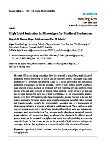
Figure 1: Les 4 étapes de DRUM. Le réseau métabolique est décomposé en sous-réseaux (SN) (étape i) supposés à l’état quasi-stationnaire 𝛼

(étape ii). Ces sous-réseaux sont alors réduits à des réactions macroscopiques (𝑆 → 𝑃) (étape iii), pour lesquelles des cinétiques sont postulées (étape iv). Les métabolites interconnectant les sous-réseaux sont autorisés à s’accumuler (ronds rouges) ou être consommés, ce qui entraine la dynamique de tout le réseau. De l’étape iv), un système d’équations différentielles ordinaires peut être déduit, représentant l’évolution des variables macroscopiques (substrats, biomasse) et les variables intracellulaires (flux métaboliques, métabolites accumulés). Dans le modèle décrit à l’étape i) 𝐾 ∈ ℜ𝑛𝑚 ×𝑛𝑟 , 𝑣 ∈ ℜ𝑛𝑟 , tandis que pour le modèle construit grâce à notre approche, 𝐾′ ∈ ℜ𝑛𝑚′ ×𝑛𝐸 et 𝛼 ∈ ℜ𝑛𝐸 , tels que 𝑛𝑚 ′ ≪ 𝑛𝑚 et 𝑛𝐸 ≪ 𝑛𝑟 .

Application à Tisochrysis lutea soumise à un cycle jour/nuit Afin de valider la méthode DRUM, les données expérimentales d’une culture continue d’ Isochrysis affinis galbana (clone T-iso, CCAP 927/14) soumise à des cycles jour/nuit ont été utilisées (Lacour et al., 2012). Cette microalgue, connue pour accumuler de grandes quantités de lipides, a récemment été renommée Tisochrysis lutea (Bendif et al., 2013). Les cultures ont été réalisées en duplicat dans des réacteurs cylindriques de 5L à température constante (22°). Le pH était régulé à 8.2 grâce à l’injection automatique de CO2. Les mesures suivantes ont été effectuées : nitrates, carbone organique, azote organique, chlorophylle, carbohydrates et lipides neutres (Lacour et al., 2012). La première étape de DRUM consiste à construire le réseau métabolique. Dans le cas de Tisochrysis lutea, comme cette microalgue n’a pas encore été séquencée, aucune reconstruction de réseau métabolique à l’échelle du génome n’est possible. En utilisant les réseaux métaboliques d’autres espèces de microalgues eucaryotes déjà construits (Chlorella pyrenoidosa (Yang et al., 2000), Chlamydomonas reinhardtii (Boyle and Morgan, 2009; Chang et al., 2011; Cogne et al., 2011; Dal’Molin et al., 2011; Kliphuis et al., 2012; Manichaikul et al., 2009), Ostreococcus tauri et Page 27 sur 312

Ostreococcus lucimarinus (Krumholz et al., 2012)), un réseau métabolique cœur, commun à toutes les microalgues, a été déduit. Il comprend les réseaux carbonés centraux tels que la photosynthèse, la glycolyse, la voie des pentoses phosphates, le cycle de Krebs, la phosphorylation oxydative, la synthèse de chlorophylle, de carbohydrates, de lipides, d’acides aminés et de nucléotides. Les chemins métaboliques espèces-spécifiques n’ont pas été représentés car ils ne sont pas connus dans le cas de Tisochrysis lutea et sont supposés négligeables en terme de flux. Conformément à la littérature, les réactions de synthèses des macromolécules (protéines, lipides, ADN, ARN, biomasse) ont été réduites à des réactions génériques où les coefficients stœchiométriques sont déterminés grâce aux données expérimentales (Lacour et al., 2012). Le réseau métabolique ainsi obtenu est composé de 157 métabolites et 162 réactions. Dans une seconde étape, les réactions ont été groupées en sous-réseaux en prenant en compte les fonctions principales du métabolisme. Six sous-réseaux ont été obtenus, correspondant à i) la photosynthèse ii) la glycolyse haute iii) la synthèse de carbohydrates iv) la glycolyse basse v) la synthèse de lipides vi) la synthèse de biomasse (Figure 2). Les métabolites intracellulaires autorisés à accumuler (A) sont, dans ce cas, le phosphoenolpyruvate (PEP), le glyceraldéhyde-3-phosphate (GAP), le glucose-6-phosphate (G6P), les carbohydrates, les lipides et les cofacteurs. Puis, grâce à l’analyse des modes élémentaires, chaque sous-réseau a été réduit à des réactions macroscopiques. En tout, 8 réactions macroscopiques ont été déduites, pour lesquelles des cinétiques proportionnelles simples ont été postulées. Le modèle résultant, composé de 21 métabolites et 8 réactions macroscopiques, possède en tout 10 degrés de liberté, représentés par 10 paramètres cinétiques à déterminer. Ces derniers ont été estimés grâce aux données expérimentales disponibles. Dans des conditions de croissance non-carencée, le modèle prédit avec précision l’accumulation des lipides et des carbohydrates la journée et leur consommation durant la nuit (Figure 3). Le stock de carbone prédit est minimal une heure et demie après le lever du soleil, lorsque la lumière est assez intense pour pouvoir compenser la perte de carbone par respiration (Figure 3D). De manière similaire, les stocks de carbone sont à leur maximum trois heures avant le coucher du soleil, lorsque la lumière ne suffit plus à compenser les pertes générées par la respiration (Figure 3D). Le carbone organique total a un comportement similaire, suggérant de récolter les microalgues en fin de journée, trois heures avant le coucher du soleil, lorsque les lipides sont à leur maximum (Figure 3A et Figure 3D). A midi, lorsque la lumière est à son intensité maximale, le stockage de carbone sous forme de lipides neutres et carbohydrates est également à son maximum. A ce moment, seulement un tiers du carbone entrant dans la cellule est utilisé pour la synthèse de la biomasse. Le reste est stocké sous forme de carbohydrates (37.1%) et de lipides (34.2%) (Figure 4). A la fin de la nuit et au début de la journée, le métabolisme est très ralenti, car très peu de carbone sous forme de Page 28 sur 312

Figure 2 : Réseau métabolique central de Tisochrysis lutea décomposé en six sous-réseaux Les métabolites interconnectant les sous-réseaux sont autorisés à s’accumuler et sont soit situés à l’embranchement de plusieurs chemins métaboliques (glycéraldéhyde-3-phosphate (GAP), glucose-6phosphate (G6P), phosphoénolpyruvate (PEP)), soit des produits finaux du métabolisme (lipides (PA), carbohydrates (CARB), biomasse fonctionnelle (B)), soit des cofacteurs (ATP, ADP,NADH, NAD, NADPH, NADP), soit des métabolites transportés dans la cellule (Light, CO2,O2,Pi,H2O,H,NO3,SO4,Mg). B correspond à la biomasse fonctionnelle qui est composée des protéines, de l’ADN, de l’ARN, de la chlorophylle et des lipides membranaires.

réserve est disponible pour la croissance (Figure 4). Après 24h, le comportement de la microalgue redevient similaire, illustrant la périodicité du métabolisme des organismes photosynthétiques soumis à des cycles jour/nuit (Figure 3 et Figure 4). Enfin, il est intéressant de noter l’évolution des concentrations de PEP, G6P et GAP prédites par le modèle (Figure 3F). Par construction, celles-ci sont négligeables en termes de masse de carbone, montrant que la majorité du stockage du carbone s’effectue avec les lipides neutres et les carbohydrates. Cependant, leurs concentrations ne sont pas constantes dans le temps, et diffèrent particulièrement entre le jour et la nuit, ce qui confère une certaine flexibilité au réseau métabolique lorsque les conditions environnementales changent régulièrement (ici la lumière). Cette flexibilité est liée à certains métabolites, qui agissent comme des «buffers » qui s’accumulent, ce qui n’aurait pas été possible avec une hypothèse de croissance équilibrée. C’est un des avantages clé de l’approche DRUM. Dans le cas d’une carence en azote, le modèle prédit correctement toutes les variables du système sauf les lipides et le carbone organique total qui sont surestimés jusqu’à deux fois plus que ce qui a Page 29 sur 312

Figure 3: Comparaison entre les résultats de simulation et les données expérimentales (noncarencé) A- Evolution de la biomasse totale en termes de carbone organique. modèle ; , données expérimentales ; intensité lumineuse. B- Evolution de la biomasse totale en termes d’azote organique. modèle ; , données expérimentales ; intensité lumineuse C- Evolution de la chlorophylle (supposée fixe par unité de biomasse fonctionnelle. modèle ; , données expérimentales ; intensité lumineuse. D- Evolution des métabolites de stockage d’énergie et de carbone. , , carbohydrates (CARB) ; , , lipides (PA) ; intensité lumineuse. E- Evolution de la biomasse fonctionnelle (protéines, ADN, ARN, chlorophylle, lipides membranaires). modèle ; , données expérimentales ; intensité lumineuse. F- Evolution des métabolites « buffer » situés à l’embranchement de plusieurs chemins métaboliques. glyceraldehyde-3-phosphate (GAP) ; glucose 6-phosphate (G6P) ; phosphoénolpyruvate (PEP); GAP + PEP + G6P ; intensité lumineuse.

Page 30 sur 312

Figure 4 : Flux métaboliques entre les 6 sous-réseaux à différents moments de la journée. Les flux ont été estimés grâce au modèle développé et sont normalisés par moles de carbone produits ou consommés. La largeur d’une flèche représente l’intensité du flux. Au début de la nuit (t=0h), les carbohydrates et lipides sont déjà consommés pour la croissance de la biomasse fonctionnelle. A la fin de la nuit (t=12h), le métabolisme est au ralenti, car les pools de carbones de réserve ont presque été entièrement consommés. A midi (t=18h), lorsque l’intensité lumineuse est à son maximum, un tiers du carbone entrant dans la cellule est utilisé pour la synthèse de biomasse. Le reste est stocké sous forme de carbohydrates (37,1%) et de lipides (34,2%).

été mesuré expérimentalement, malgré la diminution correctement prédite de la concentration de la chlorophylle, et donc de l’absorption des photons entrainant une diminution du flux de carbone inorganique. Plusieurs hypothèses peuvent expliquer cette surestimation du carbone entrainant une surestimation des lipides, dont deux ont été retenues puis testées in silico : i) la diminution de l’entrée en carbone dans la cellule par des mécanismes de régulation ou des chemins dissipatifs au niveau de la photophosphorylation (non représentés jusque-là), ii) l’excrétion de carbone organique dans le milieu sous forme, par exemple, d’exopolysaccharides. La première hypothèse a été implémentée en rendant la cinétique macroscopique d’entrée en carbone dépendante du quota C/N de la cellule. Il a été possible, dans ce cas, de prédire correctement le carbone organique total ainsi que les lipides du système. La seconde hypothèse a été implémentée en ajoutant une réaction de sécrétion au niveau des carbohydrates ou du phosphoenolpyruvate (PEP) ou du glycéraldéhyde-3phosphate (GAP), dont la cinétique est supposée proportionnelle au pool de carbohydrates, PEP ou Page 31 sur 312

GAP présent. Dans ce cas, il n’a pas été possible de prédire correctement le carbone organique total du système, qui reste largement surestimé. Les mêmes sécrétions ont alors été testées avec une cinétique dépendant du ratio C/N de la cellule, comme pour l’hypothèse i). Dans ce cas-là, il a été possible de prédire correctement le carbone organique total ainsi que les lipides. Ainsi, il semblerait qu’une régulation fonction du quota C/N de la cellule soit nécessaire afin de prédire correctement les variables du système, cette régulation ayant une grande importance lors de la carence azotée. Afin de vérifier ces prédictions in silico, une expérience devrait être mise en place, où en plus des mesures effectuées par Lacour et al. en (2012), les mesures d’absorption de lumière par unité de biomasse, l’état des photosystèmes (grâce au PAM), le carbone organique excrété vont être mesurés. Cela permettra de savoir dans quelle mesure des phénomènes d’excrétion et de diminution de l’acquisition du carbone ont lieu. Il est à noter que DRUM a permis, dans ces conditions de culture, de tester diverses régulations à divers endroits du réseau métabolique qui permettent de coller aux données. DRUM a donc permis de révéler des mécanismes de régulation prenant probablement place en condition de carence azotée.

Application à Chlorella sorokiniana en croissance diauxique hétérotrophe sur acétate et butyrate DRUM a également été appliquée à la croissance diauxique hétérotrophe de Chlorella sorokiniana sur acétate et butyrate. Chlorella sorokiniana est une microalgue d’eau fraiche qui peut accumuler de grandes quantités de lipides neutres. C’est donc une espèce prometteuse pour la production de biocarburants. Les données expérimentales utilisées avaient pour vocation d’étudier le couplage possible entre la fermentation sombre et la croissance des microalgues pour produire des biocarburants (biohydrogène et biodiesel) à partir de déchets complexes (déchets ménagers, déchets d’agriculture, digestats, …) (Turon et al., 2014). L’idée était de faire pousser les microalgues sur les effluents issus de la fermentation sombre, principalement composés d’acétate et de butyrate (Rafrafi et al., 2013). Chlorella sorokiniana a poussée en batch dans le noir à différentes concentrations d’acétate (de 0 à 1 g.L-1), de butyrate (de 0 à 1 g.L-1) et à divers mélanges acétate-butyrate (Turon et al., 2014). La température et le pH étaient constants (25°C et pH 6.5), et tous les substrats autres que l’acétate et le butyrate ont été fournis en quantité non-limitantes. Les consommations de l’acétate et du butyrate ont été mesurées par chromatographie gazeuse ; la biomasse a été mesurée par densité optique et en masse sèche (Turon et al., 2014).

Page 32 sur 312

Chlorella sorokiniana n’a pas encore été séquencée. De manière similaire à Tisochrysis lutea en croissance autotrophe, un réseau générique composé des principaux chemins métaboliques d’une microalgue a été utilisé (glycolyse, voies des pentoses phosphates, cycle de Krebs, photosynthèse, synthèses des carbohydrates, des lipides, des protéines, de l’ADN, de l’ARN et de la chlorophylle). La photosynthèse a été supposée non-utilisée, et l’ajout d’un glyoxysome avec les voies de consommation de l’acétate et du butyrate a été effectué, en accord avec la littérature (Caspi et al., 2006; Dal’Molin et al., 2011). La composition de la biomasse ainsi que le terme de maintenance associé à la croissance ont été adaptés en se basant sur des données issues de la littérature (Boyle and Morgan, 2009; Liang et al., 2009). Dans une seconde étape, le réseau métabolique a été découpé en deux sous-réseaux : i) le glyoxysome ii) la synthèse de biomasse. Seul le succinate, métabolite sortant du glyoxysome, a été supposé pouvoir s’accumuler. Grâce aux modes élémentaires, les deux sous-réseaux ont été réduits à 3 réactions macroscopiques. Une réaction représente la conversion de l’acétate en succinate. La seconde représente la conversion du butyrate en acétate, et la troisième correspond à la synthèse de biomasse à partir du succinate. Une cinétique de Michaelis-Menten a été supposée pour la conversion de l’acétate et une cinétique de Haldane augmenté d’un terme d’inhibition par diauxie a été utilisée pour la conversion du butyrate. Enfin, une cinétique linéaire a été supposée pour la formation de biomasse. Le modèle résultant, composé de 12 métabolites et 3 réactions macroscopiques, possède en tout 7 degrés de liberté, représentés par 7 paramètres cinétiques à déterminer. Ces derniers ont été estimés grâce aux données expérimentales disponibles. Le modèle ainsi obtenu a reproduit avec précision les données expérimentales, même pour les données non utilisées pour l’estimation des paramètres (Figure 8-6, Figure 8-5). La croissance diauxique est particulièrement bien représentée, ainsi que la biomasse finale, montrant que les rendements biomasse/substrat ont été bien prédits par la connaissance métabolique (Figure 8-6, Figure 8-5). De manière intéressante, il n’y avait pas de différences dans les distributions relatives de flux métaboliques entre les deux substrats excepté au niveau du transport dans la cellule. Ceci souligne le fait qu’à part sur le transport, probablement aucune autre régulation ne prend part pour adapter le métabolisme à chaque substrat. De plus, il a été montré que le succinate ne se cumulait pas au sein de la cellule. L’hypothèse de croissance équilibrée est donc juste dans ces conditions de croissance. Ainsi, les approches standards de modélisation métaboliques pouvaient être utilisées. Ceci est principalement dû au fait que pour ce type de croissance, le carbone et l’énergie sont liés. Lorsque plus de carbone n’est disponible, plus d’énergie n’est disponible et donc aucun processus intracellulaire ne peut prendre place. Page 33 sur 312

Figure 5: Comparaison entre le modèle et les données expérimentales de la croissance hétérotrophe de Chlorella sorokiniana sur des mélanges d’acétate et de butyrate Les résultats de simulations sont représentés par des lignes tirets (validation du modèle) ou des lignes plaines -1 (estimation du modèle). Les données expérimentales sont représentées par des points. , : acétate (gC. L ) -1 -1 ; , : butyrate (gC. L ) ; , : biomasse (g.L ) -1 -1 A. Croissance sur 0.25 gC.L d’acétate et 0.25 gC.L de butyrate. -1 -1 B. Croissance sur 0.25 gC.L of acétate et 0.5 gC.L de butyrate. -1 -1 C. Croissance sur 0.4 gC.L of acétate et 0.1 gC.L de butyrate. -1 -1 D. Croissance sur 0.5 gC.L of acétate et 0.9 gC.L de butyrate. -1 -1 E. Croissance sur 0.9 gC.L of acétate et 0.1 gC.L de butyrate.

Page 34 sur 312

Figure 6: Comparaison entre le modèle et les données expérimentales de la croissance hétérotrophe de Chlorella sorokiniana sur acétate et butyrate Les résultats de simulations sont représentés par des lignes tirets (validation du modèle) ou des lignes entières -1 (estimation du modèle). Les données expérimentales sont représentées par des points. , : 1 (gC. L ) ; , -1 -1 -1 -1 : 0.5 (gC. L ) ; , : 0.25 (g.L ) ; , : 0.25 (gC.L ) ; , : 0.1 (gC.L ) -1 A. Concentration de la biomasse (g. L ) pour la croissance sur acétate seul. -1 B. Concentration de l’acétate (gC. L ). -1 C. Concentration de la biomasse (g. L ) pour la croissance sur butyrate seul. -1 D. Concentration du butyrate (gC. L ).

L’avantage de DRUM par rapport aux approches de modélisation macroscopiques classiques est que les coefficients stœchiométriques des réactions macroscopiques n’ont pas eu besoin d’être estimés expérimentalement. Ils ont été déduits directement de la connaissance métabolique, leur conférant une justification plus biologique et mécanistique. De plus, DRUM a pour la première permis de prédire en même temps l’échelle macroscopique et intracellulaire de la croissance hétérotrophe des microalgues.

Conclusion & Perspectives La méthode DRUM (Dynamic Reduction of Unbalanced Metabolism), est une nouvelle approche de modélisation métabolique dynamique en croissance non-équilibrée. Celle-ci permet de prédire de manière dynamique l’accumulation de métabolites intracellulaires en utilisant la connaissance du réseau métabolique. La stratégie proposée résulte d’un compromis entre complexité et représentativité. Elle concilie les échelles intracellulaires et macroscopiques dans un environnement fluctuant. Page 35 sur 312

DRUM a été appliquée à la microalgue unicellulaire photoautotrophe Tisochrysis lutea, ce qui a permis de construire un modèle mathématique décrivant l’accumulation des lipides et des carbohydrates chez une microalgue soumise à des cycles jour/nuit. Les résultats obtenus sont en accord avec les données expérimentales, et permettent de mieux appréhender le métabolisme carboné lors du cycle jour/nuit. Le modèle permet également des premiers éléments d’optimisation du bioprocédé. Par exemple, l’efficacité de la production dépendra fortement de l’heure de récolte. De manière générale, DRUM permet de mieux appréhender les mécanismes intracellulaires en jeu au niveau métabolique lorsque le système biologique est soumis à des conditions environnementales fluctuantes. Ceci n’était pas possible avant, car les modèles ne permettaient pas l’accumulation de métabolites intracellulaires. De nombreuses perspectives à ces travaux de thèse peuvent être imaginées. La première consiste à mettre en place la vérification expérimentale des prédictions in silico faites lors de la carence azotée, dans le cas de Tisochrysis lutea. Des améliorations sur certaines parties du réseau métabolique peuvent également être envisagées, telle que l’ajout de différentes classes de lipides ou carbohydrates. Ceci pourrait permettre, par exemple, de prédire les lipides d’intérêt et leurs longueurs de chaine carbonée, car ces derniers ont une influence sur la combustion dans les moteurs (Stansell et al., 2011). De manière plus théorique, des données métabolomiques pourraient permettre de vérifier les hypothèses émises dans le cadre de DRUM, i.e. la non-accumulation au sein de sous-réseaux métaboliques et l’accumulation des métabolites faisant le lien entre ces sousréseaux. D’un point de vue mathématique, une découpe automatique du réseau métabolique en sous-réseaux pourrait être envisagée, en s’appuyant sur les résultats de Flux Coupling Analysis (Marashi et al., 2012), ou en utilisant plus simplement des méthodes de clustering reposant sur la topologie du réseau métabolique (degré des noeuds, gene ontology etc.). La comparaison des résultats d’un modèle construit grâce à DRUM à un modèle cinétique complet (issue de données expérimentales ou artificielles) pourrait également être intéressante afin de valider la méthodologie développée. Enfin, DRUM pourrait être appliqué aux écosystèmes mixtes, afin de mieux comprendre les interactions qui prennent place entre les différentes espèces qui composent la communauté microbienne. En effet, même si l’échelle est différente, les mêmes principes peuvent être utilisés (la compartimentation ayant lieu à une autre échelle entre individus et communautés) pour découper le méta-réseau métabolique.

Page 36 sur 312

Références Bendif, E.M., Probert, I., Schroeder, D.C., Vargas, C. de, 2013. On the description of Tisochrysis lutea gen. nov. sp. nov. and Isochrysis nuda sp. nov. in the Isochrysidales, and the transfer of Dicrateria to the Prymnesiales (Haptophyta). J. Appl. Phycol. 25, 1763–1776. Bernard, O., 2011. Hurdles and challenges for modelling and control of microalgae for CO2 mitigation and biofuel production. J. Process Control 21, 1378–1389. Boyle, N.R., Morgan, J.A., 2009. Flux balance analysis of primary metabolism in Chlamydomonas reinhardtii. BMC Syst. Biol. 3, 1–14. Bro, C., Regenberg, B., Förster, J., Nielsen, J., 2006. In silico aided metabolic engineering of Saccharomyces cerevisiae for improved bioethanol production. Metab. Eng. 8, 102–111. Burgard, A.P., Nikolaev, E. V, Schilling, C.H., Maranas, C.D., 2004. Flux coupling analysis of genomescale metabolic network reconstructions. Genome Res. 14, 301–312. Burgard, A.P., Pharkya, P., Maranas, C.D., 2003. Optknock: a bilevel programming framework for identifying gene knockout strategies for microbial strain optimization. Biotechnol. Bioeng. 84, 647–657. Caspi, R., Foerster, H., Fulcher, C. a, Hopkinson, R., Ingraham, J., Kaipa, P., Krummenacker, M., Paley, S., Pick, J., Rhee, S.Y., Tissier, C., Zhang, P., Karp, P.D., 2006. MetaCyc: a multiorganism database of metabolic pathways and enzymes. Nucleic Acids Res. 34, D511–6. Chang, R.L., Ghamsari, L., Manichaikul, A., Hom, E.F.Y., Balaji, S., Fu, W., Shen, Y., Hao, T., Palsson, B.Ø., Salehi-Ashtiani, K., Papin, J.A., 2011. Metabolic network reconstruction of Chlamydomonas offers insight into light-driven algal metabolism. Mol. Syst. Biol. 7, 1–13. Chisti, Y., 2007. Biodiesel from microalgae. Biotechnol. Adv. 25, 294–306. Cogne, G., Rügen, M., Bockmayr, A., Titica, M., Dussap, C.-G., Cornet, J.-F., Legrand, J., 2011. A modelbased method for investigating bioenergetic processes in autotrophically growing eukaryotic microalgae: application to the green algae Chlamydomonas reinhardtii. Biotechnol. Prog. 27, 631–640. Dal’Molin, C.G.D.O., Quek, L.-E., Palfreyman, R.W., Nielsen, L.K., 2011. AlgaGEM-a genome-scale metabolic reconstruction of algae based on the Chlamydomonas reinhardtii genome. BMC Genomics 12 Suppl 4, 1:10. Dochain, D., 2001. Automatique des bioprocédés. Hermès science publications. Hamilton, J.J., Reed, J.L., 2013. Software platforms to facilitate reconstructing genome-scale metabolic networks. Environ. Microbiol. 16, 49–59. Heijnen, J.J., Verheijen, P.J.T., 2013. Parameter identification of in vivo kinetic models: Limitations and challenges. Biotechnol. J. 8, 768–775. Kim, J., Reed, J.L., 2010. OptORF: Optimal metabolic and regulatory perturbations for metabolic engineering of microbial strains. BMC Syst. Biol. 4, 1–19. Klamt, S., Stelling, J., 2003. Two approaches for metabolic pathway analysis? Trends Biotechnol. 21, 64–69. Kliphuis, A., Klok, A.J., Martens, D.E., Lamers, P.P., Janssen, M., Wijffels, R.H., 2012. Metabolic modeling of Chlamydomonas reinhardtii: energy requirements for photoautotrophic growth and maintenance. J. Appl. Phycol. 24, 253–266.

Page 37 sur 312

Knoop, H., Gründel, M., Zilliges, Y., Lehmann, R., Hoffmann, S., Lockau, W., Steuer, R., 2013. Flux Balance Analysis of Cyanobacterial Metabolism: The Metabolic Network of Synechocystis sp. PCC 6803. PLoS Comput. Biol. 9, 1–15. Krumholz, E.W., Yang, H., Weisenhorn, P., Henry, C.S., Libourel, I.G.L., 2012. Genome-wide metabolic network reconstruction of the picoalga Ostreococcus. J. Exp. Bot. 63, 2353–2362. Lacour, T., Sciandra, A., Talec, A., Mayzaud, P., Bernard, O., 2012. Diel Variations of Carbohydrates and Neutral Lipids in Nitrogen-Sufficient and Nitrogen-Starved Cyclostat Cultures of Isochrysis Sp. J. Phycol. 48, 966–975. Liang, Y., Sarkany, N., Cui, Y., 2009. Biomass and lipid productivities of Chlorella vulgaris under autotrophic, heterotrophic and mixotrophic growth conditions. Biotechnol. Lett. 31, 1043–1049. Mahadevan, R., Schilling, C.H., 2003. The effects of alternate optimal solutions in constraint-based genome-scale metabolic models. Metab. Eng. 5, 264–276. Manichaikul, A., Ghamsari, L., Hom, E., Chin, C., Murray, R., Chang, R., Balaji, S., Hao, T., Shen, Y., Chavali, A., Thiele, I., Yang, X., Fan, C., Mello, E., Hill, D., Vidal, M., Salehi-Ashtiani, K., Papin, J., 2009. Metabolic network analysis integrated with transcript verification for sequenced genomes. Nat. Methods 6, 589–592. Marashi, S.-A., David, L., Bockmayr, A., 2012. On flux coupling analysis of metabolic subsystems. J. Theor. Biol. 302, 62–69. Mata, T.M., Martins, A.A., Caetano, N.S., 2010. Microalgae for biodiesel production and other applications: A review. Renew. Sustain. Energy Rev. 14, 217–232. Orth, J., Thiele, I., Palsson, B., 2010. What is flux balance analysis? Nat. Biotechnol. 28, 245–248. Pharkya, P., Burgard, A., Maranas, C., 2004. OptStrain: a computational framework for redesign of microbial production systems. Genome Res. 14, 2367–2376. Provost, A., Bastin, G., Agathos, S.N., Schneider, Y.-J., 2006. Metabolic design of macroscopic bioreaction models: application to Chinese hamster ovary cells. Bioprocess Biosyst. Eng. 29, 349–366. Rafrafi, Y., Trably, E., Latrille, E., Hamelin, J., Meynial-Salles, I., Benomar, S., Guidici-Orticoni, M.T., Steyer, J.P., 2013. Sub-dominant bacteria as keystone species in microbial communities producing bio-hydrogen. Int. J. Hydrogen Energy 38, 4975–4985. Schuster, S., Dandekar, T., Fell, D.A., 1999. Detection of elementary flux modes in biochemical networks: a promising tool for pathway analysis and metabolic engineering. Trends Biotechnol. 17, 53–60. Segre, D., Vitkup, D., Church, G., 2002. Analysis of optimality in natural and perturbed metabolic networks. Proc. Natl. Acad. Sci. 99, 15112–15117. Shlomi, T., Berkman, O., Ruppin, E., 2005. Regulatory on/off minimization of metabolic flux after genetic perturbations. PNAS 102, 7698–7700. Song, H.-S., Ramkrishna, D., 2009. When is the Quasi-Steady-State Approximation Admissible in Metabolic Modeling? When Admissible, What Models are Desirable? Ind. Eng. Chem. Res. 48, 7976–7985. Spolaore, P., Joannis-Cassan, C., Duran, E., Isambert, A., 2006. Commercial applications of microalgae. J. Biosci. Bioeng. 101, 87–96. Stansell, G.R., Gray, V.M., Sym, S.D., 2011. Microalgal fatty acid composition: implications for biodiesel quality. J. Appl. Phycol. 24, 791–801.

Page 38 sur 312

Turon, V., Baroukh, C., Trably, E., Latrille, E., Fouilland, E., Steyer, J.-P., 2014. Use of fermentative metabolites for heterotrophic microalgae growth: yields and kinetics. Bioresour. Technol. Submitted. Williams, P.J.L.B., Laurens, L.M.L., 2010. Microalgae as biodiesel & biomass feedstocks: Review & analysis of the biochemistry, energetics & economics. Energy Environ. Sci. 554–590. Yang, C., Hua, Q., Shimizu, K., 2000. Energetics and carbon metabolism during growth of microalgal cells under photoautotrophic, mixotrophic and cyclic light-autotrophic/dark-heterotrophic conditions. Biochem. Eng. J. 6, 87–102.

Page 39 sur 312

Introduction Unicellular photoautotrophic microorganisms convert light photons into cell energy and fix carbon dioxide (CO2). These eukaryotes (microalgae) or prokaryotes (cyanobacteria) microorganisms can synthesize many products of industrial interest such as vitamin, polysaccharides, lipids, unsaturated long-chain fatty acids or pigments. These molecules can address different markets in agriculture (food supplement, functional food), cosmetics, health (production of drugs), energy (hydrogen, biodiesel, bioethanol, methane), animal feeding (aquaculture, poultry, pigs), green chemistry (food colorants) or environment (wastewater treatment, CO2 mitigation) (Chisti, 2007; Mata et al., 2010; Spolaore et al., 2006). Initially motivated by the bioenergy potential, phototrophic microorganisms have generated a growing interest due their wide range of possible applications. These photoautotrophic microorganisms mainly require water, light and inorganics nutrients (nitrogen, phosphorus, magnesium, sulfur…) to grow. They were found to grow in very diverse conditions: from freshwater (e.g.: Chlorella vulgaris (Converti et al., 2009)) to hyper salted water (e.g.: Dunaliella salina (Gokhman, 1996)), at negative temperatures (e.g. Chlamydomonas nivalis (Remias et al., 2005)), above 70°C (e.g.: Synechococcus lividus (Meeks and Castenholz, 1971)), at pH lower than 2 (Dunaliella acidophila (Pick, 1999)) to alkaline conditions above pH 10 (e.g.: Arthrospira platensis (Sánchez-Luna et al., 2007). Microalgae and cyanobacteria thus include a very large set of microorganisms and are estimated to be composed from 30000 to several millions different species (Larkum et al., 2012), comprising among others green algae (Chlorophyte), yellow-green algae (Xanthophyta), golden algae (Chrysophyta) and red algae (Rhodophyta) (Koskimaki et al., 2013). In the recent years, with the depletion of oil reserves and the awareness about global warming, these microorganisms have raised interests for their potential to produce renewable energy. Indeed, they can be used to mitigate CO2 from human activities and produce neutral lipids (mainly triglycerides (TAGs)) or starch, which can then be transformed into third-generation biofuels (biodiesel or bioethanol, respectively). One drastic advantage about microalgae and cyanobacteria is their fast growth giving very promising production yields compared to other organisms fixing CO2 as for example high plants (Chisti, 2007). In addition, their capacity to grow in salted waters as well as

Page 41 sur 312

wastewater is particularly interesting, since they do not necessarily compete with agricultural food neither for land nor for water. Even if production yields seem promising, many steps need to be optimized to produce biofuels at the industrial scale at a competitive price and in a sustainable way (Lardon et al., 2009). Mathematical modeling can be of great help for better understanding and optimizing these complex nonlinear biological systems. It can allow to better apprehend the biological mechanisms taking place, to predict production yields of the system, estimate non-measurable variables, estimate some of its parameters and their influence on the performances of the system, optimize the system, act on the system to control it and finally detect abnormalities in the functioning of the bioprocess (Dochain, 2001). Classical modeling approaches of biological systems can be sorted into two main categories: modeling at the macroscopic scale, where microorganisms act as catalysts of macroscopic reactions (Bastin and Dochain, 1990) and modeling at the intracellular scale, which takes into account intracellular mechanisms such as biochemical reactions or genetic regulation (Fell, 1992). Macroscopic models are usually of low dimension. There are well adapted to support online automatic control algorithms. They can predict well the macroscopic scale of bioprocesses such as substrate consumption and biomass growth (Bastin and Dochain, 1990). Unfortunately, the number and nature of the macroscopic reactions necessary to represent the bioprocess, their stoichiometric coefficients and their kinetics need to be determined experimentally (Bernard and Bastin, 2005a, 2005b). In addition, macroscopic modeling does not take into account intracellular mechanisms and can hardly be used for optimization of intracellular molecules of interest. On the other hand, intracellular modeling rely on the knowledge of the biochemical reactions, catalyzed by enzymes, occurring inside the cell. These models are based on the knowledge of the metabolic, transcriptomic and genomic networks. They give a more mechanistic understanding of the cellular behavior and seem more appropriate to describe and optimize bioprocesses implying intracellular molecules. Among the intracellular modeling frameworks, metabolic modeling has proven to be a very efficient tool for optimizing bioproduction. Indeed, in silico study of metabolism helps to better understand the key mechanisms and opens the routes for optimizing the production of molecules of interest. Many examples illustrating how metabolic modeling can help in better understanding and optimizing a bioprocess can be found in literature (Hamilton and Reed, 2013). For example, the in silico study of S. cerevisae metabolism lead to increase up to 25% the production yield of ethanol on xylose/glucose mixtures (Bro et al., 2006).

Page 42 sur 312

However, the use of metabolic models for time varying processes is hampered by the lack of experimental data required to define and calibrate the kinetic reaction rates of the biochemical reactions (Heijnen and Verheijen, 2013). To overcome these hurdles, a commonly used hypothesis is the balanced-growth hypothesis, also called the Quasi-Steady-State Assumption (QSSA). Internal metabolites are assumed not to accumulate inside the microorganisms, which turns out to be a reasonable hypothesis for most of the microorganisms growing under constant conditions. This implies that every substrate uptake leads to growth and product excretion, without accumulation of intermediate compounds. Thanks to this hypothesis, intracellular models are simplified and thus depend only on the stoichiometry of the network, the reaction reversibility and the uptake rate of the substrates. Most of the metabolic modeling and analysis frameworks rely on the balanced-growth hypothesis. These frameworks include: 

Elementary Flux Modes (EFMs) (Schuster et al., 1999) which determines the elemental reactions generating the set of all possible metabolic fluxes,



Flux Coupling Analysis (FCA) (Burgard et al., 2004) which identifies the coupling between metabolic fluxes,



Flux Balance Analysis (FBA) (Orth et al., 2010) which predicts metabolic fluxes distribution in given environmental conditions,



Flux Variance Analysis (FVA) (Mahadevan and Schilling, 2003) which assesses the possible fluxes variability in those conditions,



Gene Deletion Studies (GDS) (Burgard et al., 2003; Kim and Reed, 2010; Pharkya et al., 2004; Segre et al., 2002; Shlomi et al., 2005) which predict the consequences of deleting genes on fluxes distribution.

Overall, these frameworks predict well biomass growth and excreted products synthesis (Edwards et al., 2001; Mahadevan et al., 2002; Song et al., 2009; Zamorano et al., 2013) as long as the balancedgrowth hypothesis is verified (Song and Ramkrishna, 2009a). Metabolic modeling seems very suitable for photoautotrophic microorganisms dedicated to thirdgeneration biofuels since carbohydrates and lipids are the intracellular molecules of interest. However, the balanced-growth hypothesis is unreasonable since they store energy and carbon during the day so as to support growth and maintenance during the night. Their autotrophic metabolism also results in the synchronization of their circadian cycle on the daily light (Mocquet et al., 2013). Therefore, intermediate metabolites such as carbohydrates and lipids accumulate during the day and Page 43 sur 312

are remobilized during the night (Lacour et al., 2012). This periodic behavior cannot be described under the balanced-growth assumption. One way to circumvent this issue is to represent these metabolites as product of the cell during the day and substrate during the night. Therefore, applying one of the above-cited QSSA metabolic modeling frameworks could a priori be possible to represent carbon storage and better understand microalgae metabolism submitted to day/night cycles. In literature, only Knoop et al. [10], using the DFBA framework, computed metabolic fluxes for a full day/night cycle. However, determining an optimization function to represent carbon storage during the day and its consumption during the night is not a trivial task. Indeed, the classical optimization function “maximization of biomass production” does not work: when applying it, all the carbon available will go to biomass synthesis, and none to carbon storage. To circumvent this issue, artificial solutions consist in either forcing fluxes to carbon storage or in forcing the fluxes of biomass synthesis and maintenance (𝐴𝑇𝑃 → 𝐴𝐷𝑃 + 𝑃𝑖 ) and other futile cycles. In their work, Knoop et al. [10], forced fluxes to carbon storage by changing the biomass composition at each time step. Their method indeed predicted metabolic fluxes dynamically but did not allow predicting the fluxes toward carbon storage and hence the dynamic change of biomass composition. Prediction of carbon storage fluxes is essential for better understanding the conditions in which microalgae accumulate more lipids or starch and thus to enhance biofuel production yield. Hence, to model such bioprocesses, a metabolic modeling framework that handles non balanced-growth and dynamics behaviors is necessary. This PhD thesis presents DRUM (Dynamic Reduction of Unbalanced Metabolism), a new metabolic dynamic modeling framework under non-balanced growth. DRUM allows to model dynamically intracellular processes where accumulation of metabolites plays a significant role. DRUM conciliates the macroscopic and metabolic modeling scales: macroscopic reactions are deduced from the metabolic network. It predicts the behavior of macroscopic variables (biomass, substrate consumption,…) as well as metabolic fluxes and accumulation of intracellular metabolites of interest. DRUM was applied to the phototrophic unicellular microalgae Tisochrysis lutea, a microalgae specie with high potential for biofuels production, to represent dynamically the metabolism of a microalgae submitted to day/night cycles in normal and nitrogen starvation conditions. DRUM was also applied to Chlorella sorokiniana to predict metabolic fluxes during heterotrophic diauxic growth on acetate and butyrate. The thesis is composed of nine chapters. The first two chapters introduce the microbial metabolism, and present the existing metabolic modeling frameworks. A reader familiar with metabolism or metabolic analysis may skip these first chapters. The next chapter reviews the existing microalgae Page 44 sur 312

and cyanobacteria metabolic networks. In particular, the influence of light on the metabolism and the way to model it was studied in details. Then a more methodological chapter reviews the mathematical approaches to analyze their metabolism. DRUM, the proposed metabolic modeling framework, is presented in the fifth chapter. The core idea of the approach, its mathematical translation, its assumptions and its justification are discussed. Then, in Chapter 6, DRUM is applied to Tisochrysis lutea submitted to a day/night cycle. Chapter 7 illustrates the application of DRUM in nitrogen starvation and day/night cycles conditions. In Chapter 8, DRUM is applied to the microalgae Chlorella sorokiniana growing in dark conditions on acetate and butyrate. Finally, conclusions and perspectives are discussed in Chapter 9. The results obtained in this thesis were valorized in the following publications: 

Baroukh C, Muñoz-tamayo R, Steyer J, Bernard O, DRUM: a New Framework for Metabolic Modeling under Non-Balanced Growth. Application to the Carbon Metabolism of Unicellular Microalgae, accepted in Plos One



Turon V, Baroukh C, Trably E, Fouilland, E, Steyer, J, Use of fermentative metabolites mixtures for microalgae growth in heterotrophic conditions: yields and kinetics, accepted in Bioresource Technology



Baroukh C, Muñoz-tamayo R, Steyer J, Bernard O, Mathematical modeling of unicellular microalgae and cyanobacteria metabolism for biofuels production, submitted to Current Opinion in Biotechnology



Baroukh C, Muñoz-tamayo R, Steyer J, Bernard O, A state of the art of metabolic networks of unicellular microalgae and cyanobacteria for biofuels production, to be submitted to Metabolic Engineering



Baroukh C, Muñoz-tamayo R, Steyer J, Bernard O, Metabolic Modeling of the Heterotrophic Diauxic Growth of C. Sorokiniana, under writing



Baroukh C, Muñoz-tamayo R, Steyer J, Bernard O, A New Framework for highlighting regulations in metabolic networks. Application to photoautotrophic microalgae submitted to day/night cycles and nitrogen starvation , under writing



Baroukh C, Muñoz-tamayo R, Steyer J, Bernard O, A state of the art of metabolic modeling tools, under writing

The results obtained in this thesis have also been presented in international conferences as listed below:

Page 45 sur 312



Baroukh C, Muñoz-tamayo R, Steyer J, Bernard O, A new framework for metabolic modeling under non-balanced growth. Application to carbon metabolism of unicellular microalgae. Computer Applications in Biotechnology, 2013 (IFAC) – Mumbai, India (keynote presentation)



Baroukh C, Muñoz-tamayo R, Steyer J, Bernard O, A new framework for metabolic modelling under non-balanced growth. Application to photoautotrophic microalgae in day/night cycle. Metabolic Pathway Analysis, 2013 – Oxford, United Kingdom (oral presentation)



Baroukh C, Steyer JP, Bernard O, A new modeling framework: application to microalgae growth, First Young Algaeners Symposium, 2012 – Wageningen, The Nertherlands (poster)

References Bastin, G., Dochain, D., 1990. On-line estimation and adaptive control of bioreactors, Elsevier. Elsevier, Amsterdam. Bernard, O., Bastin, G., 2005a. Identification of reaction networks for bioprocesses: determination of a partially unknown pseudo-stoichiometric matrix. Bioprocess Biosyst. Eng. 27, 293–301. Bernard, O., Bastin, G., 2005b. On the estimation of the pseudo-stoichiometric matrix for macroscopic mass balance modelling of biotechnological processes. Math. Biosci. 193, 51–77. Bro, C., Regenberg, B., Förster, J., Nielsen, J., 2006. In silico aided metabolic engineering of Saccharomyces cerevisiae for improved bioethanol production. Metab. Eng. 8, 102–111. Burgard, A.P., Nikolaev, E. V, Schilling, C.H., Maranas, C.D., 2004. Flux coupling analysis of genomescale metabolic network reconstructions. Genome Res. 14, 301–312. Burgard, A.P., Pharkya, P., Maranas, C.D., 2003. Optknock: a bilevel programming framework for identifying gene knockout strategies for microbial strain optimization. Biotechnol. Bioeng. 84, 647–657. Chisti, Y., 2007. Biodiesel from microalgae. Biotechnol. Adv. 25, 294–306. Converti, A., Casazza, A. a., Ortiz, E.Y., Perego, P., Del Borghi, M., 2009. Effect of temperature and nitrogen concentration on the growth and lipid content of Nannochloropsis oculata and Chlorella vulgaris for biodiesel production. Chem. Eng. Process. Process Intensif. 48, 1146–1151. Dochain, D., 2001. Automatique des bioprocédés. Hermès science publications. Edwards, J.S., Ibarra, R.U., Palsson, B.O., 2001. In silico predictions of Escherichia coli metabolic capabilities are consistent with experimental data. Nat. Biotechnol. 19, 125–130. Fell, D.A., 1992. Metabolic Control Analysis: a survey of its theoritical and experimental development. Biochem. J. 286, 313–330. Gokhman, I., 1996. A Salt-resistant Plasma Membrane Carbonic Anhydrase Is Induced by Salt in Dunaliella salina. J. Biol. Chem. 271, 17718–17723. Hamilton, J.J., Reed, J.L., 2013. Software platforms to facilitate reconstructing genome-scale metabolic networks. Environ. Microbiol. 16, 49–59. Heijnen, J.J., Verheijen, P.J.T., 2013. Parameter identification of in vivo kinetic models: Limitations and challenges. Biotechnol. J. 8, 768–775.

Page 46 sur 312

Kim, J., Reed, J.L., 2010. OptORF: Optimal metabolic and regulatory perturbations for metabolic engineering of microbial strains. BMC Syst. Biol. 4, 1–19. Koskimaki, J.E., Blazier, A.S., Clarens, A.F., Papin, J.A., 2013. Computational Models of Algae Metabolism for Industrial Applications. Ind. Biotechnol. 9, 185–195. Lacour, T., Sciandra, A., Talec, A., Mayzaud, P., Bernard, O., 2012. Diel Variations of Carbohydrates and Neutral Lipids in Nitrogen-Sufficient and Nitrogen-Starved Cyclostat Cultures of Isochrysis Sp. J. Phycol. 48, 966–975. Lardon, L., Helias, A., Sialve, B., Steyer, J., Bernard, O., 2009. Life-cycle assessment of biodiesel production from microalgae. Environ. Sci. Technol. 43, 6475–6481. Larkum, A.W.D., Ross, I.L., Kruse, O., Hankamer, B., 2012. Selection, breeding and engineering of microalgae for bioenergy and biofuel production. Trends Biotechnol. 30, 198–205. Mahadevan, R., Edwards, J.S., Doyle, F.J., 2002. Dynamic flux balance analysis of diauxic growth in Escherichia coli. Biophys. J. 83, 1331–1340. Mahadevan, R., Schilling, C.H., 2003. The effects of alternate optimal solutions in constraint-based genome-scale metabolic models. Metab. Eng. 5, 264–276. Mata, T.M., Martins, A.A., Caetano, N.S., 2010. Microalgae for biodiesel production and other applications: A review. Renew. Sustain. Energy Rev. 14, 217–232. Meeks, J., Castenholz, R., 1971. Growth and Photosynthesis in an Extreme Thermophile, Synechococcus Lividus (Cyanophyta). Arch. Mikrobiol. 78, 25–41. Mocquet, C., Sciandra, A., Talec, A., Bernard, O., 2013. Cell cycle implication on nitrogen acquisition and synchronization in Thalassiosira weissflogii (Bacillariophyceae). J. Phycol. 49, 371–380. Orth, J., Thiele, I., Palsson, B., 2010. What is flux balance analysis? Nat. Biotechnol. 28, 245–248. Pharkya, P., Burgard, A., Maranas, C., 2004. OptStrain: a computational framework for redesign of microbial production systems. Genome Res. 14, 2367–2376. Pick, U., 1999. Dunaliella acidophila-a most extreme acidophilic alga, in: Seckbach, J. (Ed.), Enigmatic Microorganisms and Life in Extreme Environments. Kluwer Academic Publishers, Dordrecht, The Netherlands, pp. 465–478. Remias, D., Lütz-Meindl, U., Lütz, C., 2005. Photosynthesis, pigments and ultrastructure of the alpine snow alga Chlamydomonas nivalis. Eur. J. Phycol. 40, 259–268. Sánchez-Luna, L.D., Bezerra Pedrosa, R., Matsudo, M.C., Sato, S., Converti, A., Monteiro de Carvalho, J.C., 2007. Influence of pH, temperature, and urea molar flowrate on Arthrospira platensis fed‐ batch cultivation: A kinetic and thermodynamic approach. Biotechnol. Bioeng. 96, 702–711. Schuster, S., Dandekar, T., Fell, D.A., 1999. Detection of elementary flux modes in biochemical networks: a promising tool for pathway analysis and metabolic engineering. Trends Biotechnol. 17, 53–60. Segre, D., Vitkup, D., Church, G., 2002. Analysis of optimality in natural and perturbed metabolic networks. Proc. Natl. Acad. Sci. 99, 15112–15117. Shlomi, T., Berkman, O., Ruppin, E., 2005. Regulatory on/off minimization of metabolic flux after genetic perturbations. PNAS 102, 7698–7700. Song, H.-S., Morgan, J.A., Ramkrishna, D., 2009. Systematic development of hybrid cybernetic models: application to recombinant yeast co-consuming glucose and xylose. Biotechnol. Bioeng. 103, 984–1002.

Page 47 sur 312

Song, H.-S., Ramkrishna, D., 2009. When is the Quasi-Steady-State Approximation Admissible in Metabolic Modeling? When Admissible, What Models are Desirable? Ind. Eng. Chem. Res. 48, 7976–7985. Spolaore, P., Joannis-Cassan, C., Duran, E., Isambert, A., 2006. Commercial applications of microalgae. J. Biosci. Bioeng. 101, 87–96. Zamorano, F., Van de Wouwer, A., Jungers, R.M., Bastin, G., 2013. Dynamic metabolic models of CHO cell cultures through minimal sets of elementary flux modes. J. Biotechnol. 164, 409–422.

Page 48 sur 312

Chapter 1 Microbial metabolism in a nutshell This chapter presents the basic principles of cellular metabolism in order to introduce the basic concept of systems biology. This concept of “system” was exploited to define a new metabolic modeling framework that is presented in Chapter 5. 1.1

Introduction ........................................................................................................................... 51

1.2

Energy harvesting .................................................................................................................. 51

1.2.1

Charge

separation

across

a

membrane:

oxidative

phosphorylation

and

photophosphorylation .................................................................................................................. 51 1.2.2 1.3

Direct phosphorylation .................................................................................................. 53

Chemical element assimilation ............................................................................................. 54

1.3.1

Transport ....................................................................................................................... 54

1.3.2

Carbon assimilation ....................................................................................................... 55

1.3.3

Nitrogen assimilation .................................................................................................... 56

1.4

Synthesis of precursor metabolites ....................................................................................... 56

1.4.1

Glycolysis ....................................................................................................................... 57

1.4.2

Pentose Phosphate Pathway ......................................................................................... 58

1.4.3

Tricarboxylic acid cycle .................................................................................................. 59

1.5

Macromolecules and biomass synthesis ............................................................................... 60

1.5.1

Protein synthesis ........................................................................................................... 60

1.5.2

DNA and RNA synthesis ................................................................................................. 61

1.5.3

Carbohydrates synthesis ............................................................................................... 62

1.5.4

Lipids synthesis .............................................................................................................. 63

1.6

A systematic view of metabolism .......................................................................................... 64 Page 49 sur 312

1.7

Enzyme and metabolic regulation ......................................................................................... 65

1.8

Conclusion ............................................................................................................................. 66

References ........................................................................................................................................ 66

Page 50 sur 312

1.1 Introduction Metabolism is the set of life-sustaining chemical reactions taking place inside a living cell. These reactions, catalyzed by enzymes, allow microorganisms to grow and divide. They are organized into sequences called metabolic pathways, in which a chemical compound called metabolite is transformed into another metabolite through several reaction steps. Metabolism can be roughly divided into two categories: 

catabolism, which uses substrates taken from the environment to harvest chemical elements (carbon, nitrogen…) and energy to sustain growth.



anabolism, that uses energy and chemical elements to construct structural components of the cell such as cell walls, proteins, nucleic acids, pigments …

1.2 Energy harvesting Energy in the cell is under the form of small molecules, which allow driving forward thermodynamically unfavorable reactions by donating some of its chemical energy. The key energy molecule present in all living microorganisms is adenosine triphosphate (ATP), formed from adenosine diphosphate (ADP) and inorganic phosphate (Pi). ATP is a universal energy vector, which allows storing the energy lost by exergonic reactions into a practical form, which is thus transported to the endergonic reactions. Even if ATP is common to all forms of life, reactions involved in its synthesis are very diverse. There are two ways of synthesizing ATP: either by establishing a charge separation across a membrane or by taking a phosphate group rich in energy directly from an organic molecule. Other energy vectors exist in the cell, such as NADH, FADH or NADPH. They are commonly called cofactors. The difference with ATP is that their synthesis reactions are oxidoreduction reactions instead of an enzymatic synthesis reaction. NADH is mainly synthesized in glycolysis (Figure 1-4) and in the Tricarboxylic Acid Cycle (TCA cycle). FADH is mainly synthesized in the TCA cycle, and NADPH is synthesized mainly in the pentose phosphate pathway (PPP). These pathways are further detailed in sections 1.4.1, 1.4.2 and 1.4.3. In the following, only ATP synthesis is detailed.

1.2.1 Charge separation across a membrane: phosphorylation and photophosphorylation

oxidative

All living microorganisms are able to establish a charge separation across a cell membrane. It creates an electrochemical potential, which can be converted into chemical energy taking the form of ATP. The electrochemical potential is created by expulsion of protons outside of a membrane. Page 51 sur 312

Accumulation of protons thus creates a positive charge outside the membrane (cathode), whereas a negative charge is present inside the cell (anode). To reestablish balance of charges, protons cross back the membrane through the ATP synthetase enzyme which thus synthesizes ATP from ADP and inorganic phosphate Pi (Figure 1-1).

Figure 1-1: Charge separation across a membrane Adapted from (Perry et al., 2004).

Protons can be directly expulsed from metabolites using membrane proteins. Otherwise, oxidoreduction reactions with an electron donor and a membrane protein can occur, where electrons are transferred from the donor to a membrane protein (flavoproteins, cytochromes, quinones …). Then, the electrons are transferred to other proteins of the same membrane, expulsing protons at each step, until electrons reach a final electron acceptor (Figure 1-2). This sequence of electron transfer is commonly called respiratory chain or oxidative phosphorylation. If the final electron acceptor is oxygen, the organism is said aerobic. Otherwise, the organism is said anaerobic. The electron donors and acceptors can either be organic or inorganic molecules. A particular source of electron is the splitting of water molecules to oxygen thanks to light energy. This process is called photophosphorylation or the light phase of photosynthesis. Microorganisms performing photosynthesis have a light-harvesting system (pigments such as chlorophyll a) collecting photons to a photosystem, which thanks to the energy contained in the photons breaks a molecule of water into oxygen and electrons. Electrons are thus transferred from thylakoid membranes proteins to thylakoid membrane proteins until reaching the NADP electron acceptor, synthesizing NADPH. At each transfer between protein membranes, protons are expulsed to the thylakoid lumen, creating a charge separation. Protons enter back in the chloroplast through the ATP synthetase producing ATP (Figure 1-3). Page 52 sur 312

Figure 1-2: Example of a respiratory chain. Adapted from (Perry et al., 2004).

Figure 1-3: ATP synthesis via photophosphorylation Adapted from (Perry et al., 2004).

1.2.2 Direct phosphorylation Direct phosphorylation corresponds to ATP synthesis thanks to the direct transfer of a phosphate group, rich in energy, of an organic molecule to ADP. This reaction is thus independent of electron transfers and protons gradients.

Page 53 sur 312

One of the most common direct phosphorylation is glycolysis, major catabolic pathway in the cell. From a molecule of glucose and one ATP invested, 2 pyruvate molecules and two ATPs are synthesized (Figure 1-4). Glycolysis is further detailed in section 1.4.1.

Figure 1-4: ATP synthesis via direct phosphorylation in glycolysis Adapted from (Perry et al., 2004).

1.3 Chemical element assimilation Chemical elements must be harvested to support growth. Beside oxygen and hydrogen, which are essential compounds, the main chemical elements composing a living organism are carbon, nitrogen and phosphorus. Other chemical elements can be necessary, such as iron, sulfur, magnesium, particularly for synthesizing some proteins such as membrane proteins. However, they are generally in minor quantities and correspond to secondary metabolism.

1.3.1 Transport Before being assimilated in the metabolism, substrates need to be transported inside the cell. Transport mechanisms commonly found in microorganisms are passive diffusion, facilitated diffusion, active transport and group translocation. Diffusion, whether passive or facilitated, relies on a gradient of concentrations of the molecule to be transported. The molecules pass from the compartment with the higher concentration to the compartment with the lower concentration, until a balance is reached in both compartments.

Page 54 sur 312

Only few molecules are transported inside the cell via passive diffusion, mainly because of the hydrophobic character of the membranes, which are mainly composed of phospholipids. Polar molecules, such as sugars and amino acids cannot cross the membranes with this transport mode. Only water, some alcohols and some fatty acids can passively diffuse. Facilitated diffusion relies on transmembrane proteins called permeases, on which the transported molecules fixe themselves. The proteins thus change their shape to let through the molecule inside the cell. This type of transport does not necessitate any energy. However, permeases only accelerate the diffusion of the molecules inside the cell. There is no possibility to increase concentration in the cell compared to the environment. On the other hand, active transport consumes energy to transport a molecule inside the cell, even if the molecule is less concentrated in the environment. Accumulation of the molecule can thus happen inside the cell. This type of transport relies on transmembrane proteins. Several active transport systems exist, depending on the molecule to be transported and the energy required for that. Metabolites actively transported are certain sugars, amino acids, organic acids and inorganic ions. Finally, group translocation is a transport mechanism requiring several enzymes and where the molecule transported is chemically transformed during the transport. This is the case for the transport of sugars such as glucose, which is transformed to glucose-6-phosphate when transported inside the cell. Eukaryote cells, contrary to prokaryotes, contain organelles with their own non-permeable membranes. Same principles for transport between the different organelles of the cell apply requiring thus an additional energy cost.

1.3.2 Carbon assimilation In heterotrophic mode, carbon is assimilated from a transported organic molecule. In autotrophic regime, inorganic carbon can be assimilated through different pathways. The most studied CO2 assimilating pathway is the Calvin Cycle. This metabolic cycle is decomposed into two steps. The first one corresponds to the incorporation of CO2 thanks to the RuBisCO enzyme from Ribulose-1,5phosphate (RuBP). The second step consists in regenerating RuBP through several enzymatic steps (Figure 1-5). Calvin cycle is used during the often called dark step of photosynthesis. It corresponds to the pentose phosphate pathway in the reductive mode (cf section 1.4.2).

Page 55 sur 312

Figure 1-5: Calvin cycle The black arrow represents the main reaction of the Calvin cycle, which allows assimilating inorganic carbon dioxide in the cell metabolism. The red arrow represents the outcome of the Calvin cycle: a 3-carbons sugar (glyceraldehyde 3-phosphate (GAP)). Arrows thickness represents relative flux values of each reaction for synthesizing a GAP molecule from 3 CO2.

1.3.3 Nitrogen assimilation Nitrogen is a major component in living microorganisms, necessary for proteins and nucleic acids synthesis. Nitrogen is either incorporated from inorganic molecules such as ammonium (NH4+ ), nitrate (NO3-) or N2 or directly from organic molecules such as amino acids. Ammonium is the elemental nitrogen carrier; it is directly assimilated in the metabolism. If the microorganism grows on nitrates or nitrites (NO− 2 ), the nitrogen ions are transported inside the cell and transformed into ammonium before their assimilation into the metabolism. Ammonium is assimilated mainly through two successive reactions: 

Synthesis of glutamate: NH4+ + NADPH + α − ketoglutarate → Glutamate + NADP + H2 O



Synthesis of glutamine: Glutamate + NH4+ + ATP → Glutamine + ADP + Pi + H2 O

1.4 Synthesis of precursor metabolites There exist five principal macromolecules inside the cell of a microorganism: proteins, DNA, RNA, carbohydrates and lipids. These macromolecules are synthesized from a limited number of precursor metabolites, which are synthesized in three main metabolic pathways: glycolysis, the TCA cycle and the pentose phosphate pathway (Figure 1-6, Table 1-1). These pathways are described in detail in the following.

Page 56 sur 312

Figure 1-6: Global view of synthesis and degradation reactions of the cell Adapted from (Perry et al., 2004).

Table 1-1 : List of precursor metabolites for macromolecules synthesis and their origin Metabolite Glycolysis TCA cycle Pentose phosphate pathway cycle Glucose-6-phosphate (G6P) X X Fructose-6-phosphate (F6P) X Ribulose-5-phosphate (R5P) X Erythrose-4-phosphate (E4P) X Glyceraldehyde-3-phosphate X X 3-Phosphoglycerate X Phosphoenolpyruvate X Pyruvate X X Acetyl CoA X X Oxaloacetate X α-ketoglutarate X Succinyl CoA X Taken from (Perry et al., 2004).

1.4.1 Glycolysis Glycolysis is, in most cells, the pathway with the largest flux of carbon. It involves a series of biochemical reactions by which a molecule of glucose is converted to two molecules of pyruvate (PYR). During the sequential reactions of glycolysis, some energy is also released in the form of ATP and NADH. Similar form of glycolysis exists, such as the Entner-Doudoroff pathway or the EmbdenMeyerhof pathway, the latest being presented in details below. Glycolysis usually takes place within the cytosol of the cell, even if it can also occur inside the chloroplast of photoautotrophic microorganisms. The breakdown of glucose into two molecules of pyruvate occurs in ten steps. During the first five reactions, which is called upper glycolysis, the Page 57 sur 312

energy of 2 ATP is invested and the metabolic reactions lead to the formation of glyceraldehyde 3phosphate (GAP) (Figure 1-4). Energy is then released as the two molecules of 1,3bisphosphoglycerate are converted to two molecules of pyruvate in lower glycolysis (Figure 1-4). The net yield is two molecules of ATP per molecule of glucose used. In addition, there is the formation of two molecules of NADH per molecule of glucose, which can create extra ATP thanks to oxidative phosphorylation.

1.4.2 Pentose Phosphate Pathway The major catabolic fate of glucose 6-phosphate (G6P) is glycolytic breakdown to pyruvate. However, G6P can have other catabolic fates, one of which is the pentose phosphate pathway (PPP) to generate either precursor metabolites necessary for macromolecules synthesis such as Ribose-5Phosphate (R5P) or Erythrose-4-Phosphate (E4P) or reductive power under the form of NADPH. During the oxidative phase (Figure 1-7), G6P undergoes oxidation to form R5P and generate two NADPH. When more NADPH is required, the pentose phosphates produced in the oxidative phase of the pathway are recycled into glucose 6-phosphate. In this non-oxidative phase (see Fig. 1.6), R5P and xylulose 5-phosphate (X5P), in a series of rearrangements of the carbon skeletons, are converted to fructose 6-phosphate and glucose 6-phosphate, completing the cycle and allowing continued oxidation of glucose 6-phosphate with production of NADPH.

Figure 1-7: Pentose phosphate pathway Dashed arrows represent precursor metabolites necessary for macromolecules synthesis. Light grey arrows represent metabolic reactions from glycolysis. Black and dark grey arrows represent reactions from the pentose phosphate pathway. Black arrows represent reactions generating NADPH. Arrows’ thickness represents relative fluxes that can be found during heterotrophic growth of Synechocystis sp PCC 6803 on glucose with the model of Shastri et al. (2005).

Depending on the current need of the cell, glucose 6-phosphate will be used in the glycolysis or in the pentose phosphate pathway. For example, when NADPH is forming faster than it is used for biosynthesis, the first enzyme in the pentose phosphate pathway is inhibited and more glucose 6phosphate is available for glycolysis. Page 58 sur 312

1.4.3 Tricarboxylic acid cycle The series of reactions that constitute the citric acid cycle (also known as the tricarboxylic acid cycle, the TCA cycle, or the Krebs cycle) is of central importance in all the living cells. Indeed, this cycle allows producing a number of important precursor metabolites (alpha-ketoglutarate (AKG), oxaloacetate (OA), Succinyl-CoA (SucCoA)) and at the same time it generates energy under the form of the cofactors NADH and FADH. These cofactors can be further transformed into ATP thanks to oxidative phosphorylation. In eukaryotic cells, the TCA cycle occurs in the mitochondria, which also have all necessary enzymes to perform respiration, allowing a direct coupling between the two intracellular pathways. A complete turn of the cycle implies the conversion of one acetyl-CoA and one molecule of oxaloacetate (OA) into two molecules of CO2 and one regenerated molecule of oxaloacetate. Oxaloacetate is in principle never removed; one molecule of oxaloacetate can theoretically convert an infinite number of Acetyl-CoA to CO2. However, some of the intermediate metabolites of the cycle are used for macromolecule synthesis (Table 1-1). These reactions thus exhaust oxaloacetate. To continue the TCA cycle, anaplerotic reactions converting phosphoenolpyruvate (PEP) or pyruvate (PYR) into oxaloacetate are used.

Figure 1-8: The TCA cycle The dashed arrows represent precursor metabolites necessary for macromolecules synthesis. The light grey arrow represents a reaction from glycolysis. The black and dark grey arrows represent reactions belonging to the TCA cycle. Black arrows represent reactions generating energy under the form of ATP or cofactors.

The TCA cycle is the main source of energy in cell growing on six-carbon organic substrate and using cellular respiration for energy synthesis. Indeed, the TCA cycle is the second step in the breakdown of sugars into carbon dioxide and water in order to generate energy. Glycolysis breaks glucose (a sixcarbon-molecule) down into pyruvate (a three-carbon molecule), but releases only a small fraction of Page 59 sur 312

the total available energy of the glucose molecule. The two molecules of pyruvate formed by glycolysis still contain most of the chemical potential energy of glucose, energy that can be extracted in the citric acid cycle. Microorganisms growing on acetate, fatty acids or any other substrate that provides a two-carbons intermediate have a variant version of the TCA cycle called the glyoxylate cycle. It allows, thanks to the glyoxylate shunt composed of the malate synthetase and the isocitrate lyase, to create fourcarbon intermediates (malate and succinate) to generate oxaloacetate so that the TCA cycle is possible.

Figure 1-9: Glyoxylate cycle The dashed arrows represent precursor metabolites necessary for macromolecules synthesis. The black and dark grey arrows represent reactions belonging to the glyoxylate cycle. Black arrows represent reactions generating energy under the form of cofactors.

1.5 Macromolecules and biomass synthesis 1.5.1 Protein synthesis Proteins are composed of amino acid chains and are very abundant in the cell. There exist 20 amino acids composing proteins. There are synthesized by « family », from a limited number of precursor metabolites presented in Table 1-2. Although proteins are obtained by joining the same 20 amino acids in different combinations, they can however perform very different biological functions depending on the exact sequences of amino acids that constitute the chains. Since the role of a protein affects its composition and moreover, some proteins are specific to certain microorganisms, a standard protein composition cannot be established for all living organisms. To represent protein synthesis by a net synthetic reaction involving amino acids, the stoichiometric coefficients should be evaluated for each organism and each type of protein. Page 60 sur 312

Table 1-2: Precursor Metabolites for the synthesis of amino acids grouped by family Family Precursor Metabolite Amino acid Glutamate α- ketoglutarate Glutamate Glutamine Proline Alanine Pyruvate Alanine Valine Leucine Serine 3-Phosphoglycerate Serine Glycine Cystéine Aspartate Oxaloacetate Aspartate Asparagine Methionine Lysine Threonine Isoleucine Aromatics Phosphoenolpyruvate + erythrose-4-phosphate Phenylalanine Tyrosine Tryptophane Histidine 5-Phosphoribosyl-1-pyrophosphate Histidine Taken from (Perry et al., 2004).

1.5.2 DNA and RNA synthesis DNA and RNA (ribonucleic acid), which contains the information necessary to build proteins, are composed of purine and pyrimidine nucleotides. The different purine and pyrimidine nucleotides are illustrated in Figure 1-10. Adenine and guanine are purine nucleotides whereas thymidine, cytosine and uracil (unique to RNA) are pyrimidine nucleotides.

Figure 1-10: Purine and Pyrimidines nucleotides. Page 61 sur 312

The actual biosynthesis of nucleotides is a complex process that proceeds in a different manner for both types of nucleotides. However, their synthesis begins with the same metabolic precursors: aspartate, glutamine, ribose-5-phosphate, CO2, and NH3. The origin of each nuclear element of purines and pyrimidines is exposed in Figure 1-11.

Figure 1-11: Origin of the atoms of purine and pyrimidine nucleotides Taken from (Perry et al., 2004).

1.5.3 Carbohydrates synthesis In microorganisms, carbohydrates are most of the time composed of long chains of six–carbon sugars such as glucose. For example, carbohydrates can be formed from glucose-1-phosphate (G1P) thanks to ATP: 𝑝ℎ𝑜𝑠𝑝ℎ𝑜𝑔𝑙𝑢𝑐𝑜𝑚𝑢𝑡𝑎𝑠𝑒

𝐺1𝑃 ↔ 𝐺6𝑃 { 𝐴𝑇𝑃 + 𝐺1𝑃 → 𝐴𝐷𝑃 − 𝑔𝑙𝑢𝑐𝑜𝑠𝑒 + 𝑃𝑖 (𝑔𝑙𝑢𝑐𝑜𝑠𝑒)𝑛 + 𝐴𝐷𝑃 − 𝑔𝑙𝑢𝑐𝑜𝑠𝑒 → (𝑔𝑙𝑢𝑐𝑜𝑠𝑒)𝑛+1 + 𝐴𝐷𝑃 If not already present in the environment, glucose is synthesized thanks to glycolysis in reverse direction: glyceraldehyde-3-phosphate obtained thanks to the Calvin cycle or lower glycolysis is transformed successively into fructose 1,6-biphosphate (F16P), fructose-6-phosphate (F6P), glucose6-phosphate (G6P) and finally to glucose (Figure 1-12).

Page 62 sur 312

Figure 1-12 : Glucose synthesis. Adapted from (Perry et al., 2004).

1.5.4 Lipids synthesis There exist different types of lipids. They can be roughly divided into three different categories: phospho- and glyco-lipids (constituting membranes), neutral lipids (e.g.: triacylglycerols (TAGs)) and isoprenoids (constituting pigments such as chlorophyll or carotenoids for example). Phospholipids and neutral lipids are usually synthesized from Acetyl-CoA and Malonyl-CoA, which is synthesized itself from carboxylation of Acetyl-CoA (Figure 1-14). Isoprenoids are composed of isoprene units only synthesized from Acetyl-CoA (Figure 1-13).

Figure 1-13 : Biosynthesis of an isoprene unit Adapted from (Perry et al., 2004).

Page 63 sur 312

Figure 1-14 : Synthesis of phospholipids and neutral lipids. Adapted from (Perry et al., 2004).

1.6 A systematic view of metabolism From the description of the main metabolic pathways in sections 1.1-1.5, a notion of “system” emerges. Indeed, microorganisms’ metabolism can be visualized as five primary main functions (Figure 1-15): i) carbon assimilation, ii) nitrogen assimilation iii) assimilation of other chemical elements (phosphate, sulfur, iron, magnesium,…) iv) energy production and v) synthesis of macromolecules to constitute biomass (carbohydrates, lipids, proteins, DNA, RNA,…).In addition, the metabolic network has a bow-tie structure, in which there is a great diversity of inputs (the way chemical elements are assimilated and energy is produced), a great diversity of outputs (carbohydrates, lipids, proteins, DNA, RNA, pigments, vitamins, etc.) but a much smaller diversity in the way the inputs are transformed to outputs, as all metabolites can be produced from 12 key precursor metabolites issued from three metabolic pathways: glycolysis, the pentose phosphate pathway and the TCA cycle.

Page 64 sur 312

Figure 1-15: A systematic view of microorganism metabolic network. Microbial metabolism can be schematically decomposed into: i) carbon assimilation, ii) nitrogen assimilation iii) assimilation of other chemical elements (phosphate, sulfur, iron, magnesium,…) iv) energy production and v) synthesis of macromolecules to constitute biomass (carbohydrates, lipids, proteins, DNA, RNA,…).

1.7 Enzyme and metabolic regulation It must be mentioned that the processes occurring in a cell are much more numerous than those described by the metabolism. Metabolism itself is subject to control. Metabolic regulation can occur when the levels of some metabolites or other substances reach a threshold, when the cell receives a signal, etc. In these cases, the cell adapts itself by taking the proper actions. Metabolic regulation mainly occurs on enzymes, via two types of regulation: i)

Regulation of the quantity of an enzyme, which means regulation at the transcription or translation level. This type of regulation is rather slow, but allows the cell to save energy and nutrients.

ii)

Stimulation or inhibition of the activity of the enzyme. This type of regulation, called posttranslational regulation, is faster and takes place after the synthesis of an enzyme.

The result can be that a metabolic pathway is not used anymore or on the contrary, a new route is triggered. However, the changes can be more subtle. For example, the repartition between two pathways can change. Genomic regulation is complex and regulates metabolic pathways in several other ways.

Page 65 sur 312

Metabolic network describes the flux of mass within the cell. The flux of information is performed by several regulation networks involving mainly genomic, transcriptomic and proteomic regulations … The resulting behavior of the cells results from the interaction between these different mass and information networks.

1.8 Conclusion This chapter presented the basic principles of cellular metabolism and the main metabolic pathways common to most of the microorganisms. The reader can refer to Perry et al. (2004) and Willey et al. (2008) for excellent and more detailed references providing the basics of cellular metabolism. It results that cell are complex dynamical systems, where fluxes of mass, energy and information intricately interact. These fluxes are however structured by specific pathways supporting basic functions and by cell compartmentalization that constraint the set of possible behavior. This notion of nonlinear system has motivated the development of adapted tools derived from the science of dynamical systems. This concept of “dynamical system” was exploited to define the new metabolic modeling framework presented in Chapter 5.

References Perry, J.J., Staley, J.T., Lory, S., 2004. Biosynthèse des monomères, in: Microbiologie, Cours et Questions de Révision. Dunod, Paris, pp. 206–228. Shastri, A.A., Morgan, J.A., 2005. Flux balance analysis of photoautotrophic metabolism. Biotechnol. Prog. 21, 1617–1626. Willey, J., Sherwood, L., Woolverton, C., 2008. Metabolism: Energy, Enzymes, and Regulation, in: Prescott, Harley and Klein’s Microbiology. Mc Graw Hill higher Education, pp. 167–190.

Page 66 sur 312

Chapter 2 Metabolic modeling in a nutshell This chapter is a detailed literature review of the existing metabolic modeling frameworks, their mathematical expression and their use. 2.1

Mathematical representation of metabolism ....................................................................... 69

2.2

Kinetic modeling and the balanced-growth hypothesis........................................................ 71

2.3

Static modeling frameworks.................................................................................................. 73

2.3.1

Elementary Flux Modes ................................................................................................. 74

2.3.2

Flux Coupling Analysis ................................................................................................... 75

2.3.3

Flux Balance Analysis ..................................................................................................... 76

2.3.4

Flux Variance Analysis ................................................................................................... 77

2.3.5

Gene Deletion Studies ................................................................................................... 78

2.4

Dynamical modeling frameworks .......................................................................................... 78

2.4.1

Dynamic Flux Balance Analysis ...................................................................................... 79

2.4.2

Macroscopic Bioreaction Modeling............................................................................... 80

2.4.3

Hybrid Cybernetic Modeling.......................................................................................... 82

2.4.4

Lumped Hybrid Cybernetic Modeling............................................................................ 84

2.5

Conclusion ............................................................................................................................. 87

References ........................................................................................................................................ 87

Page 67 sur 312

2.1 Mathematical representation of metabolism Metabolism of a microorganism can be represented by its metabolic network, which is fully determined by a set of nr biochemical reactions taking the form: 𝑠1 𝑆1 + ⋯ + 𝑠𝑛𝑆 𝑆𝑛𝑆 → 𝑝1 𝑃1 + ⋯ + 𝑝𝑛𝑃 𝑃𝑛𝑃 where 𝑆𝑖 , 1 ≤ 𝑖 ≤ 𝑛𝑠 represents the substrates of the reaction, 𝑃𝑖 , 1 ≤ 𝑖 ≤ 𝑛𝑃 represents the products of the reaction and 𝑠𝑖 , 1 ≤ 𝑖 ≤ 𝑛𝑠 and 𝑝𝑖 , 1 ≤ 𝑖 ≤ 𝑛𝑃 their associated stoichiometric coefficients (Larhlimi et al., 2011). The biochemical reactions can be irreversible (→) or reversible (↔). In general, each reaction is macroscopic and summarizes a set of elemental reactions involving enzymes complexes. As a consequence, the metabolic network (and its size) can vary depending on the description level. Mathematically, a metabolic network is usually represented as a stoichiometric matrix 𝐾 ∈ ℜ𝑛𝑚×𝑛𝑟 where the rows of the matrix correspond to metabolites (𝑛𝑚 in total) and the columns of the matrix correspond to reactions (𝑛𝑟 in total). Metabolites can include both intracellular metabolites and extracellular metabolites such as substrates or excreted products (Figure 2-1). The reactions can thus comprise transport reactions. The coefficients of the matrix are the stoichiometric coefficients of the reactions (Figure 2-1): 

𝐾𝑖,𝑗 = 0 if metabolite i does not participate in reaction j



𝐾𝑖,𝑗 > 0 if metabolite i is a substrate of reaction j



𝐾𝑖,𝑗 < 0 if metabolite i is a product of reaction j

However, in this configuration, reversibility of reactions is not taken into account. To do so, many alternatives are available. For instance, all reversible reactions can be split into two irreversible reactions (a forward and a backward reaction) or the reversibility can be stored into a binary vector 𝑟𝑒𝑣 where 𝑟𝑒𝑣𝑖 = 0 if the reaction is irreversible and 𝑟𝑒𝑣𝑖 = 1 otherwise. Another solution is to store the reversibility into two vectors representing the lower and upper bounds of the reaction flux. If the reaction is reversible, the lower bound is −∝ , otherwise it is 0.

Page 69 sur 312

Figure 2-1: Different representations of metabolic networks: list of reactions, stoichiometric matrix and bipartite graph. A metabolic network can equivalently be represented as a directed weighted bipartite graph composed of two disjoint sets of nodes (reactions and metabolites) and a set of directed and weighted edges between the two types of nodes (Figure 2-1): 

A direct edge is drawn from a metabolite to a reaction if the metabolite is a substrate of the reaction. Its weight is the stoichiometric coefficient.



A direct edge is drawn from a reaction to a metabolite if the metabolite is a product of the reaction. Its weight is the stoichiometric coefficient.

However, in the context of metabolic modeling, this representation is only used to visualize the metabolic network and its flux distribution. For a full review of the representations of metabolic network and their uses, the reader is referred to (Larhlimi et al., 2011). From a computational point of view, a metabolic network can be handled under several file formats, of which the most common are (Figure 2-2): 

1 or 2 CSV or Excel files (one for the stoichiometric matrix, one for the reversibility vector).



A text file with the list of biochemical reactions.



A XML file specifically called SBML in the case of metabolic networks (Hucka et al., 2003).

Page 70 sur 312

Figure 2-2: Different file formats used to encode metabolic networks There is no clear standard and the file format depends on the toolbox or the software used for metabolic modeling and analysis. For example, the COBRA toolbox requires a SBML file, whereas the toolbox efmtool accept SBML files, stoichiometric matrices and list of reactions (Becker et al., 2007; Terzer and Stelling, 2008).

2.2 Kinetic modeling and the balanced-growth hypothesis Kinetic models, also called dynamic models, are usually obtained thanks to a mass-balance, leading to an Ordinary Differential Equation (ODE) system. In the case of metabolism, if the microorganism, grown in a batch reactor, consumes extracellular substrates represented by vector S to synthesize biomass B and excretes products represented by the vector P, and its metabolic network is represented by the stoichiometric matrix 𝐾 ∈ ℜ𝑛𝑚×𝑛𝑟 containing nm metabolites and nr reactions, the ODE system obtained is (Savageau, 1970, 1969a, 1969b): 𝑆 𝐶 𝑑( ) 𝐾𝑆 𝑃 𝑑𝑀 𝐾𝐶 𝐵 = = ( ) . 𝑣. 𝐵 = 𝐾. 𝑣. 𝐵 𝐾𝑃 𝑑𝑡 𝑑𝑡 𝐾𝐵 with 𝑣𝑖 ≥ 0 if 𝑣𝑖 is irreversible, 𝑖 ∈ {1, . . , 𝑛𝑟 }. Page 71 sur 312

(2-1)

where M represents the metabolites concentration vector composed of biomass B, substrates S, intracellular metabolites C and excreted products P. Here, concentrations are expressed in terms of solution concentrations (mM), not concentrations per unit of cell (mM.mM B-1), which is not always the case in literature. In the following, all concentrations will be expressed in mM. The kinetics vector v  nr represents the reactions rates (per biomass unit) of the reactions of the metabolic network;

it is a function of M and of possible environmental variables (temperature, light …). By multiplication to v, biomass B acts as a catalyzer of kinetics v. The matrices 𝐾𝑆 ∈ ℜ𝑛𝑆×𝑛𝑟 , 𝐾𝐶 ∈ ℜ𝑛𝐶 ×𝑛𝑟 , 𝐾𝑃 ∈ ℜ𝑛𝑃 ×𝑛𝑟 and 𝐾𝐵 ∈ ℜ1×𝑛𝑟 are the stoichiometric matrices of the metabolic network for the substrate, the products, the internal metabolites and the biomass (𝑛𝑆 + 𝑛𝐶 + 𝑛𝑃 + 1 = 𝑛𝑚 ). The formulation given in (2-1) requires the kinetic rates functions of each metabolic reaction to be defined, especially to represent the transient dynamics of the set of intracellular compounds. However, the experimental difficulty to measure along time the dynamics of intracellular compounds hampers the modeling and calibration of this large set of kinetics associated to the biochemical reactions of the metabolic network (Heijnen and Verheijen, 2013). A striking example is the failed attempt to model glycolysis using in vitro kinetics, showing the complexity of determining in vivo kinetics (Teusink and Passarge, 2000). To overcome these hurdles, a commonly used hypothesis is the balanced-growth hypothesis, also called the Quasi-Steady-State Approximation (QSSA). Internal metabolites are assumed not to accumulate inside the microorganisms, which turns out to be a reasonable hypothesis for most of the microorganisms growing under constant conditions. This implies that every substrate uptake leads to microbial growth and products excretion. Mathematically, the balanced-growth hypothesis means:

𝐶 𝑑( ) 𝐵 =0 𝑑𝑡 with 𝜇 the biomass growth rate (𝜇 =

𝑑𝐵 ). 𝑑𝑡

⇔

𝑑𝐶 𝑑𝑡

= 𝜇. 𝐶

(2-2)

Dilution by growth (𝜇. 𝐶) is usually neglected (Song et al.,

2009), and system (2-1) can therefore be transformed into: 𝑆 𝑑(𝑃 ) 𝐵 𝑑𝑡

𝐾𝑆 = (𝐾𝑃 ) . 𝑣. 𝐵 𝐾𝐵 {𝐾𝐶 . 𝑣 = 0 with 𝑣𝑖 ≥ 0 if 𝑣𝑖 is irreversible, 𝑖 ∈ {1, . . , 𝑛𝑟 }.. 𝑣 can thus be deduced by solving the system: Page 72 sur 312

(2-3)

𝐾𝐶 . 𝑣 = 0 , 𝑣𝑖 ≥ 0 if 𝑣𝑖 is irreversible, 𝑖 ∈ {1, . . , 𝑛𝑟 }.

(2-4)

Hence, thanks to balanced-growth hypothesis, intracellular models are simplified and depend only on the stoichiometry of the network, the reaction reversibility and the uptake rate of the substrates. However, the dimension of the Kernel of the stoichiometric matrix 𝐾𝐶 is usually not null (𝑛 = dim(𝐾𝑒𝑟𝑛(𝐾𝐶 )) ≠ 0). Hence, there is an infinity of solutions of system (2-4). A method consists in studying the space of solutions of system (2-4), instead of solving it. This led to the development of Flux Coupling Analysis (FCA) (Burgard et al., 2004) and of Elementary Flux Modes Analysis (EFMs) (Schuster et al., 1999) and its associated approaches Macroscopic Bioreaction Models (MBM) (Provost et al., 2006), Hybrid Cybernetic Models (HCM) (Song et al., 2009) and Lumped Hybrid Cybernetic Models (L-HCM) (Song et al., 2012). Another method is to find a way to reduce the number of solutions. For that, two strategies are currently used. The first one consists in using biological knowledge and experimental measurements to make the problem well determined. This was performed, for example, by Cogne et al. (2003) on Arthrospira (spirulina) platensis metabolism. However, this method only works for small metabolic networks with few degrees of freedom (𝑛 < 10), since only a limited number of independent variables can be measured (usually substrate uptake rates, product excretion rates and biomass growth). The second strategy consists in imposing an optimization criterion like maximization of biomass growth. This led to the development of Flux Balance Analysis (FBA) (Orth et al., 2010) and its associated approaches Flux Variance Analysis (FVA) (Mahadevan and Schilling, 2003), Gene Deletion Studies (GDS) (Burgard et al., 2003) and Dynamic Flux Balance Analysis (DFBA) (Mahadevan et al., 2002). In any cases, all the existing metabolic modeling frameworks rely on the balanced-growth hypothesis. The description of each above-cited framework is detailed in the rest of this chapter.

2.3 Static modeling frameworks For the analysis of microbial metabolism under static environmental conditions such as constant substrate consumption rate, mathematical frameworks can roughly be divided into two categories. Some of the modeling frameworks yields quantitative information such as fluxes distributions (FBA, GDS), others yield qualitative information about the global network structure such as its flexibility or robustness (FVA, FCA, EFMs, GDS).

Page 73 sur 312

2.3.1 Elementary Flux Modes The solution set of (2-4), 𝑆𝑠𝑜𝑙 ≝ {𝑣 ∈ ℜ𝑛𝑟 |𝐾𝑐 . 𝑣 = 0 & 𝑣𝑖 ≥ 0 if 𝑣𝑖 is irreversible, 𝑖 ∈ {1, . . , 𝑛𝑟 }}, is a cone, and can be described by a set of elementary vectors called Elementary Flux Modes (EFMs) (Schuster et al., 1999). Indeed, if we define the support of a vector 𝑣 as the set of indices of non-zero element of 𝑣, a set 𝑆𝐸𝐹𝑀 of “non-decomposable” vectors can be found such that any solution 𝑣𝑠𝑜𝑙 ∈ 𝑆𝑠𝑜𝑙 can be written as positive linear combination of elements of 𝑆𝐸𝐹𝑀 : ∀𝑒 ∈ 𝑆𝐸𝐹𝑀 , ∄𝑒 ′ ∈ 𝐶 𝑠𝑢𝑐ℎ 𝑡ℎ𝑎𝑡 𝑆 𝑐 (e′) ≝ {𝑖|𝑒𝑖′ ≠ 0} ⊆ 𝑆 𝑐 (𝑒) ≝ {𝑖|𝑒𝑖 ≠ 0} 𝑛𝐸 and ∀ 𝑣𝑠𝑜𝑙 ∈ 𝑆𝑠𝑜𝑙 , 𝑣𝑠𝑜𝑙 = ∑𝑖=1 𝛼𝑖 𝑒𝑖 = 𝐸𝛼, 𝑒𝑖 ∈ 𝑆𝐸𝐹𝑀 , 𝛼𝑖 ≥ 0, 𝑛𝐸 = 𝑑𝑖 𝑚(𝑆𝐸𝐹𝑀 ), 𝐸 ∈ ℜ𝑛𝑟∗𝑛𝐸 𝑎𝑛𝑑 𝛼 ∈ ℜ+ 𝑛𝐸

(2-5)

Elementary Flux Modes (EFMs) corresponds to non-decomposable steady-state pathways of the metabolic network. The non-decomposability criterion implies that if any of its contributing reaction is deleted, the EFM will not carry a flux under steady-state conditions. Thus the metabolic pathway will not be available for the network and the metabolic function will not be carried out. Elementary Flux Modes therefore corresponds to minimal building blocks of the metabolic network. EFMs allows enumerating all the minimal metabolic capabilities of the microorganism, which makes it a very powerful tool for understanding the microorganism metabolism and can guide for metabolic engineering. Indeed, EFM can be harnessed to know whether a cell is able to produce a metabolite of interest from a given substrate, and at the same time gives the pathways with the maximum production yield (Klamt and Stelling, 2003). In addition, to disable a particular metabolic function, one can disable the EFMs with this function. For that, it is only needed to target one of its reactions, since EFM are non-decomposable. However, since a reaction usually contributes to several EFMs, other metabolic functions might be disabled. Thus a deletion with minimal impact can be found by exploring all the contributing reactions of the EFMs to disable. Several gene deletions studies were implemented using the properties of EFMs as, for example, Minimal Cut Sets (MCS) (Klamt and Gilles, 2004), and their results were successfully tested experimentally (Zanghellini et al., 2013). Another potential application of EFMs is the decomposition property of the solution space 𝑆𝑠𝑜𝑙 . Indeed, a flux distribution 𝑣𝑠𝑜𝑙 solution to (2-4) can be decomposed into the EFM base, which gives the minimal building blocks of the metabolic network that are involved in this flux distribution. However the decomposition into the EFM base is not unique (Rügen et al., 2012). An optimization criterion is necessary to impose a unique decomposition. Several softwares exist to compute elementary flux modes. The most known are metatool (von Kamp and Schuster, 2006) or efmtool (Terzer and Stelling, 2008). In this thesis, the use of efmtool was chosen because of its computation efficiency, which allows the computation of EFM for large Page 74 sur 312

metabolic networks. However, because of the exponential explosion of the number of elementary flux modes with the increase size of the metabolic network, EFMs are difficult to compute for genome-scale metabolic networks (GSMN) (Zanghellini et al., 2013) with a large number of reactions (around 1000). EFMs can be computed so far only on medium-scale metabolic networks (around 200 reactions) (Zanghellini et al., 2013). The concept of extreme pathways (EP) is very close to the concept of EFMs. Indeed, EPs are obtained in a similar way than EFMs, the difference relying in the fact that all reversible reactions are split into two irreversible reactions. However, the solution set has an artificially augmented space (since the reversible reactions are represented as two reactions). This representation constrains the analysis of the metabolic networks and can yield false results such as finding the optimal routes for the production of an excreted product (Klamt and Stelling, 2003; Llaneras and Picó, 2010).

2.3.2 Flux Coupling Analysis Flux Coupling Analysis (FCA) allows detecting dependencies between reaction fluxes of metabolic networks at QSSA (Burgard et al., 2004). Indeed, the stoichiometric and other constraints not only determine all possible steady-state flux distributions over a network, they also induce coupling relations between the reactions. For example, if a flux through a reaction in steady-state implies a flux through another reaction, then the two reactions are said to be coupled. There are several types of flux coupling (Larhlimi et al., 2012b): Definition 2-1: Blocked reaction Let 𝑖 ∈ {1, … , 𝑛𝑟 } be a reaction. If 𝑣𝑠𝑜𝑙,𝑖 =0, for all 𝑣𝑠𝑜𝑙 ∈ 𝑆𝑠𝑜𝑙 , reaction 𝑖 is said blocked. Otherwise 𝑖 is unblocked. Definition 2-2: Coupling relations Let 𝑖, 𝑗 ∈ {1, … , 𝑛𝑟 } be two unblocked reactions. The (un)coupling relationships 𝑖 → 𝑗, 𝑖 ↔ 𝑗, 𝑖 ⇔ 𝑗, 𝑈𝐶

and 𝑖 ↔ 𝑗 are defined in the following way: 

𝑖 is directionally coupled with 𝑗, noted 𝑖 → 𝑗, if for all 𝑣𝑠𝑜𝑙 ∈ 𝑆𝑠𝑜𝑙 , 𝑣𝑖 = 0 ⟹ 𝑣𝑗 = 0



𝑖 is partially coupled with 𝑗, noted 𝑖 ↔ 𝑗, if 𝑖 → 𝑗 & 𝑗 → 𝑖



𝑖 is fully coupled with 𝑗, noted 𝑖 ⇔ 𝑗, if 𝑖 ↔ 𝑗 and there exist a constant 𝜆 such that ∀𝑣𝑠𝑜𝑙 ∈ 𝑆𝑠𝑜𝑙 , 𝑣𝑗 = 𝜆𝑣𝑖



𝑈𝐶

𝑖 is uncoupled to 𝑗, noted 𝑖 ↔ 𝑗 , if neither 𝑖 → 𝑗 nor 𝑗 → 𝑖 holds.

Page 75 sur 312

FCA has been used for exploring various biological questions such as network evolution, gene essentiality, gene regulation or analysis of experimentally measured fluxes (Larhlimi et al., 2012b). Indeed, on the one hand, FCA can help in the curation of reconstructed metabolic networks by verifying whether the coupling between reactions is in agreement with the experimental findings. On the other hand, FCA can help in defining intervention strategies to knock out target reactions. Several toolboxes exist to perform FCA. The most recent ones, which allows the computation of FCA for genome-scale metabolic networks, are FFCA and F2C2 (David et al., 2011; Larhlimi et al., 2012b).

2.3.3 Flux Balance Analysis As explained in section 2.2, the solution of (2-4) is not unique and often infinite. To get a smaller set of solutions, an optimization criterion can be used (Orth et al., 2010). The most common optimization criterion is the maximization of biomass growth. Hence the equation system (2-4) becomes: 𝑜𝑏𝑗 = 𝑀𝑎𝑥𝑖𝑚𝑖𝑧𝑒(𝑣𝑏𝑖𝑜𝑚𝑎𝑠𝑠 ) such that {𝐾𝑣 = 0 𝑣𝑖 ≥ 0 𝑓𝑜𝑟 𝑖𝑟𝑟𝑒𝑣𝑒𝑟𝑠𝑖𝑏𝑙𝑒 𝑣𝑖

(2-6)

To further reduce the solutions space and better understand metabolism in specific environmental conditions, additional constraints can be added to (2-6) such as maximum flux rates, experimentally measured fluxes (𝑚𝑠 ) or thermodynamic constraints. The system (2-6) thus becomes: 𝑜𝑏𝑗 = 𝑀𝑎𝑥𝑖𝑚𝑖𝑧𝑒(𝑣𝑏𝑖𝑜𝑚𝑎𝑠𝑠 ) such that 𝐾𝑣 = 0 𝑙𝑜𝑤𝑒𝑟 𝑏𝑜𝑢𝑛𝑑 < 𝑣𝑖 < 𝑢𝑝𝑝𝑒𝑟 𝑏𝑜𝑢𝑛𝑑 { 𝑣𝑆 = 𝑚𝑠

(2-7)

Several others optimization criteria can sometimes be found in literature. There are non-linear objective functions such as maximization of the biomass yield (𝑀𝑎𝑥𝑖𝑚𝑖𝑧𝑒(𝑣𝑏𝑖𝑜𝑚𝑎𝑠𝑠 /𝑣𝑔𝑙𝑢𝑐𝑜𝑠𝑒 )) (Schuetz et al., 2007) or multi-objectives functions such as minimizing total overall fluxes and maximizing biomass yield (𝑀𝑖𝑛𝑖𝑚𝑖𝑧𝑒(∑ 𝑣) 𝑎𝑛𝑑 𝑀𝑎𝑥𝑖𝑚𝑖𝑧𝑒(𝑣𝑏𝑖𝑜𝑚𝑎𝑠𝑠𝑒 /𝑣𝑔𝑙𝑢𝑐𝑜𝑠𝑒 )) (Schuetz et al., 2012). The choice of the objective function depends on the available data, the constraints imposed, and the aim of the model. For example, if biomass growth is measured, the biomass flux 𝑣𝑏𝑖𝑜𝑚𝑎𝑠𝑠 can be constrained to the measured growth rate. Hence, the objective function will not be to maximize the biomass growth. It will be, for example, the minimization of substrate consumption. If substrate consumption was also measured, 𝑣𝑠𝑢𝑏𝑠𝑡𝑟𝑎𝑡𝑒 can be constrained to the measured value and the objective function can become minimization of ATP utilization, or minimization of overall flux values. In this case, for example, the model can be used for estimating maintenance terms (growth associated and non-growth associated) (Kliphuis et al., 2012). But if the model was intended to Page 76 sur 312

predict biomass growth, the objective function will be maximization of biomass growth and model prediction of 𝑣𝑏𝑖𝑜𝑚𝑎𝑠𝑠 will be compared to measured growth rate to validate the model. It is worth noting that the FBA solution is the EFM with the best yield, in the case of a linear objective function corresponding to the maximization of a product or biomass (Klamt and Stelling, 2003). Flux Balance Analysis can thus be used to predict fluxes distributions of intracellular reactions in given environmental conditions. FBA is a widely used approach and one of the few approaches that can be used on genome-scale metabolic networks (GSMN). FBA can, by extension, also be used to compare fluxes between different environmental conditions of different species. The impact of a given reaction on the objective function, whether its flux is diminished (inhibition), highly increased (catalyze) or deleted (gene deletion) can be also studied to help designing new strains. Several software to compute Flux Balance Analysis exist, of which the most known is the COBRA toolbox available for Matlab (Becker et al., 2007). However, any computing language can be used since only an optimization toolbox is necessary to perform FBA.

2.3.4 Flux Variance Analysis In FBA, even if an optimization criterion is applied to get one solution of system (2-4), the solution is often not unique. Several optimal flux distributions can be found. To explore all the possible optimal flux distributions, Flux Variance Analysis (FVA) can be used (Mahadevan and Schilling, 2003). For that, once the optimal value of the objective function 𝑓𝑜𝑝𝑡 has been found, each flux are maximized and minimized to get the range of values that each flux can take that are consistent with (2-7): 𝑜𝑏𝑗2 = 𝑀𝑎𝑥𝑖𝑚𝑖𝑧𝑒(𝑣𝑘 ) 𝑜𝑟 𝑀𝑖𝑛𝑖𝑚𝑖𝑧𝑒(𝑣𝑘 ) such that 𝐾𝑣 = 0 𝑙𝑜𝑤𝑒𝑟 𝑏𝑜𝑢𝑛𝑑 < 𝑣𝑖 < 𝑢𝑝𝑝𝑒𝑟 𝑏𝑜𝑢𝑛𝑑 ∀𝑣𝑘 : 𝑣𝑆 = 𝑚𝑠 {𝑜𝑏𝑗 = 𝑓𝑜𝑝𝑡

(2-8)

FVA allows to find the parallel optimal routes of the metabolic network and to better understand the robustness of the network. Indeed, biological systems often have redundant parallel pathways which carry the same functional purpose. These redundancies contribute significantly to the robustness of the metabolic network in the context of optimal growth and lead to alternate optimal flux distributions. Some reactions can be found optional if they can carry a null flux in an optimal flux distribution. Others can be found essential if they always carry a non-null flux. However, we need to keep in mind the fact that these results are highly dependent on the constraints used and the choice of the optimal function for the FBA solution.

Page 77 sur 312

FVA can be computed thanks to several software, including the COBRA toolbox available for Matlab (Becker et al., 2007). However, any computing language can be used since only an optimization toolbox is necessary.

2.3.5 Gene Deletion Studies Gene deletion studies (GDS) exploit the Gene-Enzyme-Reaction relationship to predict the effect of the deletion of a gene or several genes on the growth and/or on product synthesis. Indeed, by construction, most of the reactions of metabolic network are linked to its enzyme(s), which are, in their turn, linked to its encoding gene(s). Gene knockout results in deletion of the corresponding reaction(s) in the metabolic network, on which metabolic modeling framework (usually FBA) can be applied and results can be compared to the ones obtained for the wild type strain. In a similar way, gene addition studies can be performed to know the impact of the addition of a gene and hence the addition of a metabolic reaction on the growth of the microorganisms and the synthesis of a product of interest. However, for large metabolic networks, systematic deletion of all possible combinations of genes to optimize the production of a molecule of interest requires a daunting amount of computing time. To overcome this hurdle, some gene deletion studies frameworks have been proposed: OptKnock (Burgard et al., 2003), OptGene (Patil et al., 2005), OptStrain (Pharkya et al., 2004), OptORF (Kim and Reed, 2010), OptReg (Pharkya and Maranas, 2006), MOMA (Segre et al., 2002), ROOM (Shlomi et al., 2005), Stoichiometric Capacitance (Larhlimi et al., 2012a) … These frameworks allow to guide in silico gene knockouts in a systematic and biologically meaningful way. The reader is referred to Chan et al. (2013) for a full review of metabolic in silico gene deletions studies.

2.4 Dynamical modeling frameworks The previously detailed metabolic frameworks are all static. To represent the unsteady behavior of the metabolism, a dynamical modeling framework is necessary. A number of them were already developed, all relying on system (1-3). These frameworks include Dynamical Flux Balance Analysis (DFBA) (Mahadevan et al., 2002), Macroscopic Bioreaction Models (MBM) (Provost et al., 2006), Hybrid Cybernetic Models (HCM) (Song et al., 2009) and Lumped Hybrid Cybernetic Models (L-HCM) (Song et al., 2012). Thanks to elementary flux mode analysis, the solution of ( K C .v  0 and𝑣 ≥ 0 if v is irreversible) can be reduced to a set of macroscopic reactions (Klamt and Stelling, 2003; Provost et al., 2006; Song and Ramkrishna, 2009a) :

Page 78 sur 312

𝑣 = 𝐸. 𝛼 𝛼 ≥ 0 𝛼 (𝐾𝑆 . 𝐸). 𝑆 → (𝐾𝑃 . 𝐸). 𝑃 + (𝐾𝐵 . 𝐸). 𝐵

(2-9)

where E is the matrix of elementary flux modes (EFM) and α is the weight vector of the EFM. α can be interpreted as the kinetics of the macroscopic reactions described by the stoichiometric matrix 𝐾𝑆 . 𝐸 𝐾 ′ = (𝐾𝑃 . 𝐸 ) (Song and Ramkrishna, 2009a). The equation system (2-3) can thus be simplified to: 𝐾𝐵 . 𝐸 𝑆 𝑑(𝑃 ) 𝐵 𝑑𝑡

𝐾𝑆 𝐾 = ( 𝑃 ) . 𝐸. 𝛼. 𝐵 = 𝐾 ′ . 𝛼. 𝐵, with 𝛼 ≥ 0 𝐾𝐵

(2-10)

with K’ a new stoichiometric matrix representing the macroscopic reactions and α their kinetics. Hence to predict dynamically metabolic fluxes, only the kinetics α need to be postulated. This is a delicate task, and unfortunately there is no unique or systematic way of doing it. The choice is left to the researcher’s attention and experience and is also relative to the experimental data available. Classical kinetics found in literature are mass-action, power-law, Michaelis-Menten, Hill, cybernetic kinetics (Young and Ramkrishna, 2007). The limitation of this approach, however, is the combinatorial explosion of the number of Elementary Flux Modes when the size of the metabolic network is large. This results in a high number of kinetics α that need to be postulated. Therefore, the dynamic reduction (QSSA) does not imply a reduction of the model dimension. Each existing dynamic metabolic network brings a solution to this problem. Indeed, the Dynamical Flux Balance Analysis (DFBA) approach consists in choosing only a set of EFMs using an optimization framework (Mahadevan et al., 2002). Macroscopic Bioreaction Models (MBM) (Provost et al., 2006) reduces the number of EFMs using experimental data. Hybrid Cybernetic Models (HCM) (Song et al., 2009) reduces the number of EFM by projection of the modes into the yield space. Finally, another solution consists in grouping EFMs into clusters and creating an average EFM for each cluster. This approach is used in the Lumped Hybrid Cybernetic Models (L-HCM) (Song et al., 2012). Overall, these frameworks predict well biomass growth and excreted products synthesis (Edwards et al., 2001; Mahadevan et al., 2002; Song et al., 2009; Zamorano et al., 2013) as long as the balanced-growth hypothesis is verified (Song and Ramkrishna, 2009a).

2.4.1 Dynamic Flux Balance Analysis Dynamic Flux Balance Analysis (DFBA) is a dynamic extension of Flux Balance Analysis (FBA) (Mahadevan et al., 2002). As for FBA, the optimization of an objective function allows reducing the number of solutions in choosing only a subset of them, represented by a subset of EFMs. DFBA

Page 79 sur 312

consist in dividing the time period into N time intervals and solving an FBA at each time interval, followed by integration over the interval of the solution. DFBA mathematically translates to: At each time step 𝑡 ∈ [𝑡0 ; 𝑡𝑓 ], solve: 𝑜𝑏𝑗 = 𝑀𝑎𝑥𝑖𝑚𝑖𝑧𝑒(𝑣𝑏𝑖𝑜𝑚𝑎𝑠𝑠 (𝑡)) such that 𝐾𝑣 = 0 {𝑙𝑜𝑤𝑒𝑟 𝑏𝑜𝑢𝑛𝑑 < 𝑣𝑖 < 𝑢𝑝𝑝𝑒𝑟 𝑏𝑜𝑢𝑛𝑑 𝑣𝑆 (𝑡) = 𝑚𝑠 (𝑡) then compute: 𝑆(𝑡 + 𝑑𝑡) (𝑃(𝑡 + 𝑑𝑡)) = 𝐾. 𝑣(𝑡). 𝑑𝑡 𝐵(𝑡 + 𝑑𝑡)

(2-11)

The optimization problem can be solved using Linear Programming, as for FBA. DFBA was implemented in the COBRA Matlab toolbox (Becker et al., 2007).

2.4.2 Macroscopic Bioreaction Modeling Macroscopic Bioreaction Models (MBM) (Provost et al., 2006) consist in reducing the number of EFMs using experimental data. Indeed, during a specific growth phase, some of the external metabolites consumption or production rate are constant by biomass unit and can be experimentally 1 𝑑𝑀𝑚𝑒𝑠 𝐵 𝑑𝑡

measured (

= 𝑐𝑠𝑡𝑒 = 𝑣𝑚𝑒𝑠 with Mmes consisting of substrates S, products P or biomass B). Let

us denote 𝑣𝑚𝑒𝑠 ∈ ℜ𝑛𝑚𝑒𝑠 the vector of the measured consumption or production rate, where nmes represents the number of metabolites measured: 1 𝑑𝑀𝑚𝑒𝑠 ′ = 𝑐𝑠𝑡𝑒 = 𝑣𝑚𝑒𝑠 = 𝐾𝑀𝑚𝑒𝑠 . 𝑣 = 𝐾𝑀𝑚𝑒𝑠 . 𝐸. 𝛼 = 𝐾𝑀 .𝛼 ,𝛼 ≥ 0 𝑚𝑒𝑠 𝐵 𝑑𝑡

(2-12)

The equation system (2-12) is equivalent to: 𝛼 (𝐾𝑀𝑚𝑒𝑠 . 𝐸 − 𝑣𝑚𝑒𝑠 ). ( ) = 0 1

(2-13)

As for the definition of EFM, any solution of equation (2-13) can be written as a positive linear combination of elementary vectors 𝐻 ∈ ℛ (𝑛𝐸 +1)×𝑛𝐻 : 𝛼 ( ) = 𝐻. 𝛽, 1

𝛽≥0

(2-14)

Hence if we note 𝐻 ′ = 𝐻1:𝑛𝐸 ,1:𝑛𝐻 the sub-matrix of H without the last row, 𝛼 = 𝐻 ′ . 𝛽 and system (2-10) can be reduced to: 𝑆 𝑑(𝑃 ) 𝐵 𝑑𝑡

= 𝐾 ′ . 𝛼. 𝐵 = 𝐾 ′ . 𝐻 ′ . 𝛽. 𝐵 = 𝐾 ′′ . 𝛽. 𝐵 with 𝛽 ≥ 0

Page 80 sur 312

(2-15)

with K’’ a new stoichiometric matrix representing the macroscopic reactions in accordance with experimental data and β their kinetics. Hence only the kinetics β need to be postulated. It is to be noted that the decomposition β is not unique for a solution of (2-14). The model (2-15) can be viewed as a reduction of (2-10) using experimental data (Figure 2-3). Similarly to EFMs (that represent minimal metabolic pathways), 𝐻 ′ represents minimal flux distribution in accordance with experimental measurements.

Figure 2-3: Cone of flux distribution The cone of flux distribution H’ is embedded into the cone the Elementary Flux Modes E. The cone of flux distribution H’ is thus a reduction of the cone E, thanks to experimental data.

However, the necessity to have a fixed measured rate by biomass unit limits the application of this method. Nevertheless, a dynamic metabolic behavior can be decomposed into several time phases during which some external metabolites have a constant consumption or production rate by biomass unit. The method can thus be applied to each phase, and the transition between the phases can be performed thanks to smooth switching functions (Provost et al., 2006). For example, if the biological system undergoes three different metabolic phases (e.g.: growth phase (g), transition phase (t) and death phase (d)), one model can be obtained for each phase and the resulting three equations systems can be merged into one as follows: 𝑆 𝑑 (𝑃 ) 𝐵 = Φ 𝐾′′ . 𝛽 . 𝐵 + Φ 𝐾′′ 𝛽 . 𝐵 + Φ 𝐾 ′′ 𝛽 . 𝐵 𝑔 𝑔 𝑔 𝑡 𝑡. 𝑡 𝑑 𝑑. 𝑑 𝑑𝑡

(2-16)

with Φ𝑔 , Φ𝑡 and Φ𝑑 smooth switching functions which are functions of time and whose value is 1 when the phase is active, 0 when the phase is inactive and varies from 0 to 1 during the transition between the inactive state and the active state (Figure 2-4). Yet, a thorough analysis of experimental data is necessary to determine the metabolic phases and the time window of the transitions between each phase.

Page 81 sur 312

Figure 2-4: The smooth switching functions. Taken from (Provost et al., 2006).

2.4.3 Hybrid Cybernetic Modeling Hybrid Cybernetic Modeling (HCM) consists in assuming cybernetic kinetics for the vector α in (2-10) (Song et al., 2009) (Figure 2-5). Cybernetic kinetics consists of classic Michaelis-Menten kinetics catalyzed by an enzyme e with in addition regulatory terms implemented thanks to cybernetic variables u and v. Indeed, the kinetic 𝛼𝑖 = 𝑓(𝑆1 , … , 𝑆𝑛 ) of a macroscopic reaction 𝑖 with substrates 𝑆1 , … , 𝑆𝑛 can be written as: 𝛼𝑖 = 𝑣𝑖 ∗ 𝑒𝑖 ∗ 𝜇𝑚𝑎𝑥,𝑖 ∗

𝑆1 𝑆𝑛 ∗ … ∗. 𝐾𝑠,𝑆1 + 𝑆1 𝐾𝑠,𝑆𝑛 + 𝑆𝑛

(2-17)

with vi the cybernetic variable controlling the activity of enzyme ei, µmax,i the maximum uptake rate without enzyme regulation and Ks,S1, …, Ks,Sn the demi-saturation constants for each substrate S1,…,Sn. The dynamics of enzymes ei are described thanks to: 𝑑𝑒𝑖 𝑒𝑖 = 𝐴𝑖 + 𝑢𝑖 ∗ 𝜇𝑚𝑎𝑥,𝑒𝑖 ∗ − 𝐷𝑖 ∗ 𝑒𝑖 − 𝜇 ∗ 𝑒𝑖 𝑑𝑡 𝐾𝑠,𝑒𝑖 + 𝑒𝑖

(2-18)

with Ai the basal enzyme synthesis rate, ui the cybernetic variable controlling the enzyme synthesis activity, µmax,ei the maximum enzyme synthesis rate without regulation, Ks,ei the demi-saturation constant, Di the degradation rate and 𝜇 ∗ 𝑒𝑖 represents dilution by growth.

Page 82 sur 312

Figure 2-5: Schematic representation of the Hybrid Cybernetic Modeling concept Taken from (Song et al., 2009)

The cybernetic variables ui and vi describe the regulatory mechanisms modulating enzyme synthesis and their activities, respectively. A general form of ui and vi can be given as follows: 𝑢𝑖 =

𝑝𝑖+

(|𝑝1+ | + ⋯ + |𝑝𝑛+𝐸 |) 𝑝𝑖+ 𝑣𝑖 = max(𝑝1+ , … , 𝑝𝑛+𝐸 ) with 𝑝𝑖+ = max(𝑝𝑖 , 0)

(2-19)

with pi the return-on-investment associated with the ith macroscopic reaction. Determination of pi requires the specification of a metabolic objective function that a cell may try to maximize towards ensuring survival. The most used one is biomass growth, as for FBA. Substrate uptake rates have also been used as an objective function (Song et al., 2009). In this case, for example, pi is expressed as: 𝑝𝑖 = 𝑛𝑏(𝐶) ∗ 𝑒𝑖 ∗ 𝜇𝑚𝑎𝑥,𝑖

(2-20)

with 𝑛𝑏(𝐶) the number of carbon element contained in the substrates consumed through EFM i. To summarize, for each EFM i, a cybernetic kinetic αi is postulated, for which at least 6 parameters need to be estimated (𝜇𝑚𝑎𝑥,𝑖 , 𝐾𝑆,𝑆𝑗 , 𝐴𝑖 , 𝐷𝑖 , 𝜇𝑚𝑎𝑥,𝑒𝑖 , 𝐾𝑆,𝑒𝑖 ). A summary of the approach is described in Page 83 sur 312

Figure 2-5. The drawback of representing enzyme and regulation levels, is that it leads to a very high number of parameters which are often hard to estimate. It often results in an over-parameterization of the model with respect to the available measurements. As a result, most of the parameters are assumed to have basic values such as 0.2 for 𝐾𝑠 coefficients and have limited impact on the model predictions (Song and Ramkrishna, 2012). The application of the cybernetic approach is prohibited for genome-scale metabolic networks described by a high number of EFMs. Hence a reduction of EFMs might be necessary to apply this method. For that, Song et al. (2009b) proposed to reduce the number of EFMs by projecting them into the yield space (Figure 2-6). The method is called Yield Analysis (YA). The yield space is the space of yields of extracellular metabolites of interest. For example, if a microorganism consumes substrate S to produce product P and biomass B, the yield space is a 2-D space composed of biomass B and product P yields with respect to substrate S. Projection of the EFMs in the yield space results in a convex bounded hull, instead of an unbounded polyhedral cone as in the flux space. The convex bounded hull can be defined by its vertices, corresponding to a subset of EFMs, which are called Generating Modes (GMs). Their number is thus smaller than the number of EFMs. An additional reduction can be made by finding the GMs taking into account only a percentage of the convex bounded hull in the yield space (99% of the volume usually). Once the GMs are determined, HCM can be applied to them.

Figure 2-6: Yield Analysis The EFMs are projected into the yield space. A convex bounded hull is obtained. The EFMs are reduced to its vertices composed of a subset of EFMs, which are called Generating Modes (GMs). The number of EFMs is thus largely reduced.

2.4.4 Lumped Hybrid Cybernetic Modeling Even if Yield Analysis is performed, this might not be sufficient enough to reduce the number of EFMs for which kinetics need to be postulated. Song et al. (2010), developed a reduction method called Page 84 sur 312

Lumped Hybrid Cybernetic Modeling (LHCM), which consists in clustering EFMs into families and lumping each families to an average L-EFM. The families are determined according to the substrates. For example, if a microorganism consumes substrates S1 or S2 to produce biomass B and a product P, two families will be used: i) one for which substrate S1 is consumed (with or without substrate S2) and ii) one for which only substrate S2 is consumed. In each family, the EFMs are normalized with respect to the chosen substrate and split into two sub-families: one with EFMs yielding biomass and one with EFMs yielding energy (dissipated through the maintenance reaction to assure QSSA). The rest of the EFMs are ignored. It should be mentioned that no predetermined rule is implied for EFM clustering. Although the guidelines above were the ones applied in existing LHCM (Song and Ramkrishna, 2012, 2011, 2010; Song et al., 2012), it is also possible to cluster into families and sub-families according to other criteria. For instance, excreted products P can also be used to create sub-families, rather than just biomass and ATP. As an extreme case, the number of EFM families becomes identical to the number of EFMs if they are classified according to the stoichiometry of the EFMs fluxes. Indeed, EFMs are all different in the stoichiometry of their fluxes since they are non-decomposable. If EFMs are grouped according to the stoichiometry of their fluxes, each EFM corresponds to a different family, and hence one obtains as many families as EFMs. In this situation, L-HCM becomes equivalent to the original formulation of HCM. Each sub-family 𝑆𝐹 ∈ {𝐹𝑘𝐵 ; 𝐹𝑘𝐴 } (Biomass producing or ATP producing) of family 𝐹𝑘 is lumped to an average L-EFM computed as the weighted average of their individual EFMs 𝐸𝑗 ∈ 𝑆𝐹:

𝐸𝑆𝐹 =

∑𝐸𝑗∈𝑆𝐹 𝐸𝑗 𝑛𝑗𝑛𝑣 +2 ∑𝐸𝑗∈𝑆𝐹 𝑛𝑗𝑛𝑣 +2

(2-21)

with nj the weight given to EFM 𝐸𝑗 ∈ 𝑆𝐹 and nv the relative importance given to this weight. nv is here in order to compensate for the effects of lumping the EFMs into an average L-EFM, which might advantage some of the EFM. The parameter 𝑛𝑣 needs to be calibrated thanks to experimental data and its biological interpretation is however not clearly defined. The weights nj are usually taken as: 𝑛𝑗 = {

𝑌𝐵,𝑗 𝑓𝑜𝑟 𝑏𝑖𝑜𝑚𝑎𝑠𝑠 𝑝𝑟𝑜𝑑𝑢𝑐𝑖𝑛𝑔 𝐸𝐹𝑀𝑠 𝑌𝐴,𝑗 𝑓𝑜𝑟 𝐴𝑇𝑃 𝑝𝑟𝑜𝑑𝑢𝑐𝑖𝑛𝑔 𝐸𝐹𝑀𝑠

(2-22)

with 𝑌𝐵,𝑗 and 𝑌𝐴,𝑗 respectively the biomass yield and ATP yield with respect to the substrate of the family 𝐹𝑘 chosen as reference. Then, for each family 𝐹𝑘 composed of the sub-families (𝐹𝑘𝐵 and 𝐹𝑘𝐴 ), the L-EFM is computed as a weighted average of the two sub-families:

Page 85 sur 312

𝐸𝐹𝑘 = (1 − 𝑤) ∗ 𝐹𝑘𝐴 + 𝑤 ∗ 𝐹𝑘𝐵 , 0 ≤ 𝑤 ≤ 1

(2-23)

with w determined such that the growth-rate-dependent ATP requirement (GAR) is satisfied. GAR needs to be determined experimentally. Once all families were lumped into L-EFMs 𝐸𝐹𝑘 , hybrid cybernetic modeling (HCM) can be applied to them. In summary, Lumped Hybrid Cybernetic Modeling approach can be decomposed into the following steps (Figure 2-7): i.

Compute all EFMs of the metabolic network.

ii.

Group EFMs into families according to substrates.

iii.

In each family normalize EFMs according to the substrate of reference.

iv.

Divide each family into two sub-families, one with EFMs yielding biomass, one with EFMs yielding ATP. Ignore other EFMs.

v.

In each sub-family, compute an average L-EFM thanks to the biomass or ATP yield.

vi.

In each family, compute a weighted average L-EFM using the L-EFMs of the sub-families.

vii.

Apply a cybernetic kinetic to each L-EFM for each family and deduce the resulting ODE system.

Figure 2-7: Schematic view of Lumped Hybrid Cybernetic Modeling HCM and LHCM allow obtaining macroscopic reactions of the bioprocess in a systematic manner and at the same time allow representing regulation mechanisms that might take place as for example Page 86 sur 312

during a diauxic growth. Unfortunately, the reduction of the numbers of EFMs in both methods is not always sufficient and too many macroscopic reactions might be obtained, particularly in the presence of several substrates consumed and products excreted by the microorganisms. In addition, for each macroscopic

reaction,

at

least

6

kinetics

parameters

need

to

be

estimated

(𝜇𝑚𝑎𝑥,𝑖 , 𝐾𝑆,𝑆𝑗 , 𝐴𝑖 , 𝐷𝑖 , 𝜇𝑚𝑎𝑥,𝑒𝑖 , 𝐾𝑆,𝑒𝑖 ) and for LHCM, coefficient 𝑛𝑣 and 𝑤 need to be estimated for each family. An explosion of the number of parameters to be estimated rapidly occurs and limits the method applicability.

2.5 Conclusion In this chapter, the existing metabolic modeling frameworks were reviewed. Because of the difficulty to measure experimentally intracellular metabolites and expression rates, and to derive kinetic rates, all the frameworks rely on the balance growth hypothesis, where accumulation of intracellular metabolites is assumed negligible. Even though this hypothesis allows overcoming the difficulty of defining intracellular kinetics, many hurdles remain to be solved. Indeed, the daunting amount of degrees of freedom of the metabolic network, particularly at the genome scale, implies many possible flux distributions. To reduce their number, optimization and other reduction techniques can be used. Nevertheless, the solutions are rarely unique and experimental calibration and validation is often complex. In addition, the balance growth hypothesis is questionable in case of fluctuating environment (Song and Ramkrishna, 2009a), such as microalgae submitted to day/night cycles.

References Becker, S. a, Feist, A.M., Mo, M.L., Hannum, G., Palsson, B.Ø., Herrgard, M.J., 2007. Quantitative prediction of cellular metabolism with constraint-based models: the COBRA Toolbox. Nat. Protoc. 2, 727–38. Burgard, A.P., Nikolaev, E. V, Schilling, C.H., Maranas, C.D., 2004. Flux coupling analysis of genomescale metabolic network reconstructions. Genome Res. 14, 301–312. Burgard, A.P., Pharkya, P., Maranas, C.D., 2003. Optknock: a bilevel programming framework for identifying gene knockout strategies for microbial strain optimization. Biotechnol. Bioeng. 84, 647–657. Cogne, G., Gros, J.-B., Dussap, C.-G., 2003. Identification of a metabolic network structure representative of Arthrospira (spirulina) platensis metabolism. Biotechnol. Bioeng. 84, 667–676. David, L., Marashi, S.-A., Larhlimi, A., Mieth, B., Bockmayr, A., 2011. FFCA: a feasibility-based method for flux coupling analysis of metabolic networks. BMC Bioinformatics 12, 1–7. Edwards, J.S., Ibarra, R.U., Palsson, B.O., 2001. In silico predictions of Escherichia coli metabolic capabilities are consistent with experimental data. Nat. Biotechnol. 19, 125–130. H. Chan, W., S. Mohamad, M., Deris, S., M. Illias, R., 2013. A Review of Computational Approaches for In Silico Metabolic Engineering for Microbial Fuel Production. Curr. Bioinform. 8, 253–258. Page 87 sur 312

Heijnen, J.J., Verheijen, P.J.T., 2013. Parameter identification of in vivo kinetic models: Limitations and challenges. Biotechnol. J. 8, 768–775. Hucka, M., Finney, a., Sauro, H.M., Bolouri, H., Doyle, J.C., Kitano, H., Arkin, a. P., Bornstein, B.J., Bray, D., Cornish-Bowden, a., Cuellar, a. a., Dronov, S., Gilles, E.D., Ginkel, M., Gor, V., Goryanin, I.I., Hedley, W.J., Hodgman, T.C., Hofmeyr, J.-H., Hunter, P.J., Juty, N.S., Kasberger, J.L., Kremling, a., Kummer, U., Le Novere, N., Loew, L.M., Lucio, D., Mendes, P., Minch, E., Mjolsness, E.D., Nakayama, Y., Nelson, M.R., Nielsen, P.F., Sakurada, T., Schaff, J.C., Shapiro, B.E., Shimizu, T.S., Spence, H.D., Stelling, J., Takahashi, K., Tomita, M., Wagner, J., Wang, J., 2003. The systems biology markup language (SBML): a medium for representation and exchange of biochemical network models. Bioinformatics 19, 524–531. Kim, J., Reed, J.L., 2010. OptORF: Optimal metabolic and regulatory perturbations for metabolic engineering of microbial strains. BMC Syst. Biol. 4, 1–19. Klamt, S., Gilles, E.D., 2004. Minimal cut sets in biochemical reaction networks. Bioinformatics 20, 226–234. Klamt, S., Stelling, J., 2003. Two approaches for metabolic pathway analysis? Trends Biotechnol. 21, 64–69. Kliphuis, A., Klok, A.J., Martens, D.E., Lamers, P.P., Janssen, M., Wijffels, R.H., 2012. Metabolic modeling of Chlamydomonas reinhardtii: energy requirements for photoautotrophic growth and maintenance. J. Appl. Phycol. 24, 253–266. Larhlimi, A., Basler, G., Grimbs, S., Selbig, J., Nikoloski, Z., 2012a. Stoichiometric capacitance reveals the theoretical capabilities of metabolic networks. Bioinformatics 28, 502 – 508. Larhlimi, A., Blachon, S., Selbig, J., Nikoloski, Z., 2011. Robustness of metabolic networks: a review of existing definitions. Biosystems. 106, 1–8. Larhlimi, A., David, L., Selbig, J., Bockmayr, A., 2012b. F2C2: a fast tool for the computation of flux coupling in genome-scale metabolic networks. BMC Bioinformatics 13, 1–9. Llaneras, F., Picó, J., 2010. Which Metabolic Pathways Generate and Characterize the Flux Space ? A Comparison among Elementary Modes, Extreme Pathways and Minimal Generators. J. Biomed. Biotechnol. 1–13. Mahadevan, R., Edwards, J.S., Doyle, F.J., 2002. Dynamic flux balance analysis of diauxic growth in Escherichia coli. Biophys. J. 83, 1331–1340. Mahadevan, R., Schilling, C.H., 2003. The effects of alternate optimal solutions in constraint-based genome-scale metabolic models. Metab. Eng. 5, 264–276. Orth, J., Thiele, I., Palsson, B., 2010. What is flux balance analysis? Nat. Biotechnol. 28, 245–248. Patil, K.R., Rocha, I., Förster, J., Nielsen, J., 2005. Evolutionary programming as a platform for in silico metabolic engineering. BMC Bioinformatics 6, 1–12. Pharkya, P., Burgard, A., Maranas, C., 2004. OptStrain: a computational framework for redesign of microbial production systems. Genome Res. 14, 2367–2376. Pharkya, P., Maranas, C.D., 2006. An optimization framework for identifying reaction activation/inhibition or elimination candidates for overproduction in microbial systems. Metab. Eng. 8, 1–13. Provost, A., Bastin, G., Agathos, S.N., Schneider, Y.-J., 2006. Metabolic design of macroscopic bioreaction models: application to Chinese hamster ovary cells. Bioprocess Biosyst. Eng. 29, 349–366.

Page 88 sur 312

Rügen, M., Bockmayr, A., Legrand, J., Cogne, G., 2012. Network reduction in metabolic pathway analysis: Elucidation of the key pathways involved in the photoautotrophic growth of the green alga Chlamydomonas reinhardtii. Metab. Eng. 14, 458–467. Savageau, M.A., 1969a. Biochemical systems analysis: I. Some Mathematical Properties of the Rate Law for the Component Enzymatic Reactions. J. Theor. Biol. 25, 365–369. Savageau, M.A., 1969b. Biochemical systems analysis: II. The steady-state solutions for an n-pool system using a power-law approximation. J. Theor. Biol. 25, 370–379. Savageau, M.A., 1970. Biochemical systems analysis: III. Dynamic solutions using a power-law approximation. J. Theor. Biol. 26, 215–226. Schuetz, R., Kuepfer, L., Sauer, U., 2007. Systematic evaluation of objective functions for predicting intracellular fluxes in Escherichia coli. Mol. Syst. Biol. 3, 1–15. Schuetz, R., Zamboni, N., Zampieri, M., Heinemann, M., Sauer, U., 2012. Multidimensional optimality of microbial metabolism. Science 336, 601–604. Schuster, S., Dandekar, T., Fell, D.A., 1999. Detection of elementary flux modes in biochemical networks: a promising tool for pathway analysis and metabolic engineering. Trends Biotechnol. 17, 53–60. Segre, D., Vitkup, D., Church, G., 2002. Analysis of optimality in natural and perturbed metabolic networks. Proc. Natl. Acad. Sci. 99, 15112–15117. Shlomi, T., Berkman, O., Ruppin, E., 2005. Regulatory on/off minimization of metabolic flux after genetic perturbations. PNAS 102, 7698–7700. Song, H.-S., Morgan, J.A., Ramkrishna, D., 2009. Systematic development of hybrid cybernetic models: application to recombinant yeast co-consuming glucose and xylose. Biotechnol. Bioeng. 103, 984–1002. Song, H.-S., Ramkrishna, D., 2009a. When is the Quasi-Steady-State Approximation Admissible in Metabolic Modeling? When Admissible, What Models are Desirable? Ind. Eng. Chem. Res. 48, 7976–7985. Song, H.-S., Ramkrishna, D., 2009b. Reduction of a set of elementary modes using yield analysis. Biotechnol. Bioeng. 102, 554–568. Song, H.-S., Ramkrishna, D., 2010. Prediction of metabolic function from limited data: Lumped hybrid cybernetic modeling (L-HCM). Biotechnol. Bioeng. 106, 271–284. Song, H.-S., Ramkrishna, D., 2011. Cybernetic models based on lumped elementary modes accurately predict strain-specific metabolic function. Biotechnol. Bioeng. 108, 127–140. Song, H.-S., Ramkrishna, D., 2012. Prediction of dynamic behavior of mutant strains from limited wild-type data. Metab. Eng. 14, 69–80. Song, H.-S., Ramkrishna, D., Pinchuk, G.E., Beliaev, A.S., Konopka, A.E., Fredrickson, J.K., 2012. Dynamic modeling of aerobic growth of Shewanella oneidensis. Predicting triauxic growth, flux distributions, and energy requirement for growth. Metab. Eng. 15, 25–33. Terzer, M., Stelling, J., 2008. Large-scale computation of elementary flux modes with bit pattern trees. Bioinformatics 24, 2229–2235. Teusink, B., Passarge, J., 2000. Can yeast glycolysis be understood in terms of in vitro kinetics of the constituent enzymes? Testing biochemistry. Eur. J. Biochem. 267, 5313–5329. Von Kamp, A., Schuster, S., 2006. Metatool 5.0: fast and flexible elementary modes analysis. Bioinformatics 22, 1930–1931. Page 89 sur 312

Young, J.D., Ramkrishna, D., 2007. On the matching and proportional laws of cybernetic models. Biotechnol. Prog. 23, 83–99. Zamorano, F., Van de Wouwer, A., Jungers, R.M., Bastin, G., 2013. Dynamic metabolic models of CHO cell cultures through minimal sets of elementary flux modes. J. Biotechnol. 164, 409–422. Zanghellini, J., Ruckerbauer, D.E., Hanscho, M., Jungreuthmayer, C., 2013. Elementary flux modes in a nutshell: properties, calculation and applications. Biotechnol. J. 8, 1009–1016.

Page 90 sur 312

Chapter 3 Metabolism of unicellular

microalgae and cyanobacteria This chapter is a review of the existing metabolic networks of photoautotrophic microalgae and cyanobacteria with an emphasis on photosynthesis pathways. In particular, in section 1.1, we expose generalities on the different existing metabolic networks of cyanobacteria and microalgae. Then, in section 3.2, 3.3 and 3.4, we highlight the different metabolic representations of photosynthesis, core carbon and nitrogen metabolic pathways, and macromolecules synthesis pathways. 3.1

Generalities on the existing metabolic networks .................................................................. 93

3.2

Representation of photosynthesis ........................................................................................ 96

3.2.1

Light step of photosynthesis ......................................................................................... 96

3.2.2

Dark step of photosynthesis ........................................................................................ 100

3.2.3

Differences in photosynthesis representation between cyanobacteria and microalgae . ..................................................................................................................................... 102

3.3

Core carbon and nitrogen metabolic network .................................................................... 102

3.4

Macromolecules, secondary metabolites and biomass ...................................................... 103

3.5

Conclusion ........................................................................................................................... 112

References ...................................................................................................................................... 113

Page 91 sur 312

3.1 Generalities on the existing metabolic networks Metabolic network reconstruction of photoautotrophic microorganisms has been performed in two different ways. First, metabolic networks were built from common biochemical knowledge by merging the core carbon metabolic pathways (citric acid cycle, glycolysis, pentose phosphate pathways) and the photosynthesis pathways. It was performed for the microalgae Chlorella pyrenoidosa (Yang et al., 2000) and the cyanobacteria Arthrospira platensis (Cogne et al., 2003). Then, thanks to the emergence of sequenced genomes of some microalgae and cyanobacteria, genome-scale metabolic networks were built. Such methodology led to 21 studies to propose 20 metabolic networks for 5 different species, summarized in Table 3-1. The reader is referred to Steuer et al. (2012) for a detailed review on the issues of genome-scale metabolic reconstruction of photoautotrophic microorganisms. Even if the metabolic network were built for different microalgae and cyanobacteria species, the core of the network remains relatively conserved across species and some general principles on the structure and the organization of their metabolism can be drawn. Indeed, microalgae and cyanobacteria metabolism can be schematically decomposed as (Figure 3-1): 

Photosynthesis to produce energy and incorporate inorganic carbon.



Glycolysis to produce energy and generate precursor metabolites.



Citric acid cycle to produce other precursor metabolites.



Oxidative phosphorylation to produce energy.



Pentose phosphate pathway to produce reductive power and precursor metabolites.



Carbohydrate synthesis and lipids synthesis to produce cell walls and carbon storage,



Inorganic nitrogen assimilation to produce, with the precursor metabolites, proteins, DNA, RNA, chlorophyll and other secondary metabolites.

The existing metabolic networks mainly differs in the number of reactions and metabolites (Table 3-1) because of i) the degree of details of the representation of the photosynthesis step (photophosphorylation, photorespiration) ii) the degree of details in the synthesis of certain macromolecules (lipids, carbohydrates, biomass) iii) the presence of metabolic pathways synthesizing secondary metabolites (mainly pigments: chlorophyll, carotenoids, etc.) iv) the presence of compartments and their definition (duplicated reactions, transported metabolites). In addition, some metabolic networks represent reversible biochemical reactions as two forward reactions, hence Page 93 sur 312

Table 3-1 : Existing microalgae and cyanobacteria metabolic networks. Specie Procaryotes Arthrospira platensis Synechocystis sp PCC 6803

Cyanothece sp. ATCC 51142 Eucaryotes Chlorella pyrenoidosa Chlamydomonas reinhardtii

References

Reconstruction

Genes Reactions Metabolites Compartments Photoresp.

Mode

(Cogne et al., 2003) (Shastri and Morgan, 2005) (Hong and Lee, 2007) (Fu, 2009) (Montagud et al., 2010) (Knoop et al., 2010) (Montagud et al., 2011) (Yoshikawa et al., 2011) (Nogales et al., 2012) (Saha et al., 2012) (Knoop et al., 2013) (Saha et al., 2012) (Vu et al., 2012)

biochemical genomic

NA

121 70

134 46

1 1

N N

a a,m,hg

genomic genomic genomic genomic genomic genomic genomic genomic genomic genomic genomic

86 633 669 337 811 393 678 731 677 773 806

56 831 882 380 956 493 863 1156 759 946 719

48 704 790 291 911 465 795 996 601 811 587

2 1 2 1 2 2 3 4 1 4 1

N N N Y N N Y Y Y Y Y

a,m,hg a,m,hg a,m,hg a,m,hy a,m,hg a,m,hg a,m,hg a,m,hy a,m,hy a,m,hy a,m,hy

(Yang et al., 2000) (Manichaikul et al., 2009) (Boyle and Morgan, 2009) (Kliphuis et al., 2012) (Cogne et al., 2011) (Chang et al., 2011) (Dal’Molin et al., 2011) (Krumholz et al., 2012) (Krumholz et al., 2012)

biochemical genomic genomic genomic biochemical based on a genomic genomic genomic genomic genomic

NA NA NA 1080 NA NA NA

67 259 484 160 280 2190 1725 871 964

61 467 458 164 278 1068 1869 1014 1100

1 6 3 2 1 9 3 1 1

N Y Y Y N Y Y Y Y

a,m,hg a a,m,ha a a a,m,ha, hs a,m,ha NA NA

Ostreococcus tauri Ostreococcus lucimarinus Photoresp.: Photorespiration a: autotrophy, m: mixotrophy, h: heterotrophy, ha: acetate heterotrophy, hg: glucose heterotrophy, hs: starch heterotrophy, hy: glycogen heterotrophy

Page 94 sur 312

doubling the number of reactions (Boyle and Morgan, 2009). Some metabolic networks also represent the isomeric forms of molecules (e.g.: alpha-D-glucose and beta-D-glucose in (Chang et al., 2011), which can increase in a consequent way the number of metabolites and reactions of the metabolic network. Even if the degree of details of metabolic networks have increased drastically in the last three years (Chang et al., 2011; Nogales et al., 2012), many improvements are yet to be done, which will be listed in sections 3, 4 and 5. A good illustration is the presence of up to 40% of blocked reactions in some metabolic networks (Montagud et al., 2011). Blocked reactions are reactions carrying a zero-flux in any environmental conditions under a balanced growth assumption (no internal accumulation of compounds). Some reactions are blocked because a reaction step upstream or downstream is missing, implying non-fully functional pathways. Others reactions are blocked because they are present in metabolic pathways not used for biomass growth, such as secondary metabolite synthesis pathways that are not taken into account in the biomass synthesis equation. Nevertheless, with more experimental measurements and a better knowledge of the intracellular mechanisms, more accurate metabolic networks are expected in the next few years.

Figure 3-1: Central metabolism of phototrophic unicellular microorganisms. In photoautotrophic unicellular microorganisms, the light phase of photosynthesis produce energy by breaking a molecule of water using light. The energy created is mostly reinvested into the Calvin cycle to fix inorganic carbon. A sugar (GAP) is thus synthesized and invested into glycolysis. Upper glycolysis transforms this sugar into carbohydrates. Lower glycolysis transforms this sugar to PEP, synthesizing at the same time ATP. PEP can then either be used for lipids synthesis or invested into the citric acid cycle to create precursor metabolites necessary for DNA, RNA, proteins and chlorophyll synthesis. Citric acid cycle generates at the same time cofactors (NADH, FADH), which can be transformed into ATP thanks to oxidative phosphorylation.

Page 95 sur 312

In the following sections, we focus on the main metabolic pathways of photoautotrophic microorganisms, the way they are represented and their specificities compared to model organisms such as E. coli or S. cerevisae.

3.2 Representation of photosynthesis The representation of photosynthesis is the main challenge for reconstituting the metabolic network of autotrophic microorganisms. Photosynthesis is decomposed into two steps, namely light and dark phases.

3.2.1 Light step of photosynthesis The most known pathway of the light step is the linear electron flow (LEF), which is a linear pathway composed of two photosystems and a set of membrane proteins. Four photons are required to excite photosystem II (at 680 nm) allowing to break a molecule of water into oxygen, protons and electrons. Electrons are thus passed to the photosystem I via a pool of plastoquinone, cytochromes and plastocyanines. During this process, protons are expulsed to the thylakoid lumen, producing ATP thanks to the ATP synthetase also present on the thylakoid membrane. Electrons at the second photosystem are re-excited thanks to 4 other photons (at 700nm) and then passed to ferrodoxines, which produce in their turn NADPH (Figure 3-2). The ATP/NADPH ratio of the LEF is 1.28, and the main sink of photophosphorylation is the Calvin-Benson cycle, which requires an ATP/NADPH ratio of 1.5. Hence additional ATP is required (Nogales et al., 2012). To this end, photoautotrophic microorganisms have developed alternative electron flow pathways (AEF), such as the ferredoxin plastoquinone reductase (commonly known as the cyclic electron flow (CEF)), the NADPH dehydrogenase complexes, the plastoquinone oxidase, the cytochrome oxidase, the Mehler reactions and the hydrogenase reactions (see Figure 3-2) (Kramer and Evans, 2011; Nogales et al., 2012). These alternative pathways, in addition to restore an ATP/NADPH ratio of 1.5, are also thought to act as energy valves in case of exceeding light. It also provides a great robustness to cope with permanent light fluctuations (day/night cycles, clouds, waving effect…) (Nogales et al., 2012). The precise role of each AEF and to which extent they are used and cooperate between them and with the LEF is currently under study, and many questions are still open. Metabolic modeling tools have already helped to clarify the mechanisms occurring (Nogales et al., 2012; Vu et al., 2012), and is expected to further help unraveling the precise role of each AEF.

Page 96 sur 312

Figure 3-2: Electron flow and reactions taking place during the light phase of photosynthesis. The linear electron flow (LEF) is a linear pathway composed of two photosystems and a set of membrane proteins. First photons excite photosystem II (at 680 nm) allowing to break a molecule of water into oxygen, protons and electrons. Electrons are thus passed to the photosystem I via a pool of plastoquinone, cytochromes and plastocyanines. During this process, protons are expulsed to the thylakoid lumen, producing ATP thanks to the ATP synthetase also present on the thylakoid membrane. Electrons at the second photosystem are re-excited thanks to photons (at 700nm) and then passed to ferrodoxines, which produce in their turn NADPH. The ATP/NADPH ratio produced is 1.28. To meet the ATP/NADPH demand ratio of 1.5 necessary for the Calvin cycle , photoautotrophic microorganisms have developed alternative electron flow pathways (AEF), such as the cyclic electron flow (CEF), the plastoquinone oxidase, the cytochrome oxidase, the plastocyanine oxidase and the Mehler reactions. Below are listed the reactions taking place during photophosphorylation as represented by Nogales et al. in (2012). 1 LEF PSII

+

2 H + PQ + H2O + 2 photon ---> 2 H +

+

+ thy

+ PQH2 + 0.5 O2

2 LEF

2 H + 2 Cytc6r + PQH2 --> 4 H

3 LEF PSI

2 Cytc6r + 2 Fdo + 2 photon --> 2 Cytc6o + 2 Fdr

4 LEF

2 H + PQH2 + 2 PCo --> 4 H

5 LEF PSI

2 PCr + 2 Fdo + 2 photon --> 2 PCo + 2 Fdr

6 LEF

H + NADP + 2 Fdr NADPH + 2 Fdo

7 CEF

2 H + PQ + 2 Fdr --> PQH2 + 2 Fdo

8 ATP synthethase

3 ADP + 3 Pi + 14 H

+

thy

+

+ 2 Cytc6r + PQ

+ PQ + 2 PCr

thy

+

+

+

+

thy

--> 3 ATP + 11 H + 3 H2O

9 Plastoquinone oxidase PQH2 + 0.5 O2 --> PQ + H2O +

10 Cytochrome C oxidase 4 H + 2 Cytc6r + 0.5 O2 --> 2 H +

11 Plastocyanine oxidase 4 H + 2 PCr + 0.5 O2 --> 2 H 12 MELHER reaction

+

+ thy

thy

+ 2 Cytc6o + H2O

+ 2 PCo + H2O

+

H + 0.5 O2 + NADPH --> H2O + NADP

Several difficulties arise when trying to represent photophosphorylation in metabolic network. First, light energy needs to be represented. This is usually done by representing photons as a substrate of a biochemical reaction even if they are not matter. In addition, the product/photons ratio is always considered constant, which is a debatable hypothesis, since the quantum yield is rapidly decreasing with light intensity, and can be affected by the physiological status of the cell (Williams and Laurens, 2010). Photons’ wavelength also needs to be taken into account, since all the photons are not equally absorbed, and transmitted to chlorophyll by accessories pigments when absorbed. At the Page 97 sur 312

end, the required excitation is 680nm for PSII and 700nm for PSI. Only Chang et al. (2011) recently took it into account by adding in the metabolic network an artificial reaction splitting the light spectra into 8 spectral bandwidths, for which 4 of them could interact with the photosystems (2 different bandwidths for each photosystems). This spectral approach led to a better quantification of the influence of the light source spectrum on the metabolism of microalgae. Future works using this method could explain the coexistence of several picocyanobacteria species in natural environments (Stomp et al., 2007). The second difficulty when representing photophosphorylation is the integration of the thylakoid membranes and their numerous proteins. For that, two compartments are often used: cytosol/chloroplast (for cyanobacteria/eukaryote microalgae respectively) and the lumen. The compartmentalization allows representing the expulsion of protons from the cytosol/chloroplast to the lumen so as to create a charge separation for ATP synthesis via the ATP synthethase. Membrane proteins that transfer electrons and eventually eject protons in the lumen are usually represented in two forms: an oxidized rest form and a reductive form, between which they switch when receiving electrons. All membrane proteins can thus be represented, and hence all known AEF (Nogales et al., 2012; Vu et al., 2012). Many different representations of photophosphorylation can be found in the literature. The degree of details depends on the environmental conditions and the purpose for which the network was built (limit/excess of light, limit/excess of CO2, nitrogen starvation, study of the photosynthetic process, study

of

the

synthesis

of

secondary

metabolites).

Some

authors

simply

represent

photophosphorylation as one reaction, where photons converts H2O into ATP and NADPH with a fixed ratio of 1.5, ratio necessary for the Calvin-Benson Cycle to incorporate CO2 (X photons + 3 ADP + 3 Pi + H + 2 NADP --> O2 + H2O + 2 NADPH + 3 ATP) (Fu, 2009; Kliphuis et al., 2012; Yang et al., 2000). This reaction indirectly represents the AEF that allows reaching an ATP/NADPH ratio of 1.5 and relies on the assumption that the Calvin-Benson cycle consumes most of the energy issued from photophosphorylation. This assumption seems reasonable when light is limiting since no excess of energy needs to be dissipated. In case of excessive light, however, it makes dissipation of energy with the use of less-efficient AEF pathways impossible (Nogales et al., 2012). Nevertheless, the ATP maintenance reaction (ATP --> ADP + Pi), classically represented in metabolic networks, can act as an energy valve in case of exceeding light. It may however result in overestimation of the overall metabolic fluxes, especially for microalgae if the maintenance reaction is not represented in the chloroplast.

Page 98 sur 312

Most of the metabolic networks represent photophosphorylation with at least two uncoupled or partially uncoupled reactions: one for ATP synthesis (‘X photons + ADP + Pi --> ATP’), the other one for NADPH and ATP synthesis (‘X photons + NADP --> NADPH + 0.5 O2’ or ‘X Photons + NADP + Z ADP + Z Pi--> NADPH + Z ATP+ 0.5 O2’) (Boyle and Morgan, 2009; Chang et al., 2011; Cogne et al., 2011; Knoop et al., 2010; Manichaikul et al., 2009; Shastri and Morgan, 2005). In this way, both LEF and CEF are represented and several ATP/NADPH ratio demands can be fulfilled. Other AEF are more rarely represented, since it adds many degrees of freedom in the network (Nogales et al., 2012; Vu et al., 2012). Moreover, there is a risk of overestimating the metabolic fluxes in case of excess light, even if, as in the previous case, the ATP maintenance reaction can dissipate it. Many phenomena such as the light harvesting process, photoinhibition, non-photochemical quenching and photoacclimation are not yet represented. This is probably due to the lack of knowledge on the involved mechanisms together with their challenging modeling. But taking them into account in the context of biofuels production will be mandatory in the future, since these phenomena can greatly affect the production yield (Olguín, 2012). Light harvesting via the pigments yields the quantity of light energy coming inside the cell. Representing it could help to understand the underlying mechanisms taking place and highlight the role of each component (pigments, accessory pigments). Metabolic modeling tools could also provide more insights on the regulation mechanisms that might take place, and could finally optimize light harvesting to improve the photosynthesis quantum yield and hence the growth rate. Photoinhibition results from the decrease of the photosynthesis yield for high light irradiances, because of the production of highly aggressive reactive oxygen species (ROS) and the destruction of the D1 protein of the photosystem II reaction center. It is known to have drastic effect on growth (Olguín, 2012). Its representation could help to understand the underlying mechanisms taking place and propose strategies to avoid it. Non-photochemical quenching consists in the dissipation of photons as heat and take place via the xanthophyll cycle, which harmlessly dissipates excess excitation energy as heat through molecular vibrations (Niyogi et al., 1997). It results in a very high loss of energy during light harvesting, but at the same time helps to protect the cell. Its representation and the study of its impact on the whole metabolism would be particularly interesting, so as to find the good tradeoff between protection and dissipation of photons. Finally, photoacclimation, which consists in an adaptation of the light harvesting complexes (size of antennas, number of photosystems) to the current light, should be better represented and studied Page 99 sur 312

with metabolic modeling tools. It would probably allow finding the ideal number and size of the light harvesting systems under a given light, in order to optimize the light energy flux transferred to the rest of the cell.

3.2.2 Dark step of photosynthesis The cofactors produced during the light phase of photosynthesis (ATP, NADPH) are mostly reinvested into the energy-consuming reactions of dark photosynthesis. This step has been extensively studied and is highly conserved between species (Hildebrand et al., 2013). It is composed of the CalvinBenson cycle, which produces a 3-carbon sugar (3-phosphoglycerate 3GP) by fixing 3 molecules of CO2 thanks to the RuBisCO enzyme (EC 4.1.1.39). There are no significant variations in its representation through the different authors. The poorly known part of the dark step of photosynthesis is photorespiration. Photorespiration is the process where the RuBisCO (EC 4.1.1.39) interacts with O2 (Figure 3-3). When RubisCO fixes CO2, two molecules of 3GP are produced. One of the 3GP can be used in the central carbon metabolism to synthesize biomass components; the other is used to regenerate Ribulose 1,5-bisphosphate (Ru15P). However, if O2 is fixed, only one G3P is formed along with one molecule of Glycolate 2-phosphate (G2P). This metabolite is converted into glyoxylate through glycolate and can subsequently be converted back to G3P at the expense of energy, nitrogen and carbon in the form of ATP, CO2 and ammonium (NH4+). The whole process involves a total of 12 metabolic reactions, taking place in different compartments for eukaryotic microalgae (chloroplast, mitochondrion and possibly the peroxisome) (Arnold and Nikoloski, 2013). Whether photorespiration has a metabolic utility or is just an inevitable process due to the saturation of O2 in the medium is still unknown. Photorespiration is argued to be only a waste of carbon and energy, and some authors claim that it is negligible (Young et al., 2011), particularly because of the higher affinity of RuBisCO enzyme for CO2 and the existing carbon concentrating mechanisms (Hildebrand et al., 2013; Young et al., 2011). Others argue that this pathway should have disappeared if it has no metabolic utility, since it does not provide any evolutionary advantage. It might allow the production of certain amino acids (glycine, serine and cysteine), that might not be able to be synthesized otherwise since some enzymes coding for the synthesis of these amino acids have not yet been identified (Knoop et al., 2010). For example, the phosphoserine transaminase (EC 2.6.1.52) and phosphoserine phosphatase (EC 3.1.3.3) have no known homologues in the genome of the cyanobacteria Synechocystis sp. PCC 6803 (Knoop et al., 2013). Even if these enzymes are not missing, it still seems advantageous to use photorespiration products if this process is inevitable.

Page 100 sur 312

Figure 3-3: Carboxylase and Oxygenase reactions of RuBisCO enzyme Photorespiration is the process where the enzyme RuBisCO (EC 4.1.1.39), which fixes CO2, interacts instead with O2. When RubisCO fixes CO2, two molecules of 3-phosphoglycerate (3GP) are produced. One of the 3GP can be used in the central carbon metabolism to synthesize biomass components; the other is used to regenerate Ribulose 1,5-bisphosphate (Ru15P). However, if O2 is fixed, only one G3P is formed along with one molecule of phosphoglycolate. This metabolite is converted into glyoxylate through glycolate and can + subsequently be converted back to G3P at the expense of energy in the form of ATP and ammonium (NH 4 ). CO2 is also lost and needs to be fixed again by the Calvin cycle. The whole process involves a total of 12 metabolic reactions. AKG: alpha-ketoglutarate, Ala: Alanine, amDHP: aminomethyldihydrolipoylprotein, Glu: Glutamine, LPL: lipoylprotein, M-THF: 5,10-methylenetetrahydrofolate, Pyr: Pyruvate, THF: tetrahydrofolate

In existing metabolic networks, representation of photorespiration varies in a binary way: either photorespiration is represented in details or it is not represented at all (cf Table 3-1). In a recent review of Arnold and Nikoloski (2013), the differences between representation of photorespiration in microalgae and cyanobacteria metabolic network were highlighted. They mainly rely on certain reactions directionality, their compartment locations and the fact that the glycine cleavage system is lumped into one reaction or detailed into several reactions. In the context of biofuel production, photorespiration might occur, particularly in photobioreactors where the oxygen level can rapidly increase (Williams and Laurens, 2010). It probably results a waste of efficiency. Minimizing photorespiration is thus important and it must be targeted when designing microalgae and cyanobacteria culture processes. Metabolic networks, in this context, should represent photorespiration accurately in order to understand the phenomenon so as to increase Page 101 sur 312

carbon fixation efficiency. Some works analyzed photorespiration consequences using metabolic analysis tools (Kliphuis et al., 2011b; Knoop et al., 2013, 2010). However, a good representation of photorespiration has to take into account carbon concentrating mechanisms, which are difficult to represent in metabolic models.

3.2.3 Differences in photosynthesis cyanobacteria and microalgae

representation

between

The main difference between microalgae and cyanobacteria is the presence of compartments, which has an important impact on the photosynthesis process. Indeed, photosynthesis takes place in the chloroplast in eukaryotic microalgae. Hence, pentose phosphate pathway and Calvin cycle are distinguished, which is not the case in prokaryotic cyanobacteria. Thus, most of the NADPH and ATP requiring processes situated in other parts of the cell (lipids, nucleotides and amino acids synthesis) have to be synthesized de novo from glycolysis, oxidative phosphorylation and the pentose phosphate pathway. This constrains the metabolic network and has an impact on its modeling and analysis. Particularly, the energy and carbon cost of converting energy to an intermediate metabolite, export it to another compartment and convert it back to energy is large and cannot be neglected (Cheung et al., 2013).

3.3 Core carbon and nitrogen metabolic network The rest of the core carbon metabolism and the core nitrogen metabolism (pentose phosphate pathway, citric acid cycle, oxidative phosphorylation, nitrogen assimilation, amino acids and nucleotide synthesis) is fairly similar to model heterotrophic microorganisms such as E. coli or S. cerevisae. Hence their representation can be determined in a straightforward way and fewer differences can be found. The main point of disagreement between the existing metabolic networks is the presence and definition of compartments for eukaryote microalgae (chloroplast, mitochondrion, cytosol, carboxyzome). The central carbon pathways (pentose phosphate pathway, TCA cycle, glycolysis) might be distributed differently among species, depending on the origin of the chloroplast (bacteria with which the endosymbiosis took place) and its evolutionary gene replacement and retargeting (Hildebrand et al., 2013). But many different representations can be found in metabolic networks of the same species. For example, in the case of the eukaryote model microalgae Chlamydomonas reinhardtii, transported metabolites from the chloroplast to the cytosol are assumed to be Glyceraldehyde 3-phosphate (GAP) and Glycerate 3-phosphate (3PG) in (Boyle and Morgan, 2009), Phosphoenolpyruvate (PEP) and Glucose-6-Phosphate (G6P) in (Dal’Molin et al., 2011), Dihydroxyacetone-phosphate (DHAP) in (Kliphuis et al., 2012) or G6P, fructose-6-phosphate (F6P), Page 102 sur 312

GAP and 3PG in (Chang et al., 2011). The different representation results from the difficulty to predict compartments and transport reactions during the metabolic reconstruction process. DNA location (plastids or nucleus) does not systematically give the enzymes location and transport reactions, necessary for the communication between compartments, are poorly known because enzymes are poorly annotated and sometimes transport is passive. Another striking example is the different ways glycolysis is represented in Chlamydomonas reinhardtii. In some metabolic networks, glycolysis is entirely duplicated between the chloroplast and the cytosol (Boyle and Morgan, 2009; Chang et al., 2011; Dal’Molin et al., 2011). This way, synthesis of storage components (lipids, starch) in the chloroplast is possible directly at the exit of photosynthesis while synthesis of precursor metabolites and biomass synthesis is performed in the cytosol. In other representations, only photosynthesis takes place in the chloroplast. One metabolite, a 3-carbon sugar (e.g. Dihydroxyacetone phosphate DHAP), is transported to the cytosol to provide carbon to all the other metabolic pathways taking place in the cytosol (Kliphuis et al., 2012). This kind of representation highly constrains the metabolic network, particularly in terms of carbons and energy demands. It is likely that some arrangements are more advantageous for fuel production than others (Hildebrand et al., 2013). For example, if the lipids and carbohydrates synthesis pathways are present entirely in the chloroplast, energy demands for their synthesis are much lower, since energy necessary for their synthesis can be directly taken from photophosphorylation, instead of oxidative phosphorylation and pentose phosphate pathway. Determining their relative efficiencies using metabolic modeling tools could lead to new strategies for optimizing lipid productivity. It could guide to the finding of the ideal compartmentalization.

3.4 Macromolecules, secondary metabolites and biomass Representing macromolecules in a metabolic network is a difficult exercise since it encompasses a broad range of molecules, whose proportion can vary greatly in the cell. Usually, macromolecules are represented as their average composition measured in the cell. For example, proteins are represented as an average protein, whose composition is determined thanks to the average amino acid composition measured in the cell. The main macromolecules of the cell represented in the existing metabolic networks are Proteins, DNA, RNA, Lipids and Carbohydrates (Table 3-2). Proteins, DNA and RNA are described in a relatively similar manner in the metabolic networks (Table 3-3, Table 3-4). However, lipids and carbohydrates can be represented at very different degrees of details (Table 3-5, Table 3-6). Lipids can be roughly Page 103 sur 312

represented as a precursor lipid metabolite such as phosphatic acid or free fatty acid with an average experimentally measured carbon tail (Dal’Molin et al., 2011; Kliphuis et al., 2012; Montagud et al., 2011, 2010; Yang et al., 2000; Yoshikawa et al., 2011). But in other representations, nearly all the lipids synthesis pathways are present, including fatty acids, glycerophospholipids, glyceroglycolipids, sphingolipids, sterols and prenols (Figure 3-4, Table 3-5) (Chang et al., 2011). Concerning carbohydrates, some metabolic network represent their synthesis as one reaction converting glucose-6-phosphate to generic term such as glucose, glycogen or starch (Table 3-6) (Boyle and Morgan, 2009; Kliphuis et al., 2012; Montagud et al., 2011, 2010; Saha et al., 2012; Vu et al., 2012; Yang et al., 2000). Others represents different sugars such as mannose, arabinose (Chang et al., 2011) and sugar nucleotides (Knoop et al., 2013). It is interesting to note that cyanophycine, another carbon-storage molecule, is represented in the diazotrophic cyanobacteria Cyanothece sp. ATCC 51142.

Figure 3-4: Lipids synthesis in cyanobacteria and eukaryote Metabolites in blue are membrane lipids, metabolites in red are carbon storage lipids. Gl3P: glycerol-3-phosphate, PA: phosphatidic acid, CTP: cytidine triphosphate, CDP-DG: cytidine diphosphatediacylglycerol, Min: myo-inositol, P1i: phosphatidyl-1D-myo-inositol, PG : phosphatidylglycerol, DG: diacylglycerol, AdoMet: S-adenosylmethionine, CDP-ET: cytidine diphosphate-ethanolamine, PE: phosphatidylethanolamine, DGTS: diacylglyceryl-N,N,N-trimethylhomoserine, TAG: triacylglycerol, UDP-SQ: uridine diphosphate-sulfoquinovose, UDPGa : uridine diphosphate-galactose MGDG: sonogalactosyldiacylglycerol, DGDG: digalactosyldiacylglycerol, SQDG: sulfoquinovosyldiacylglycerol, ASQD: 2'O-acyl-sulfoquinovosyldiacylglycerol.

Page 104 sur 312

Table 3-2: Biomass composition of cyanobacteria and microalgae metabolic network Specie

References

Procaryotes Arthrospira platensis Synechocystis sp PCC 6803

(Cogne et al., 2003) (Shastri and Morgan, 2005)* (Hong and Lee, 2007) (Fu, 2009)* (Montagud et al., 2010) (Knoop et al., 2010) (Montagud et al., 2011) (Yoshikawa et al., 2011) (Nogales et al., 2012)* (Saha et al., 2012)* # (Knoop et al., 2013) Cyanothece sp. ATCC 51142 (Saha et al., 2012)* x (Vu et al., 2012) Eucaryotes Chlorella pyrenoidosa (Yang et al., 2000)* Chlamydomonas reinhardtii (Manichaikul et al., 2009)* (Boyle and Morgan, 2009)* (Kliphuis et al., 2012) (Cogne et al., 2011) (Chang et al., 2011)*

Ostreococcus tauri

(Dal’Molin et al., 2011) (Krumholz et al., 2012)

Metabolites in biomass equation Prot Carb Lip DNA RNA Pigments √

√

√

√

√

NA cf (Shastri and Morgan, 2005) √ √ √ √ √ √ √ √ √ √ cf (Montagud et al., 2010) √ √ √ √ √ √ √ √ √ √ √ √ √ √ √ √ √ √ √ √ √ √ √ √ √ √ √ √ √ √ √

√

√

√

√

√ √ √ √

√ √ √ √

√ √ √ √

√ √ √ √

√ √ √ √

√ √

√ √

√

√

√

Vitamins

Prec.

Others

Pre1

Acetate

Ribo, Ade, Pyr Ribo, Ade, Pyr

Pre2 Pre2

Inorg, Putrescine, Spermidine Inorg, Putrescine, Spermidine

Ribo

Pre3 Pre3

Cyanophycin Cyanophycin

Chl

Chla, Car Chl Car1 Chla, Car2 Chla, Car2 Chla, Car2 Chla, Car3, Phy Chla Chl Pre4 Chla, Chlb Chl Chla, Chlb, Car4 Chla, Chlb, Rhod, Car5 Chl Ribo, Fol, Nico, Thia Car6 Pre5

Acetate, Butyrate, Propionate, Glycerol Propionate, Glycerol, Coumaryl alcohol, Citrate Glucuronate

Ostreococcus lucimarinus (Krumholz et al., 2012) cf (Krumholz et al., 2012) Prot : Proteins, Carb: Carbohydrates, Lip: Lipids; Prec.: Precursor Metabolites or soluble pool Chl: Chlorophyll; Chla: Chlorophyll a; Chlb: Chlorophyll b; Car: carotenoids (generic term); Car1: Zeaxanthine, Echinone, β- carotene; Car2: Zeaxanthine, Echinone, βcarotene, γ- carotene, α- tochophenol, β- tochophenol, γ- tochophenol, δ- tochophenol; Car3: Zeaxanthine, Echinone, β - carotene, Mixoxanthophyll; Car4: Zeaxanthine, Violaxanthine, β- carotene, Luteine, Neoxanthine; Car5: Antheraxanthin, Zeaxanthine, Violaxanthine, Neoxanthine, Loroxanthin, α- carotene, β- carotene, Luteine; Car6: αcarotene, β – carotene; Phy: Phycocyanobilin, Rhod: Rhodopsin Ade: Adenosylcobalamin; Fol: Folate; Nico: Nicotinamide; Pyr: Pyridoxal 5'-phosphate; Ribo: Riboflavin; Thia: Thiamine

Page 105 sur 312

Pre1: Glucose 6-phosphate, Glyceraldehyde 3-phosphate, 3-phosphoglycerate, Phosphoenolpyruvate, Pyruvate, Ribulose 5-phosphate, Erythrose 4-phosphate, Acetyl-CoA, Oxaloacetate, alpha-ketoglutarate, Succinyl -CoA, Succinate, Fumarate; Pre2: Acetyl-CoA, Succinyl-CoA, Malonyl-CoA, Tetrahydrofolate, 5-10-Methylenetetrahydrofolate, 5Methyltetrahydrofolate, Undecaprenyl diphosphate, 10-Formyltetrahydrofolate, Chorismate, S-Adenosyl-L-methionine; Pre3: 5,10-Methylenetetrahydrofolat, 10Formyltetrahydrofolate, Acetyl-CoA, Succinyl-CoA; Pre4: Glucose 6-phosphate, Fructose-6-Phophate, Glyceraldehyde 3-phosphate, 3-phosphoglycerate, Phosphoenolpyruvate, Pyruvate, Ribulose 5-phosphate, Erythrose 4-phosphate, Acetyl-CoA, Oxaloacetate, alpha-ketoglutarate; Pre5: Glyoxylate, Malate, Oxaloacetate , Glyceraldehyde 3-phosphate Inorg: Inorganic Ions *: three different biomass compositions for autotrophy, mixotrophy and heterotrophy conditions x : three different biomass compositions for ammonia-limited, light-limited and normal conditions. # : seven different biomass compositions to represent a day/night cycle

Table 3-3: DNA and RNA composition in metabolic network of cyanobacteria and microalgae Specie Procaryotes Arthrospira platensis Synechocystis sp PCC 6803

Cyanothece sp. ATCC 51142 Eucaryotes Chlorella pyrenoidosa Chlamydomonas reinhardtii

References

(Cogne et al., 2003) (Montagud et al., 2010) (Knoop et al., 2010) (Montagud et al., 2011) (Yoshikawa et al., 2011) (Nogales et al., 2012) (Saha et al., 2012) (Knoop et al., 2013) (Saha et al., 2012) (Vu et al., 2012)

DNA composition dATP dTTP dCTP

dGTP

1 1.00 0.80 0.80 1 1.00 0.90 0.90 1 1.00 0.80 0.80 cf (Montagud et al., 2010) 1 1.00 0.91 0.91 1 1.00 0.91 0.91 1 1.00 0.91 0.91 1 1.00 0.80 0.80 1 1.00 0.59 0.59 1 1.00 0.61 0.61

(Yang et al., 2000) (Boyle and Morgan, 2009) 1 (Kliphuis et al., 2012) 1 (Cogne et al., 2011) 1 (Chang et al., 2011) 1 In all the above-cited articles, DNA and RNA compositions are light-limited).

1.00 1.63 1.00 1.78 1.00 1.64 1.00 1.78 independent on

RNA composition ATP UTP CTP

Remarks GTP

1.21 1.00 1.21

1 1 1

0.93 0.88 0.93

1.49 0.88 1.49

1.00 0.99 1.21 0.16 1.00

1 1 1 1 1 1

0.92 0.90 0.90 0.93 1.00 0.61

0.92 0.97 0.97 1.49 0.16 0.61

AMP, UMP, CMP and GMP instead

Precursor Metabolites 1.63 1.00 1 1.63 1.63 1.78 1.00 1 2.13 2.13 1.64 1.00 1 1.64 1.64 1.78 1.00 1 1.78 1.78 the environmental conditions (autotrophy, heterotrophy, mixotrophy, ammonia-limited,

Page 106 sur 312

Table 3-4: Protein composition in metabolic network of cyanobacteria and microalgae Specie

References Ala Arg Asn Asp Cys Gln Glu Gly His Hyd Ile

Procaryotes Arthrospira platensis Synechocystis sp PCC 6803

a

Leu Lys Met Phe Pro Ser Thr Try Tyr Val

(Cogne et al. 2003) 1 0.52 0.97 0.07 1.31 0.85 0.14 0.57 0.93 0.36 0.18 0.39 0.38 0.53 0.53 0.09 0.33 0.08 a,m,h (Montagud et al. 2010) 1 0.58 0.47 0.47 0.18 0.51 0.51 1.19 0.18 0.57 0.88 0.67 0.30 0.36 0.43 0.42 0.49 0.11 0.27 0.82 a,m,h (Knoop et al. 2010) 1 0.52 0.97 0.07 1.31 0.85 0.14 0.57 0.93 0.36 0.18 0.39 0.38 0.53 0.53 0.09 0.33 0.75 a,m,h (Montagud et al. 2011) cf (Montagud et al. 2010) a,m,h (Yoshikawa et al. 2011) 1 0.67 0.31 0.71 0.28 0.38 0.89 0.71 0.48 0.44 1.04 0.87 0.26 0.59 0.55 0.23 0.54 0.23 0.53 0.67 a,m,h (Nogales et al. 2012) 1 0.59 0.48 0.59 0.12 0.66 0.71 0.87 0.22 0.74 1.34 0.49 0.23 0.47 0.60 0.68 0.65 0.18 0.34 0.79 a,m,h (Saha et al. 2012) 1 0.31 0.33 0.40 0.09 0.44 0.40 1.03 0.13 0.51 0.92 0.31 0.14 0.26 0.47 0.59 0.49 0.08 0.17 0.60 a,m,h (Knoop et al. 2013) a,m,h Cyanothece sp. ATCC 51142 (Saha et al. 2012) 1 0.35 0.51 0.52 0.11 0.48 0.61 1.16 0.17 0.78 1.15 0.52 0.18 0.34 0.53 0.82 0.66 0.10 0.25 0.70 a,m,h (Vu et al. 2012) 1 0.46 0.53 0.54 0.10 0.64 0.77 0.87 0.14 0.48 0.80 0.48 0.20 0.35 0.51 0.58 0.57 0.14 0.34 0.56 Eucaryotes a,m,h Chlorella pyrenoidosa (Yang et al. 2000) 1 0.34 0.21 0.48 0.11 2.33 0.54 0.84 0.28 0.30 0.70 0.53 0.16 0.32 4.29 0.19 0.40 0.10 0.26 0.51 a Chlamydomonas reinhardtii (Boyle and Morgan 2009) 1 0.55 0.25 0.25 0.01 0.30 0.30 0.38 0.00 0.12 0.30 0.07 0.01 0.12 0.17 0.08 0.30 0.00 0.00 0.22 m (Boyle and Morgan 2009) 1 0.34 0.25 0.25 0.04 0.33 0.33 0.41 0.04 0.14 0.33 0.11 0.04 0.14 0.18 0.07 0.12 0.00 0.00 0.23 h (Boyle and Morgan 2009) 1 0.31 0.21 0.21 0.04 0.27 0.27 0.32 0.04 0.11 0.26 0.06 0.04 0.12 0.15 0.08 0.30 0.02 0.02 0.18 a (Kliphuis et al. 2011a) 1 0.42 0.42 0.42 0.11 0.45 0.45 0.85 0.15 0.12 0.32 0.84 0.52 0.20 0.41 0.53 0.50 0.51 0.01 0.28 0.53 a,m,h (Cogne et al. 2011) 1 0.55 0.25 0.25 0.01 0.30 0.30 0.38 0.00 0.12 0.30 0.07 0.01 0.12 0.17 0.08 0.30 0.00 0.00 0.22 a (Chang et al. 2011) 1 0.55 0.25 0.25 0.01 0.30 0.30 0.38 0.00 0.12 0.30 0.07 0.01 0.12 0.17 0.08 0.30 0.00 0.00 0.22 m (Chang et al. 2011) 1 0.34 0.25 0.25 0.04 0.33 0.33 0.41 0.05 0.14 0.33 0.11 0.05 0.14 0.19 0.07 0.12 0.01 0.01 0.23 h (Chang et al. 2011) 1 0.31 0.21 0.21 0.04 0.27 0.27 0.32 0.03 0.11 0.26 0.06 0.03 0.11 0.15 0.07 0.30 0.02 0.02 0.18 a,m,h (Dal’Molin et al. 2011) 1 0.25 0.00 0.25 0.04 0.33 0.33 0.41 0.00 0.14 0.33 0.02 0.05 0.14 0.19 0.08 0.12 0.01 0.01 0.23 Ostreococcus tauri (Krumholz et al. 2012)* 1 √ √ √ √ √ √ √ √ √ √ √ √ √ √ √ √ √ √ Ostreococcus lucimarinus (Krumholz et al. 2012)* 1 √ √ √ √ √ √ √ √ √ √ √ √ √ √ √ √ √ √ Ala: Alanine, Arg: Arginine, Asn: Asparagine, Asp: Aspartate, Cys: Cysteine, Gln: Glutamate, Glu: Glutamine, Gly: Glycine, His: Histidine, Hyd: Hydroxyproline, Ile: Isoleucine, Leu: Leucine, Lys: Lysine, Met: Methionine, Phe: Phenylalanine, Pro: Proline, Ser: Serine, Thr: Threonine, Try: Tryptophan, Val: Valine a m h : autotrophy, :mixotrophy, heterotrophy

Page 107 sur 312

Table 3-5: Lipids composition in metabolic network of cyanobacteria and microalgae Species Procaryotes Arthrospira platensis Synechocystis sp PCC 6803

Reference

(Cogne et al., 2003) (Montagud et al., 2010) (Knoop et al., 2010) (Montagud et al., 2011) (Yoshikawa et al., 2011)

Cyanothece sp. ATCC 51142

Lipids composition Prec. metabo.

FFA PA TAG DGTS MGDG DGDG SQDG ASQD PE PG P1i Others √

√

√

√

√

√ Glycerol 3-phosphate, UDPgal, UDP-glu, AcCoA cf (Montagud et al., 2010) √

(Nogales et al., 2012) (Saha et al., 2012) (Knoop et al., 2013) (Saha et al., 2012) (Vu et al., 2012)

√ √ √ √ √

Eucaryotes Chlorella pyrenoidosa Chlamydomonas reinhardtii

√ √ √ √ √

√ √ √ √ √

√ √ √ √ √

Lipid A core oligosaccharide Lipid A disaccharide Lipid A disaccharide Lipid A disaccharide

(Yang et al., 2000) AcCoA, GAP (Boyle and Morgan, 2009) √ √ √ √ √ √ √ √ (Kliphuis et al., 2012) √ (Cogne et al., 2011) √ √ √ √ √ √ √ √ (Chang et al., 2011) √ √ √ √ √ √ √ √ √ (Dal’Molin et al., 2011) √ Prec. Metab.: Precuror Metabolites (UDP-gal: UDP-galactose, UDP-glu: UDP-glucose, AcCoA: Acetyl-CoA, GAP: Glyraldehyde-3-phosphate), FFA: Free fatty acids (Acyl-CoA without CoEnzyme A), PA: Phosphatidic acids, TAG: Triacylglycerol, DGTS: Diacylglyceryl-N,N,N-trimethylhomoserine, MGDG: Monogalactosyldiacylglycerol, DGDG : Digalactosyldiacylglycerol, SQDG : Sulfoquinovosyldiacylglycerol, ASQD: 2'-O-acyl-sulfoquinovosyldiacylglycerol, PE: Phosphatidylethanolamine, PG : Phosphatidylglycerol, P1i: Phosphatidyl-1D-myo-inositol A synthetic view of lipids synthesis pathways is available in Figure 3-4.

Page 108 sur 312

Table 3-6: Carbohydrates composition in metabolic network of cyanobacteria and microalgae Specie Procaryotes Arthrospira platensis Synechocystis sp PCC 6803

Cyanothece sp. ATCC 51142 Eucaryotes Chlorella pyrenoidosa Chlamydomonas reinhardtii

References

Carbohydrates composition Sugars Sugar nucleotides

(Cogne et al., 2003) (Montagud et al., 2010) (Knoop et al., 2010) (Montagud et al., 2011) (Yoshikawa et al., 2011) (Nogales et al., 2012) (Saha et al., 2012) (Knoop et al., 2013) (Saha et al., 2012) (Vu et al., 2012) (Yang et al., 2000) (Boyle and Morgan, 2009) (Kliphuis et al., 2012) (Cogne et al., 2011)

Glycogen Starch Peptidoglycane Others

dTDP-rham, UDP-glc, CMP-N-acetylneuraminate

√

dTDP-rham, UDP-glc

√ √

dTDP-rham, UDP-glc dTDP-rham, UDP-glc UDP-glc

√ √ √ √ √ √

√

cyclitol

cf (Montagud et al., 2010)

generic term

√ √ √ √ cyanophycine cyanophycine √ √ √

generic term UDP-xyl, UDP-ara, UDP-glc, GDP-man

UDP-gal,

(Chang et al., 2011) man, ara, gal √ (Dal’Molin et al., 2011) fru, suc, glc, mal √ Ostreococcus tauri (Krumholz et al., 2012) fruc, suc, glc, gal, man, xyl UDP-D-galacturonate Ostreococcus lucimarinus (Krumholz et al., 2012) fruc, suc, glc, gal, man, xyl UDP-D-galacturonate rham: rhamnose, glc: Glucose, xyl: xylose, ara: arabinose, gal: galactose, man: mannose, fru: fructose, suc: sucrose, mal: maltose

Page 109 sur 312

The different ways macromolecules are represented through average or macroscopic reactions explains to a large extent the differences in the number of reactions and metabolites between existing metabolic networks. Whether these differences have an impact on metabolic modeling results is a difficult question to address. As macromolecules synthesis reactions are determined thanks to experimental data, we conjecture that the differences do not have a crucial impact on FBA solutions, especially on the core carbon and nitrogen metabolic networks. However these artificial reactions constrain the macromolecules to an average composition. It thus prevents any possible model prediction of composition change, characteristic of phototrophic metabolism submitted to day/night cycles (Geider and La Roche, 2002). Artificial corrections like time varying stoichiometric coefficients are sometimes used (Knoop et al., 2013). Metabolic networks also differ in the way they include synthesis of secondary metabolites. Secondary metabolites are end-product metabolites having low biomass quotas, such as pigments. They are very species-dependent (Perez-Garcia et al., 2011). For example, some microalgae and cyanobacteria can produce lutein (Bendif et al., 2013), others can produce astaxanthin (Remias et al., 2005). Most of metabolic networks only represent chlorophyll a (Cogne et al., 2003; Kliphuis et al., 2012; Montagud et al., 2011, 2010), but some have truly detailed synthesis pathways of secondary metabolites, where many pigments and non-essential lipids are represented (Chang et al., 2011; Knoop et al., 2013; Nogales et al., 2012) (Table 3-2, Table 3-5 and Table 3-6). As secondary metabolites generally represent a marginal fraction of the biomass, and are not always essential to biomass growth, the flux through these pathways are supposed relatively low compared to those of the core metabolic network. Their impact on mathematical modeling is thus estimated to be very low. However, secondary metabolites are targeted for biotechnological applications and hence incorporating them into metabolic networks seems essential to study and optimize their synthesis. Since biomass is composed of macromolecules and secondary metabolites, the biomass synthesis macroreaction greatly differs between metabolic networks. Some biomass reactions are composed of precursor metabolites or metabolites from the soluble pool of the cell (Fu, 2009; Manichaikul et al., 2009; Shastri and Morgan, 2005; Vu et al., 2012) (Table 3-2) issued from glycolysis, the pentose phosphate pathway, the TCA cycle or the methyltetrahydrofolate (MTHF) metabolism. Others are composed of common macromolecules (proteins, DNA, RNA, lipids, carbohydrates, chlorophyll a) (Boyle and Morgan, 2009; Cogne et al., 2011, 2003; Kliphuis et al., 2012; Knoop et al., 2013, 2010) or of several classes of macromolecules and secondary metabolites (Chang et al., 2011; Nogales et al., 2012; Yoshikawa et al., 2011) (Table 3-2). Nevertheless, most of the biomass equations are determined thanks to experimental data (average composition of macromolecules and secondary metabolites). Thus we estimate that the differences do not have a large influence on flux Page 111 sur 312

distributions predictions (FBA solutions), especially on the core carbon and nitrogen metabolic networks. In a context of biofuels production, it seems essential to have a detailed view of the metabolic pathways of lipids and carbohydrates synthesis. All metabolic network should at least tend towards the degree of details of Chang et al. (2011) or Nogales et al. (2012). However, enzymes coding for carbohydrates and lipids synthesis have not all been found or their activity verified (Chang et al., 2011; Liu and Benning, 2012). It might explain why metabolic engineering studies to improve lipids yield did not have spectacular results yet (Blatti et al., 2013). For lipids, this is mainly due to the fact that their metabolism differs from plants metabolism (Liu and Benning, 2012). It thus demands de novo fundamental research into microalgal metabolism and its regulation, which is long and tedious. In addition, a detailed lipid metabolic network is only available for the model organisms Chlamydomonas reinhardtii and Synechocystis sp PCC 6803, which are not considered as appropriate candidates for biodiesel production since they accumulate low concentrations of TAGs. Indeed, other microalgal species with higher potentials for industrialized biofuels production, such as Nannochloropsis, have clearly different lipids metabolism (Liu and Benning, 2012). Fully detailed pigments metabolic pathways, including photoprotective pigments such as carotenoids seem also essential, particularly to accurately represent non-photochemical quenching via the xanthophyll cycle. The localization of these pathways (lipids, carbohydrates and pigments) is also of essential importance for eukaryote microalgae, so as to represent their direct or undirect coupling with photosynthesis. It would allow a better apprehension of which fraction of inorganic carbon assimilated into the metabolism goes to carbon storage and which are the associated energy costs: energy issued directly from photosynthesis or from the pentose phosphate pathway and oxidative phosphorylation.

3.5 Conclusion In this chapter, the existing metabolic networks of photoautotrophic microalgae and cyanobacteria were reviewed in a context of biofuels production. It is important to keep in mind microalgae and cyanobacteria comprise a broad variety of species growing in many different environmental conditions. Still, their core metabolic network remains relatively conserved across species and some general principles on the structure and the organization of their metabolism can be drawn. The main particularity is related to photosynthesis, while the core carbon and nitrogen metabolic pathways are fairly similar between photoautotrophic microorganisms, and comparable to model heterotrophic microorganisms such as E. coli or S. cerevisae.

Page 112 sur 312

Metabolic networks are expected to gain in accuracy in a near future, especially for species devoted to biofuel production. In this context, improvements should be done in particular on lipids, carbohydrates and pigments synthesis and degradation pathways. A detailed description of the light photosynthesis step, with the representation of mechanisms involved in light regulation, such as light harvesting, non-photochemical quenching, photoinhibition and photoacclimation will also be necessary. Only then metabolic modeling tools could guide metabolic engineering to optimize carbohydrates and lipids production yields for biofuel production. One can even imagine that it will be possible to optimize carbon chain length in fatty acids for a better combustion in reciprocating engines (Stansell et al., 2011), as it has already been carried out in E. coli (Torella et al., 2013).

References Arnold, A., Nikoloski, Z., 2013. Comprehensive classification and perspective for modelling photorespiratory metabolism. Plant Biol. 15, 667–675. Bendif, E.M., Probert, I., Schroeder, D.C., Vargas, C. de, 2013. On the description of Tisochrysis lutea gen. nov. sp. nov. and Isochrysis nuda sp. nov. in the Isochrysidales, and the transfer of Dicrateria to the Prymnesiales (Haptophyta). J. Appl. Phycol. 25, 1763–1776. Blatti, J.L., Michaud, J., Burkart, M.D., 2013. Engineering fatty acid biosynthesis in microalgae for sustainable biodiesel. Curr. Opin. Chem. Biol. 17, 496–505. Boyle, N.R., Morgan, J.A., 2009. Flux balance analysis of primary metabolism in Chlamydomonas reinhardtii. BMC Syst. Biol. 3, 1–14. Chang, R.L., Ghamsari, L., Manichaikul, A., Hom, E.F.Y., Balaji, S., Fu, W., Shen, Y., Hao, T., Palsson, B.Ø., Salehi-Ashtiani, K., Papin, J.A., 2011. Metabolic network reconstruction of Chlamydomonas offers insight into light-driven algal metabolism. Mol. Syst. Biol. 7, 1–13. Cheung, C.Y.M., Williams, T.C.R., Poolman, M.G., Fell, D.A., Ratcliffe, R.G., Sweetlove, L.J., 2013. A method for accounting for maintenance costs in flux balance analysis improves the prediction of plant cell metabolic phenotypes under stress conditions. Plant J. 75, 1050–1061. Cogne, G., Gros, J.-B., Dussap, C.-G., 2003. Identification of a metabolic network structure representative of Arthrospira (spirulina) platensis metabolism. Biotechnol. Bioeng. 84, 667–676. Cogne, G., Rügen, M., Bockmayr, A., Titica, M., Dussap, C.-G., Cornet, J.-F., Legrand, J., 2011. A modelbased method for investigating bioenergetic processes in autotrophically growing eukaryotic microalgae: application to the green algae Chlamydomonas reinhardtii. Biotechnol. Prog. 27, 631–640. Dal’Molin, C.G.D.O., Quek, L.-E., Palfreyman, R.W., Nielsen, L.K., 2011. AlgaGEM-a genome-scale metabolic reconstruction of algae based on the Chlamydomonas reinhardtii genome. BMC Genomics 12 Suppl 4, 1:10. Fu, P., 2009. Genome-scale modeling of Synechocystis sp. PCC 6803 and prediction of pathway insertion. J. Chem. Technol. Biotechnol. 84, 473–483. Geider, R., La Roche, J., 2002. Redfield revisited: variability of C:N:P in marine microalgae and its biochemical basis. Eur. J. Phycol. 37, 1–17.

Page 113 sur 312

Hildebrand, M., Abbriano, R.M., Polle, J.E.W., Traller, J.C., Trentacoste, E.M., Smith, S.R., Davis, A.K., 2013. Metabolic and cellular organization in evolutionarily diverse microalgae as related to biofuels production. Curr. Opin. Chem. Biol. 17, 506–514. Hong, S., Lee, C., 2007. Evaluation of central metabolism based on a genomic database of Synechocystis PCC6803. Biotechnol. Bioprocess Eng. 12, 165–173. Kliphuis, A., Klok, A.J., Martens, D.E., Lamers, P.P., Janssen, M., Wijffels, R.H., 2012. Metabolic modeling of Chlamydomonas reinhardtii: energy requirements for photoautotrophic growth and maintenance. J. Appl. Phycol. 24, 253–266. Kliphuis, A.M.J., Martens, D.E., Janssen, M., Wijffels, R.H., 2011. Effect of O2 : CO2 ratio on the primary metabolism of Chlamydomonas reinhardtii. Biotechnol. Bioeng. 108, 2390–2402. Knoop, H., Gründel, M., Zilliges, Y., Lehmann, R., Hoffmann, S., Lockau, W., Steuer, R., 2013. Flux Balance Analysis of Cyanobacterial Metabolism: The Metabolic Network of Synechocystis sp. PCC 6803. PLoS Comput. Biol. 9, 1–15. Knoop, H., Zilliges, Y., Lockau, W., Steuer, R., 2010. The metabolic network of Synechocystis sp. PCC 6803: systemic properties of autotrophic growth. Plant Physiol. 154, 410–422. Kramer, D.M., Evans, J.R., 2011. The importance of energy balance in improving photosynthetic productivity. Plant Physiol. 155, 70–8. Krumholz, E.W., Yang, H., Weisenhorn, P., Henry, C.S., Libourel, I.G.L., 2012. Genome-wide metabolic network reconstruction of the picoalga Ostreococcus. J. Exp. Bot. 63, 2353–2362. Liu, B., Benning, C., 2012. Lipid metabolism in microalgae distinguishes itself. Curr. Opin. Biotechnol. 24, 300–309. Manichaikul, A., Ghamsari, L., Hom, E., Chin, C., Murray, R., Chang, R., Balaji, S., Hao, T., Shen, Y., Chavali, A., Thiele, I., Yang, X., Fan, C., Mello, E., Hill, D., Vidal, M., Salehi-Ashtiani, K., Papin, J., 2009. Metabolic network analysis integrated with transcript verification for sequenced genomes. Nat. Methods 6, 589–592. Montagud, A., Navarro, E., Fernández de Córdoba, P., Urchueguía, J.F., Patil, K.R., 2010. Reconstruction and analysis of genome-scale metabolic model of a photosynthetic bacterium. BMC Syst. Biol. 4, 1–16. Montagud, A., Zelezniak, A., Navarro, E., de Córdoba, P.F., Urchueguía, J.F., Patil, K.R., 2011. Flux coupling and transcriptional regulation within the metabolic network of the photosynthetic bacterium Synechocystis sp. PCC6803. Biotechnol. J. 6, 330–42. Niyogi, K.K., Björkman, O., Grossman, A.R., 1997. The roles of specific xanthophylls in photoprotection. Proc. Natl. Acad. Sci. U. S. A. 94, 14162–14167. Nogales, J., Gudmundsson, S., Knight, E.M., Palsson, B.O., Thiele, I., 2012. Detailing the optimality of photosynthesis in cyanobacteria through systems biology analysis. PNAS 109, 2678–2683. Olguín, E.J., 2012. Dual purpose microalgae-bacteria-based systems that treat wastewater and produce biodiesel and chemical products within a biorefinery. Biotechnol. Adv. 30, 1031–1346. Perez-Garcia, O., Escalante, F.M.E., de-Bashan, L.E., Bashan, Y., 2011. Heterotrophic cultures of microalgae: metabolism and potential products. Water Res. 45, 11–36. Remias, D., Lütz-Meindl, U., Lütz, C., 2005. Photosynthesis, pigments and ultrastructure of the alpine snow alga Chlamydomonas nivalis. Eur. J. Phycol. 40, 259–268. Saha, R., Verseput, A.T., Berla, B.M., Mueller, T.J., Pakrasi, H.B., Maranas, C.D., 2012. Reconstruction and Comparison of the Metabolic Potential of Cyanobacteria Cyanothece sp. ATCC 51142 and Synechocystis sp. PCC 6803. PLoS One 7, 1–18. Page 114 sur 312

Shastri, A.A., Morgan, J.A., 2005. Flux balance analysis of photoautotrophic metabolism. Biotechnol. Prog. 21, 1617–1626. Stansell, G.R., Gray, V.M., Sym, S.D., 2011. Microalgal fatty acid composition: implications for biodiesel quality. J. Appl. Phycol. 24, 791–801. Steuer, R., Knoop, H., Machné, R., 2012. Modelling cyanobacteria: from metabolism to integrative models of phototrophic growth. J. Exp. Bot. 63, 2259–2274. Stomp, M., Huisman, J., Vörös, L., Pick, F.R., Laamanen, M., Haverkamp, T., Stal, L.J., 2007. Colourful coexistence of red and green picocyanobacteria in lakes and seas. Ecol. Lett. 10, 290–298. Torella, J., Ford, T., Kim, S., Chen, A., Jeffrey, C., Silver, P., 2013. Tailored fatty acid synthesis via dynamic control of fatty acid elongation. Proc. Natl. Acad. Sci. 110, 11291–11295. Vu, T.T., Stolyar, S.M., Pinchuk, G.E., Hill, E.A., Kucek, L.A., Brown, R.N., Lipton, M.S., Osterman, A., Fredrickson, J.K., Konopka, A.E., Beliaev, A.S., Reed, J.L., 2012. Genome-scale modeling of lightdriven reductant partitioning and carbon fluxes in diazotrophic unicellular cyanobacterium Cyanothece sp. ATCC 51142. PLoS Comput. Biol. 8, 1–15. Williams, P.J.L.B., Laurens, L.M.L., 2010. Microalgae as biodiesel & biomass feedstocks: Review & analysis of the biochemistry, energetics & economics. Energy Environ. Sci. 554–590. Yang, C., Hua, Q., Shimizu, K., 2000. Energetics and carbon metabolism during growth of microalgal cells under photoautotrophic, mixotrophic and cyclic light-autotrophic/dark-heterotrophic conditions. Biochem. Eng. J. 6, 87–102. Yoshikawa, K., Kojima, Y., Nakajima, T., Furusawa, C., Hirasawa, T., Shimizu, H., 2011. Reconstruction and verification of a genome-scale metabolic model for Synechocystis sp. PCC6803. Appl. Microbiol. Biotechnol. 92, 347–358. Young, J.D., Shastri, A.A., Stephanopoulos, G., Morgan, J.A., 2011. Mapping photoautotrophic metabolism with isotopically nonstationary 13 C flux analysis. Metab. Eng. 13, 656–665.

Page 115 sur 312

Chapter 4 Mathematical modeling of

unicellular microalgae and cyanobacteria metabolism

This chapter reviews the existing metabolic models of photoautotrophic microalgae and cyanobacteria with an emphasis on the modeling of the influence of light on growth. In a first part, general behaviors of photoautotrophic microorganisms submitted to different metabolic states with respect to light and organic carbon utilization are presented. Then, in a second part, perspectives towards dynamic simulations where light is permanently changing are discussed. 4.1

Introduction ......................................................................................................................... 119

4.2

Lessons from the static regime ........................................................................................... 122

4.2.1

Autotrophy .................................................................................................................. 122

4.2.2

Heterotrophy ............................................................................................................... 125

4.2.3

Mixotrophy .................................................................................................................. 126

4.3

Towards a dynamic regime ................................................................................................. 126

4.4

Conclusions.......................................................................................................................... 129

References ...................................................................................................................................... 129 Annex A: Simulation details for computing Flux Maps of Figure 4-1.............................................. 132 Metabolic network adaptations ................................................................................................. 132 List of reactions........................................................................................................................... 132 List of metabolites ...................................................................................................................... 133 Constraints: ................................................................................................................................. 134 Autotrophy .............................................................................................................................. 134 Heterotrophy ........................................................................................................................... 134 Page 117 sur 312

Mixotrophy .............................................................................................................................. 135

Page 118 sur 312

4.1 Introduction To date, the metabolic networks of seven microalgae and cyanobacteria species were built (Table 4-1) and more are to be expected since biofuel interesting species such as Chlorella Vulgaris or Botryoccoccus braunii were recently sequenced (Blanc et al., 2010; Molnár et al., 2012). Even if they were not set up for the same species and they differ in their size and in the detail description level, all these networks exhibit the same core network. Since these networks are rather similar, we gathered the conclusions of several simulation studies. We review the conclusions of these 23 models, for 8 species, and we discuss the metabolic fluxes they forecast. In particular, we study the influence of light on these fluxes. In a first part, general behaviors of photoautotrophic microorganisms submitted to different metabolic states with respect to light and organic carbon are presented. Then, in a second part, perspectives towards dynamic simulations where light is permanently changing are discussed.

Page 119 sur 312

Table 4-1: Metabolic modeling frameworks applied to microalgae and cyanobacteria a, m

Specie Ref #Rea #Met FBA FVA EFM FCA GDS ≠ I D/N cyc Simu #Param Comp q data # variables # data points Procaryotes a Arthrospira platensis (Cogne et al., 2003) 121 134 √ √ S 1 √ 8 8 a,m,hg Synechocystis sp PCC 6803 (Shastri and Morgan, 2005) 70 46 √ √ S 1 a,m,hg (Hong and Lee, 2007) 56 48 √ √ S 1 a,m,hg (Fu, 2009) 831 704 √ √ S 1 √ 5 102 a,m,lh,hg (Montagud et al., 2010) 882 790 √ √ √ S 1 a,m,hy (Knoop et al., 2010) 380 291 √ √ √ √ P S 1 a,m,hg (Montagud et al., 2011) 956 911 √ S 1 a,m,hg (Yoshikawa et al., 2011) 493 465 √ √ √ S 1 √ 20 36 a,m,lh,hg (Nogales et al., 2012) 863 795 √ √ √ √ S 1 a,hy (Saha et al., 2012) 1156 996 √ √ √ S 1 √ 31 31 a,m,hy (Knoop et al., 2013) 759 601 √ √ √ √ √ S & D 45 a,hy Cyanothece sp. ATCC 51142 (Saha et al., 2012) 946 811 √ √ S 1 a,lh,hy (Vu et al., 2012) 719 587 √ √ √ S 1 √ 1 20 Eucaryotes a,m,hg Chlorella pyrenoidosa (Yang et al., 2000) 67 61 √ S 1 a,m,ha Chlamydomonas reinhardtii (Boyle and Morgan, 2009) 484 458 √ √ S 2 a (Kliphuis et al., 2012) 160 164 √ √ S 3 a (Cogne et al., 2011) 280 278 √ √ √ S 22 √ 10 75 a (Rügen et al., 2012) 280 278 √ √ √ S 22 a,m,ha,hs (Chang et al., 2011) 2190 1068 √ √ √ S 3 √ 6 7 m,ha (Dal’Molin et al., 2011) 1725 1862 √ S 1 Ostreococcus tauri (Krumholz et al., 2012) 871 1014 √ S 0 Ostreococcus lucimarinus (Krumholz et al., 2012) 964 1100 √ S 0 Tisochrysis lutea (Baroukh et al., 2014) 132 157 √ √ D 10 √ 7 50 Ref: Reference, # Rea: Number of reactions, # Met: Number of metabolites, FBA: Flux Balance Analysis, EFM: Elementary Flux Mode analysis, FCA: Flux Coupling Analysis, a, m GDS: Gene Deletion Studies, ≠I : Different light intensities studied in the autotrophic and mixotrophic modes, D/N cyc: Day/night cycle simulation, P: partial day/night cycle simulated, Simu: Mode of simulation (S: Static, D: Dynamic), #Param: Number of parameters to estimate, Comp q data: Comparison with quantitative experimental data, # variables: Number of model’s variables compared to experimental data, # data points: Total number of experimental data points used for comparison with model’s simulation results. a m lh hg hy ha hs FBA and FCA simulations were performed in autrotrophy mixotrophy light heterotrophy glucose hetetrotrophy glycogen heterotrophy acetate heterotrophy starch heterotrophy

Page 120 sur 312

To compare the models, our definition of “number of parameters to estimate” stands for the number of information needed to simulate the FBA or DFBA models. Light, CO2 or organic carbon fluxes were not counted as parameters, nor was biomass composition. Maintenance terms were counted as parameters to estimate, as they are usually determined so that biomass growth predictions match experimentally measured biomass growth. However, it was not counted as experimental data validation. When several light regimes were used, the parameters were counted for only one regime since the same parameter was estimated several times. For (Hong and Lee, 2007), (Fu, 2009) and (Yoshikawa et al., 2011), the parameters to estimate were inherited by the use of the biomass equation developed by Shastri et al. (2005), which includes a maintenance term. For (Rügen et al., 2012), the parameters to estimate were inherited by the use of the model of Cogne et al. (Cogne et al., 2011) . For (Knoop et al., 2013), seven biomass compositions were necessary to perform DFBA. We counted six of them as degrees of freedom.

Comments on the most relevant papers of Table 4-1 (Knoop et al., 2013): Using Dynamic Flux Balance Analysis, the authors computed metabolic fluxes for a full day/night cycle. This is the first study to do so. They also used Gene Deletion Studies to test various hypotheses on the utility of photorespiration and different scenarios on how to close the incomplete TCA cycle. (Nogales et al., 2012): Using Flux Balance Analysis and Gene Deletion Studies, the authors showed that the photosynthetic apparatus is robust to light variations thanks to the Alternative Electron Flows and the photorespiration. They also showed that the rest of the metabolic network is not robust. This result suggests that the presence of alternative photosynthesis pathways allows a homeostatic incoming energy in the metabolism. (Chang et al., 2011): The authors were the first to test the influence of eleven light sources on biomass growth using Flux Balance Analysis and Flux Variance Analysis. They -2 -1. found that the optimal light source is a red LED with a minimum incident photon flux at 360 μE.m .s (Vu et al., 2012): The authors studied the effect of an imbalance photon flux between photosystem I and photosystem II using Flux Balance Analysis and Gene Deletion Studies. They showed, in agreement with Nogales et al. in (2012), that Alternative Electron Flows can rebalance the energy imbalance. They validated experimentally their results. (Saha et al., 2012): The authors compared the metabolic network of two cyanobacteria species (Cyanothece sp and Synechocystis sp). The comparison revealed that the differences are mainly on reactions, but not on metabolites. In addition, differences were spread among nearly all pathways, not species-specific ones only.

Page 121 sur 312

4.2 Lessons from the static regime Most of the studies have focused on the quasi-steady state under constant light regimes, using the full pallet of metabolic analysis tools (Table 4-1). FBA (Orth et al., 2010), a modeling framework which predicts metabolic fluxes distribution in given environmental conditions, is, however, the most widely used method. It is usually performed by imposing light or CO2 exchange rates for autotrophy, organic compound consumption for heterotrophy and both for mixotrophy. These fluxes are either determined experimentally or set at several values to study their influence on the metabolism. The objective function supporting the FBA approach is generally the maximization of biomass growth, even if sometimes a two-step optimization is used (biomass growth and then light utilization) (Boyle and Morgan, 2009; Montagud et al., 2010; Shastri and Morgan, 2005). In the following, the fluxes derived by the various modelling approaches in static conditions are discussed for each trophic regime.

4.2.1 Autotrophy Autotrophy is characterized by high fluxes in the photosynthesis pathways (Figure 4-1, Figure 4-2). Beyond these pathways, fluxes drop considerably in terms of absolute magnitude (Knoop et al., 2013) (Figure 4-1, Figure 4-2). Upper glycolysis is in the glyconeogenic direction to produce carbohydrates and sugar precursors metabolites (PEP, G6P, R5P) necessary for growth (Figure 4-1, Figure 4-2). For cyanobacteria, as Calvin cycle and PPP are mixed, autotrophy is characterized by a PPP in the reductive mode (Shastri and Morgan, 2005). The TCA cycle is non-cyclic and acts as a hinge to produce metabolite precursors for biomass growth (Cogne et al., 2011, 2003; Knoop et al., 2013) (Figure 4-1). This is not as evident for microalgae, for which lower glycolysis, TCA cycle and PPP coupled to oxidative phosphorylation can be used to meet energy demands in other compartments of the cell than the chloroplast (Figure 4-2). Hence TCA can be cyclic and respiration can have a nonnegligible flux (Yang et al., 2000) compared to photophosphorylation, which is not as evident in the case of cyanobacteria (Cogne et al., 2003) (Figure 4-2). Light influence has few impact on qualitative flux distribution as long as light remains the limiting factor (Knoop et al., 2013). However, in the case of excessive light and limiting carbon, it has been showed that the photophosphorylation pathways have a totally different behavior (Nogales et al., 2012). To meet energy and carbon demands of the rest of the metabolism and assure a constant ATP/NADPH ratio of 1.5 necessary for photosynthesis (Nogales et al., 2012), alternative electron flows (AEF) and photorespiration plays a major role in dissipating the excess of energy entering the metabolism. Excess of light energy is thus dissipated at the entrance of the metabolism and the rest of the metabolism stays fairly unchanged in terms of relative fluxes. The presence of these Page 122 sur 312

Figure 4-1: Autotrophic, heterotrophic and mixotrophic central metabolism flux map of a cyanobacteria Flux maps were obtained using a modified model of Synechocystis sp PCC 6803 developed by Shastri and Morgan (2005), where the glyoxylate shunt was replaced by a bypass through succinate semialdehyde in accordance with the recent result of Knoop et al. (2013). The details about how the results are obtained are described in Annex A. The dashed arrows indicate flux related to biomass formation. A. Autotrophy flux map. Net assimilation of 100 moles of CO2. B. Heterotrophy flux map. Net assimilation of 100 moles of glucose. C. Mixotrophy flux map. Net assimilation of 100 moles of glucose and 44 moles of CO2.

Page 123 sur 312

Figure 4-2: Autotrophic central metabolism flux map of a microalgae Flux maps were obtained from the simulation results of the model of Chlamydomonas reinhardtii developed by Kliphuis et al. in (2012). The dashed arrows indicate flux related to biomass formation.

alternative pathways confers a great robustness of the photosynthesis pathways to light changes, giving a homeostatic incoming energy in the metabolism. Another interesting question is the influence of the light source on photoautotrophic metabolism. Indeed, some light sources are composed of wavelengths less efficiently captured by chlorophyll (680 nm and 700 nm). This can limit energy availability for the metabolism or even provoke an imbalance between photosystem I and photosystem II. Chang et al. (Chang et al., 2011) studied the influence of eleven different light sources on the metabolism and showed that the 674nm red LED with a minimum incident photon flux of 360 muE.m-2.s-1 was the optimal light source. Vu et al (Vu et al., 2012) studied the effect of the light source in a more fundamental way, by simulating the effect of an imbalance between photosystem I and photosystem II. They showed the importance of the presence of the AEF to rebalance the energy imbalance created (excess of ATP or excess of NADPH), in accordance with the results of Nogales et al. (Nogales et al., 2012). Thus, AEF are very important

Page 124 sur 312

pathways to dissipate excess of energy whether it is due to an excess of light or an imbalance between the two photosystems.

4.2.2 Heterotrophy For heterotrophy, several organic carbon sources have been represented in the models, such as glucose or acetate. If glycogen or glucose is used, upper glycolysis is in the downward direction (Figure 4-1). But if the carbon source used is acetate, glycolysis is in the forward direction for synthesis of carbohydrates and sugar precursors metabolites (PEP, G6P, R5P). The glyoxylate shunt has, in this case, a primordial role (Larhlimi et al., 2012a). However, whether glyoxylate shunt is present is currently under debate for some microalgal species, as for example, for Synechocystis PCC 6803 (Knoop et al., 2013). Metabolic fluxes predictions under heterotrophy differ greatly from the one obtained in photoautotrophy (Figure 4-1). The main carbon flux is the TCA cycle so as to produce precursor metabolites for growth and energy thanks to oxidative phosphorylation (Figure 4-1). Energy demands are also met thanks to glycolysis if in downward direction (Figure 4-1). Around 40% of the carbon is lost through respiration (Montagud et al., 2010; Shastri and Morgan, 2005). Heterotrophy is characterized by an oxidative PPP (in cyanobacteria and in microalgae) to meet demands in NADPH for macromolecules synthesis (lipids, amino acids, nucleotides) (Figure 4-1). However, the presence of NADPH dehydrogenase complex converting NADH to NADPH is usually preferred as source of NADPH implying a nearly null flux into the pentose phosphate pathway (Knoop et al., 2013; Shastri and Morgan, 2005). However, experiments tend to show that NADPH dehydrogenase complex has negligible activity and NADPH synthesis is mainly performed through the pentose phosphate pathway. This in silico artefact can be corrected by limiting the flux in the NADPH dehydrogenase complex (Knoop et al., 2013). Autotrophy and heterotrophy fluxes are different only on the layout of the core carbon network. However, the rest of the metabolic network (synthesis of amino acids, DNA, RNA, Proteins) does not vary much in terms of relative fluxes. This suggests that the anabolic part of the metabolism is independent of the growth condition. This was illustrated by comparing flux coupling analysis results of the autotrophic and the heterotrophic states of cyanobacteria metabolism (Montagud et al., 2011). Even though there were significant differences between the two states, the topology of the coupled reaction networks of the anabolic part was identical. This could be explained by the classical bow tie structure of microorganisms: a great diversity of inputs (photosynthesis or glycolysis), but a much smaller diversity in the way the inputs are transformed to outputs. Page 125 sur 312

4.2.3 Mixotrophy For mixotrophy, the topology is a weighted mix between autotrophy and heterotrophy, depending on the light/organic compound ratio used for the simulation. How much light is available (or CO2 in case of limiting CO2) compared to organic carbon thus defines whether glycolysis is in the gluconeogenic direction, the TCA cycle is not acting as a cycle or the PPP is in the reductive mode for cyanobacteria (Figure 4-1). In any case, oxidative phosphorylation is less stressed, since energy from photophosphorylation can be synthesized (Figure 4-1). Light heterotrophy where light is only used for energy production is of course closest to heterotrophy than mixotrophy. Shastry and Morgan (Shastri and Morgan, 2005) and Boyle & Morgan (Boyle and Morgan, 2009) showed the existence of a threshold in light intensity (at constant organic carbon input and unlimited CO2). Light intensities below the threshold induce a heterotrophy-like metabolism while light intensities above the threshold induce autotrophy-like metabolism. However, in the cited studies, the organic carbon flux was constant and only the light flux value changed. Knoop et al. (Knoop et al., 2010) studied the influence of both organic carbon source and light intensity and showed that a shift between heterotrophy-like state to autotrophy-like state still occurred. They showed that with an increasing light and a decreasing use of glycogen, flux through the TCA cycle shifted from a cycle with high fluxes to a less-used non-cyclic pathway. The light step of photosynthesis is used instead to generate energy (ATP and NADPH), and the dark step is used to fix CO2, when light is high enough.

4.3 Towards a dynamic regime With the exception of the work of Knoop et al (Knoop et al., 2013), all previously cited studies have been performed in constant environmental conditions (including light). However, for cultivation at large-scale, microalgae and cyanobacteria are submitted to the permanent fluctuating daily light combined with the flashing effect due to mixing (Perner-Nochta and Posten, 2007). The metabolism adaptation in these dynamical conditions is poorly known. Even if static, these studies provide first insights of photoautotrophic metabolism submitted to day/night cycles. Indeed, heterotrophy can be visualized as nighttime, where metabolism breaks down carbon storage molecules (carbohydrates, lipids) into precursor metabolites and energy to continue growth and maintenance (Knoop et al., 2013, 2010). Similarly, mixotrophy can be visualized as early morning or late afternoon, where light is not intense enough to meet the carbon and energy growth demands, which are palliated by consumption of carbon storage molecules. The rest of the day is mainly autotrophy. Hence a full 24 hours day-night cycle can be viewed as a succession of

Page 126 sur 312

mixotrophy (early morning), autotrophy (middle of the day), mixotrophy (late afternoon) and heterotrophy (night) states (Figure 4-3) (Knoop et al., 2013, 2010).

Figure 4-3: Evolution of microalgae metabolic modes during a 24h day/night cycle Because of permanent fluctuating light intensity, microalgae submitted to day/night cycles switch between several metabolic modes. At the beginning of the day, as light intensity is not strong enough, metabolic fluxes are similar to those of mixotrophy (orange in the figure), where some CO2 is incorporated, but most of the carbon source comes from carbon storage molecules such as TAGs, starch, and glycogen. As the sun rises and more light is available, microalgae metabolism switches to autotrophy (in yellow in the figure), where light provides energy and carbon. As the day moves towards the night, microalgae metabolism switches back to mixotrophy-like mode (in orange in the figure). When the day reaches nighttime, no more light is available to perform photosynthesis (in grey in the figure). Microalgae thus switch to heterotrophy-like metabolism, where the carbon source is carbon storage molecules. At the very beginning of the day and the very end of night, there is a small lapse of time where light intensity is intense enough to produce energy, but not intense enough to fix CO2. In this case, metabolic fluxes look like the light heterotrophy mode (in red in the figure).

Nevertheless, the modeling of a full day-night cycle requires a dynamical modeling framework, particularly to represent carbon accumulation of storage molecules during the day and their consumption during the night. Dynamic metabolic frameworks exist, such as Dynamical Flux Balance Analysis (DFBA) (Mahadevan et al., 2002), Macroscopic Bioreaction Models (MBM) (Provost et al., 2006), Hybrid Cybernetic Models (HCM) (Song et al., 2009) and Lumped Hybrid Cybernetic Models (LHCM) (Song et al., 2012) (box 1). These approaches rely on the balanced-growth hypothesis which assumes no intracellular accumulation of metabolites (box 1). Under diurnal cycle the balancedgrowth hypothesis contradicts the experimental observation of large reserve carbon storage during the day and its consumption during the night (Bernard, 2011; Lacour et al., 2012). One way to circumvent this issue is to represent these metabolites as products of the cell during the day and substrates during the night.

Page 127 sur 312

In literature, only Knoop et al. (Knoop et al., 2013), using the DFBA framework, computed dynamic metabolic fluxes for a full day/night cycle. They observed a complex transition in metabolic flux over the 24h period, where the metabolism shifted from heterotrophy-like metabolism during the night represented by a dominant respiration to autotrophic metabolism during the day with inorganic carbon fixation. However, DFBA, relies on an optimization criterion. Classically, biomass optimization is used. Yet, this criterion does not work for microalgae or cyanobacteria in day/night cycle: all the incoming carbon goes to biomass synthesis, and none to carbon storage. To circumvent this issue, the solution consists in forcing either the fluxes of carbon storage or the fluxes of biomass synthesis, maintenance (𝐴𝑇𝑃 → 𝐴𝐷𝑃 + 𝑃𝑖) and all other futile cycles (including AEF and photorespiration). In their work, Knoop et al. (Knoop et al., 2013) forced fluxes to carbon storage by changing the biomass composition at each time step. Their method indeed predicted all metabolic fluxes dynamically but did not predict the fluxes toward carbon storage and hence the periodic change of biomass composition. In a context of better understanding and predicting metabolisms of lipids or carbohydrates for biofuels production, prediction of carbon storage fluxes is essential. However, finding an objective function that allows representing both biomass growth and accumulation of carbon storage molecules is not trivial. A solution could be a double optimization, with the presence of a maintenance term during the night. The first optimization would be at each time step with the objective of maximizing instant biomass. The second optimization would be on 24h with also the objective of maximizing biomass. A carbon source is necessary to fulfill the maintenance term present during the night. This should select solutions for which there is carbon storage during the day. However, if more than one type of carbon storage molecule is present (e.g. lipids and starch), one molecule could be favored without biological justification. The other dynamic metabolic modeling frameworks were not used yet to for microalgae or cyanobacteria submitted to day/night cycles. But given the high number of EFMs obtained from the existing metabolic networks (around 30 000) (Rügen et al., 2012), a reduction using experimental data may not drastically reduce this number, which hampers the use of MBM. HCM or LHCM appears at first sight also difficult to use to obtain a simple model with identifiable parameters. Indeed, these methods rely on families of EFMs determined from substrate measurements. Here, with light, CO2 and carbon storage molecules as substrates, at least 3 different families are necessary: one for autotrophy (Light + CO2--> Biomass + Storage Carbon), one for Page 128 sur 312

mixotrophy (Light + Storage Carbon --> Biomass + CO2) and one for heterotrophy (Storage Carbon --> Biomass + CO2). For HCM, each family will yield at least 3 vertices, implying a high number of kinetics and hence a high number of parameters to estimate, hampering its use. For LHCM, computation of the average EFM representing each family is hindered by the computation of the weights which would need adaptation to take into account the presence of the carbon storage molecule. Another solution is to relax in a mild way the balanced-growth hypothesis. This allows the accumulation of some intracellular metabolites and at the same time keeps the model simple enough to estimate its parameters thanks to experimental data. This can be done by splitting the full network into sub-networks and assume that only the sub-networks are at balanced-growth. Hence, the metabolites linking the sub-networks are authorized to accumulate and give the dynamics of the whole network. This idea relies on the notion of cell functions, often associated to co-regulation and has been exploited to develop a new modeling framework to account for the non-balanced growth hypothesis [34]. The framework was successfully implemented to represent the dynamic metabolism of Tisochrysis lutea during a 24h day/night cycle. The model successfully predicted the intracellular scale (metabolic fluxes and lipids accumulation) and at the same time the macroscopic scale of the bioprocess (biomass, substrate consumption).

4.4 Conclusions The existing metabolic models of microalgae and cyanobacteria were reviewed, highlighting the specificity of these organisms. It was shown that static studies give first insights of their metabolic fluxes when submitted to dynamical light changes. However, tailored modelling approaches must be set up, relaxing some classical hypotheses of these metabolic analysis tools, to represent a full day/night cycle. This is of crucial importance for predicting outdoor lipids and carbohydrates dynamics. However, only the influence of light was depicted in the context of renewable energies. But many other environmental factors are highly dynamic and may affect the metabolism in outdoor industrial conditions. Among these factors, temperature has a deep influence on the cell enzymatic processes (Ras et al., 2013) and its effect on the metabolism should be further investigated.

References Baroukh, C., Muñoz-Tamayo, R., Bernard, O., Steyer, J.-P., 2014. DRUM : a New Framework for Metabolic Modeling under Non- Balanced Growth. Application to the Carbon Metabolism of Unicellular Microalgae. PLoS One In Press. Bernard, O., 2011. Hurdles and challenges for modelling and control of microalgae for CO2 mitigation and biofuel production. J. Process Control 21, 1378–1389. Page 129 sur 312

Blanc, G., Duncan, G., Agarkova, I., Borodovsky, M., Gurnon, J., Kuo, A., Lindquist, E., Lucas, S., Pangilinan, J., Polle, J., Salamov, A., Terry, A., Yamada, T., Dunigan, D.D., Grigoriev, I. V, Claverie, J.-M., Van Etten, J.L., 2010. The Chlorella variabilis NC64A genome reveals adaptation to photosymbiosis, coevolution with viruses, and cryptic sex. Plant Cell 22, 2943–2955. Boyle, N.R., Morgan, J.A., 2009. Flux balance analysis of primary metabolism in Chlamydomonas reinhardtii. BMC Syst. Biol. 3, 1–14. Chang, R.L., Ghamsari, L., Manichaikul, A., Hom, E.F.Y., Balaji, S., Fu, W., Shen, Y., Hao, T., Palsson, B.Ø., Salehi-Ashtiani, K., Papin, J.A., 2011. Metabolic network reconstruction of Chlamydomonas offers insight into light-driven algal metabolism. Mol. Syst. Biol. 7, 1–13. Cogne, G., Gros, J.-B., Dussap, C.-G., 2003. Identification of a metabolic network structure representative of Arthrospira (spirulina) platensis metabolism. Biotechnol. Bioeng. 84, 667–676. Cogne, G., Rügen, M., Bockmayr, A., Titica, M., Dussap, C.-G., Cornet, J.-F., Legrand, J., 2011. A modelbased method for investigating bioenergetic processes in autotrophically growing eukaryotic microalgae: application to the green algae Chlamydomonas reinhardtii. Biotechnol. Prog. 27, 631–640. Dal’Molin, C.G.D.O., Quek, L.-E., Palfreyman, R.W., Nielsen, L.K., 2011. AlgaGEM-a genome-scale metabolic reconstruction of algae based on the Chlamydomonas reinhardtii genome. BMC Genomics 12 Suppl 4, 1:10. Fu, P., 2009. Genome-scale modeling of Synechocystis sp. PCC 6803 and prediction of pathway insertion. J. Chem. Technol. Biotechnol. 84, 473–483. Hong, S., Lee, C., 2007. Evaluation of central metabolism based on a genomic database of Synechocystis PCC6803. Biotechnol. Bioprocess Eng. 12, 165–173. Kliphuis, A., Klok, A.J., Martens, D.E., Lamers, P.P., Janssen, M., Wijffels, R.H., 2012. Metabolic modeling of Chlamydomonas reinhardtii: energy requirements for photoautotrophic growth and maintenance. J. Appl. Phycol. 24, 253–266. Knoop, H., Gründel, M., Zilliges, Y., Lehmann, R., Hoffmann, S., Lockau, W., Steuer, R., 2013. Flux Balance Analysis of Cyanobacterial Metabolism: The Metabolic Network of Synechocystis sp. PCC 6803. PLoS Comput. Biol. 9, 1–15. Knoop, H., Zilliges, Y., Lockau, W., Steuer, R., 2010. The metabolic network of Synechocystis sp. PCC 6803: systemic properties of autotrophic growth. Plant Physiol. 154, 410–422. Krumholz, E.W., Yang, H., Weisenhorn, P., Henry, C.S., Libourel, I.G.L., 2012. Genome-wide metabolic network reconstruction of the picoalga Ostreococcus. J. Exp. Bot. 63, 2353–2362. Lacour, T., Sciandra, A., Talec, A., Mayzaud, P., Bernard, O., 2012. Diel Variations of Carbohydrates and Neutral Lipids in Nitrogen-Sufficient and Nitrogen-Starved Cyclostat Cultures of Isochrysis Sp. J. Phycol. 48, 966–975. Larhlimi, A., Basler, G., Grimbs, S., Selbig, J., Nikoloski, Z., 2012. Stoichiometric capacitance reveals the theoretical capabilities of metabolic networks. Bioinformatics 28, 502 – 508. Mahadevan, R., Edwards, J.S., Doyle, F.J., 2002. Dynamic flux balance analysis of diauxic growth in Escherichia coli. Biophys. J. 83, 1331–1340. Molnár, I., Lopez, D., Wisecaver, J.H., Devarenne, T.P., Weiss, T.L., Pellegrini, M., Hackett, J.D., 2012. Bio-crude transcriptomics: gene discovery and metabolic network reconstruction for the biosynthesis of the terpenome of the hydrocarbon oil-producing green alga, Botryococcus braunii race B (Showa). BMC Genomics 13, 1–28.

Page 130 sur 312

Montagud, A., Navarro, E., Fernández de Córdoba, P., Urchueguía, J.F., Patil, K.R., 2010. Reconstruction and analysis of genome-scale metabolic model of a photosynthetic bacterium. BMC Syst. Biol. 4, 1–16. Montagud, A., Zelezniak, A., Navarro, E., de Córdoba, P.F., Urchueguía, J.F., Patil, K.R., 2011. Flux coupling and transcriptional regulation within the metabolic network of the photosynthetic bacterium Synechocystis sp. PCC6803. Biotechnol. J. 6, 330–42. Nogales, J., Gudmundsson, S., Knight, E.M., Palsson, B.O., Thiele, I., 2012. Detailing the optimality of photosynthesis in cyanobacteria through systems biology analysis. PNAS 109, 2678–2683. Orth, J., Thiele, I., Palsson, B., 2010. What is flux balance analysis? Nat. Biotechnol. 28, 245–248. Perner-Nochta, I., Posten, C., 2007. Simulations of light intensity variation in photobioreactors. J. Biotechnol. 131, 276–285. Provost, A., Bastin, G., Agathos, S.N., Schneider, Y.-J., 2006. Metabolic design of macroscopic bioreaction models: application to Chinese hamster ovary cells. Bioprocess Biosyst. Eng. 29, 349–366. Ras, M., Steyer, J.-P., Bernard, O., 2013. Temperature effect on microalgae: a crucial factor for outdoor production. Rev. Environ. Sci. Bio/Technology 12, 153–164. Rügen, M., Bockmayr, A., Legrand, J., Cogne, G., 2012. Network reduction in metabolic pathway analysis: Elucidation of the key pathways involved in the photoautotrophic growth of the green alga Chlamydomonas reinhardtii. Metab. Eng. 14, 458–467. Saha, R., Verseput, A.T., Berla, B.M., Mueller, T.J., Pakrasi, H.B., Maranas, C.D., 2012. Reconstruction and Comparison of the Metabolic Potential of Cyanobacteria Cyanothece sp. ATCC 51142 and Synechocystis sp. PCC 6803. PLoS One 7, 1–18. Shastri, A.A., Morgan, J.A., 2005. Flux balance analysis of photoautotrophic metabolism. Biotechnol. Prog. 21, 1617–1626. Song, H.-S., Morgan, J.A., Ramkrishna, D., 2009. Systematic development of hybrid cybernetic models: application to recombinant yeast co-consuming glucose and xylose. Biotechnol. Bioeng. 103, 984–1002. Song, H.-S., Ramkrishna, D., Pinchuk, G.E., Beliaev, A.S., Konopka, A.E., Fredrickson, J.K., 2012. Dynamic modeling of aerobic growth of Shewanella oneidensis. Predicting triauxic growth, flux distributions, and energy requirement for growth. Metab. Eng. 15, 25–33. Vu, T.T., Stolyar, S.M., Pinchuk, G.E., Hill, E.A., Kucek, L.A., Brown, R.N., Lipton, M.S., Osterman, A., Fredrickson, J.K., Konopka, A.E., Beliaev, A.S., Reed, J.L., 2012. Genome-scale modeling of lightdriven reductant partitioning and carbon fluxes in diazotrophic unicellular cyanobacterium Cyanothece sp. ATCC 51142. PLoS Comput. Biol. 8, 1–15. Yang, C., Hua, Q., Shimizu, K., 2000. Energetics and carbon metabolism during growth of microalgal cells under photoautotrophic, mixotrophic and cyclic light-autotrophic/dark-heterotrophic conditions. Biochem. Eng. J. 6, 87–102. Yoshikawa, K., Kojima, Y., Nakajima, T., Furusawa, C., Hirasawa, T., Shimizu, H., 2011. Reconstruction and verification of a genome-scale metabolic model for Synechocystis sp. PCC6803. Appl. Microbiol. Biotechnol. 92, 347–358.

Page 131 sur 312

Annex A: Simulation details for computing Flux Maps of Figure 4-1 Metabolic network adaptations According to Knoop et al. (Knoop et al., 2013), the glyoxylate shunt is not present in Synechocystis sp PCC 6803. Instead, there is a bypass through succinate semialdehyde (Knoop et al., 2013). Hence the metabolic network of Shastri et al. (2005) was modified accordingly (R28 & R29). Simulation results did not vary much between the two metabolic networks.

List of reactions 1 2 3 4 5 6 7 8 9 10 11 12 13 14 15 16 17 18 19 20 21 22 23 24 25 26 27 28 29 30 31 32 33

'G6P F6P' 'F6P + ATP --> F16P + ADP' 'F16P --> F6P' 'F16P DHAP + GAP' 'GAP DHAP' 'GAP + NAD --> PDG + NADH' 'PDG + NADPH --> GAP + NADP' '3PG + ATP PDG + ADP' '3PG 2PG' '2PG PEP' 'PYR + ATP --> PEP + AMP' 'PEP + ADP --> PYR + ATP' 'PYR + CoA + NAD --> AcCoA + CO2 + NADH' 'G6P + NADP D6PGDL + NADPH' 'D6PGDL --> 6PG' '6PG + NADP --> NADPH + CO2 + Ru5P' 'Ru5P R5P' 'Ru5P X5P' 'E4P + X5P F6P + GAP' 'GAP + S7P --> F6P + E4P' 'E4P + GAP --> S7P' 'R5P + X5P S7P + GAP' 'Ru5P + ATP --> R15P + ADP' 'R15P + CO2 --> 2 3PG' 'OA + AcCoA --> CoA + CIT' 'CIT ICT' 'ICT + NADP --> NADPH + AKG + CO2' 'AKG --> SuccSemi + CO2' 'SuccSemi + NADP --> SUC + NADPH' 'SUC + CoA + ATP SUCCoA + ADP' 'SUC + Q --> FUM + QH2' 'FUM MAL' 'MAL + NAD --> OA + NADH' Page 132 sur 312

34 35 36 37 38 39 40 41 42 43 44 45 46

'AcCoA + ADP ATP + Ac + CoA' 'PEP + CO2 --> OA' 'NAD + MAL --> NADH + CO2 + PYR' 'NADH + Q --> NAD + QH2 + 2 Hex' 'QH2 + 0.5 O2 --> Q + 2 Hex' 'NADP + NADH + 2 Hex --> NAD + NADPH' 'ADP + 4.67 Hex --> ATP' 'ATP --> ADP + MAINT' 'ATP + AMP 2 ADP' 'glucose + ATP G6P + ADP' 'NADP + 4 photon + H2O --> NADPH + 6 Hex + 0.5 O2' 'photon --> 2 Hex' Autotrophy: '53.35 ATP + 0.715 R5P + 3.727 AcCoA + 1.191 G6P + 0.501 E4P + 2.82 NAD + 1.205 3PG + 1.002 PEP + 1.197 PYR + 2.039 OA + 1.233 AKG + 0.16 SUCCoA + 49.06 NADPH + 0.133 GAP --> BIOM + 1.017 CO2 + 3.887 CoA + 53.35 ADP + 49.06 NADP + 0.683 FUM + 0.103 Ac + 0.16 SUC + 2.82 NADH' Heterotrophy: '39.21 ATP + 0.399 R5P + 4.64 AcCoA + 0.882 G6P + 0.406 E4P + 2.82 NAD + 1.53 PEP + 2.64 PYR + 1.23 OA + 1.04 AKG + 27.22 NADPH + 0.238 GAP --> BIOM + 1.834 CO2 + 4.64 CoA + 39.21 ADP + 27.22 NADP + 2.82 NADH'

47 48 49 50 51 52 53

Mixotrophy: '38.89 ATP + 0.382 R5P + 3.96 AcCoA + 1.228 G6P + 0.376 E4P + 2.82 NAD + 1.42 PEP + 2.44 PYR + 1.14 OA + 0.886 AKG + 29.01 NADPH + 0.208 GAP --> BIOM + 1.834 CO2 + 3.96 CoA + 38.89 ADP + 29.01 NADP + 2.82 NADH' '# CO2' '# O2' '# --> glucose' '# H2O' '# --> photon' 'BIOM --> #' 'MAINT --> #'

List of metabolites 1 2 3 4 5 6 7 8 9 10 11 12 13 14 15 16

2PG 3PG 6PG Ac AcCoA ADP AKG AMP ATP BIOM CIT CO2 CoA D6PGDL DHAP E4P

2-Phosphoglycerate 3-Phosphoglycerate 6-Phosphogluconate Acetate Acetyl-CoA Adenosine diphosphate 2-Oxoglutarate (alpha-ketoglutarate) Adenosine monophosphate Adenosine triphosphate Biomass Citrate Carbone dioxide Coenzyme A 6 Phosphogluconolactone Dihydroxyacetone (Glycerone) Erythrose 4-phosphate Page 133 sur 312

17 18 19 20 21 22 23 24 25 26 27 28 29 30 31 32 33 34 35 36 37 38 39 40 41 42 43 44 45 46 47

F16P F6P FUM G6P GAP glucose H2O Hex ICT MAINT MAL NAD NADH NADP NADPH O2 OA PDG PEP photon PYR Q QH2 R15P R5P Ru5P S7P SUC SUCCoA SuccSemi X5P

Fructose 1,6-bisphosphate Fructose 6-phosphate Fumarate Glucose 6-phosphate Glyceraldehyde 3-phosphate Glucose Water External protons Isocitrate Maintenance generic term Malate Nicotinamide oxidized Nicotinamide reduced Nicotinamidephosphate oxidized Nicotinamidephosphate reduced Oxygen Oxaloacetate 1,3 bi-phosphoglycerate Phosphoenolpyruvate Photons Pyruvate Quinone in oxidative form Quinone in reductive form Ribulose 1,5-diphosphate Ribose 5-phosphate Ribulose 5-phosphate Sedoheptulose 7-phosphate Succinate Succinyl Coenzyme A Succinate semialdehyde Xylulose 5-phosphate

Constraints Autotrophy Flux balance analysis was performed in a two-step optimization. The first step was computed by maximizing the biomass where the net CO2 exchange flux (R47) was set at 100 moles. The biomass flux thus obtained was 2.43 kg. The second step consisted in minimizing the light utilization (R51) while the net CO2 exchange flux was set at 100 moles and the biomass synthesis flux was set at 2.43 kg of CO2. In both simulations, the net glucose exchange flux (R49) was set to 0.

Heterotrophy Flux balance analysis was performed by maximizing biomass while the net glucose exchange flux (R59) was set at 100 moles and the photon flux exchange (R51) was set to 0. This yielded a biomass synthesis flux of 9.00kg.

Page 134 sur 312

Mixotrophy Flux balance analysis was performed in a two-step optimization. The first step was computed by maximizing the biomass where the net CO2 exchange flux (R47) was set at -43.8 moles and the net glucose exchange flux (R59) was set at 100 moles. The biomass flux thus obtained was 14.6kg. The second step consisted in minimizing the light utilization (R51) while the net CO2 exchange flux was set at -43.8 moles, the net glucose exchange flux was set at 100 moles and the biomass synthesis flux was set at 14.6 kg.

Page 135 sur 312

Chapter 5 DRUM: A new metabolic modeling

framework under non-balanced growth

This chapter presents DRUM (Dynamic Reduction of Unbalanced Metabolism); a new metabolic modeling framework which allows one to model dynamically intracellular processes where accumulation of metabolites plays a significant role. The modeling approach and its mathematical translation are described. Then, the assumptions made in the present approach and their implications are discussed. 5.1

Idea of the approach and mathematical translation .......................................................... 139

5.2

Biological justification ......................................................................................................... 143

5.3

Challenges and hurdles ....................................................................................................... 144

5.3.1

Network splitting ......................................................................................................... 144

5.3.2

Network reduction into macroscopic reactions .......................................................... 145

5.3.3

Macroscopic reactions and their kinetics .................................................................... 146

5.3.4

Total biomass and functional biomass ........................................................................ 146

5.4

Joining the macroscopic and the metabolic scales: a bottom-up approach ....................... 147

5.5

Use of DRUM to guide metabolic engineering .................................................................... 148

5.6

Conclusion ........................................................................................................................... 149

5.7

References ........................................................................................................................... 149

Page 137 sur 312

5.1 Idea of the approach and mathematical translation Let us consider a batch bioprocess implying microorganisms growing in a perfectly mixed stirred-tank reactor with constant volume. The microorganisms consume extracellular substrates represented by vector S to synthesize biomass B and produce excreted products represented by the vector P. The metabolic network of the microorganism is represented by the stoichiometric matrix 𝐾 ∈ ℜ𝑛𝑚×𝑛𝑟 containing nm metabolites and nr reactions. By applying a mass-balance, the bioprocess can be represented by the Ordinary Differential Equation (ODE) system: 𝑆 𝐶 𝑑( ) 𝐾𝑆 𝑃 𝑑𝑀 𝐾 𝐵 = = ( 𝐶 ) . 𝑣. 𝐵 = 𝐾. 𝑣. 𝐵 𝐾𝑃 𝑑𝑡 𝑑𝑡 𝐾𝐵

(5-1)

where M represents the metabolites concentration vector composed of biomass B, extracellular substrates S, intracellular metabolites C and excreted products P. Concentrations are expressed in terms of solution concentrations, not concentrations per unit of cell. The kinetics vector 𝑣 ∈ ℜ𝑛𝑟 represents the kinetic rates (per biomass unit) of the reactions of the metabolic network. By multiplication to v, biomass B acts as a catalyzer of kinetics v. Due to a lack of experimental data, v is often inferred (Heijnen and Verheijen, 2013). The matrices 𝐾𝑆 ∈ ℜ𝑛𝑆×𝑛𝑟 , 𝐾𝐶 ∈ ℜ𝑛𝐶 ×𝑛𝑟 , 𝐾𝑃 ∈ ℜ𝑛𝑃 ×𝑛𝑟 and 𝐾𝐵 ∈ ℜ1×𝑛𝑟 are the stoichiometric matrices of the metabolic network for the substrate, the internal metabolites, the products and the biomass (𝑛𝑆 + 𝑛𝐶 + 𝑛𝑃 + 1 = 𝑛𝑟 ). They are based on the knowledge of the metabolic network. The stoichiometric coefficients are thus known a priori, they do not need to be determined experimentally. The QSSA implies that internal metabolites do not accumulate (𝐾𝐶 . 𝑣 = 0). In the DRUM approach, instead, we assume that the QSSA is applicable only to groups of metabolic reactions that we call sub-networks (SNs). The remaining metabolites interconnecting the sub-networks, which we name A (A⊊C), are not under the quasi-steady-state condition. They are allowed to accumulate and thus can behave dynamically, which provides the dynamics to the whole network (Figure 5-1).

Page 139 sur 312

Figure 5-1 : Modeling approach of DRUM decomposed into 4 steps. The complete network (step i) is decomposed into sub-networks (SN) assumed at quasi-steady state (step ii). 𝛼

These are reduced to a set of macroscopic reactions (𝑆 → 𝑃) (step iii), for which kinetics are defined (step iv). The linking metabolites that interconnects the SNs are allowed to accumulate (red circles) or be reused, which gives the dynamics of the whole network. From step iv), an ordinary differential equation (ODE) system is obtained, representing evolution of the macroscopic scale of the bioprocess as well as intracellular processes and accumulation of metabolites. In the full model described in step i), 𝐾 ∈ ℜ𝑛𝑚 ×𝑛𝑟 , 𝑣 ∈ ℜ𝑛𝑟 , while for the resulting model provided by our approach, 𝐾′ ∈ ℜ𝑛𝑚′ ×𝑛𝐸 and 𝛼 ∈ ℜ𝑛𝐸 , such that 𝑛𝑚 ′ ≪ 𝑛𝑚 and 𝑛𝐸 ≪ 𝑛𝑟 .

The QSSA for sub-networks relies on i) the presence of metabolic pathways corresponding to metabolic functions ii) the presence of group of reactions regulated together iii) the presence of different compartments in a cell (e.g., mitochondrion). Groups of reactions are thus determined taking into account these intracellular mechanisms. It is to be noted that some intracellular reactions can thus belong to several groups of reactions. Mathematically, this is represented by redundant columns in the stoichiometric matrix K. The remaining metabolites (A) interconnecting the subnetworks formed using these rules are usually either situated at a branching point between several pathways or are end-products of metabolic pathways (e.g.: macromolecules). The sub-networks correspond mathematically to a partitioning of the stoichiometric matrix K into sub-matrices KSNi formed of grouped reactions: 𝐾 = (𝐾𝑆𝑁1 … 𝐾𝑆𝑁𝑘 )

(5-2)

where 𝐾𝑆𝑁𝑖 ∈ ℜ𝑛𝑚×𝑛𝑆𝑁𝑖 (∑𝑖 𝑛𝑆𝑁𝑖 = 𝑛𝑟 ) represents the sub-network i composed of i) incoming and outgoing metabolites SSNi and PSNi allowed to accumulate and ii) intermediate metabolites CSNi at quasi-steady state. SSNi and PSNi are either substrates S, products P, biomass B or intracellular metabolites A allowed to accumulate. Each sub-network is assumed to be in a quasi-steady-state:

Page 140 sur 312

∀ 𝑖 = 1. . 𝑘 𝐾𝑆𝑁𝑖 . 𝑣𝑆𝑁𝑖 = 0

(5-3)

Under these assumptions and using elementary flux mode analysis (Klamt and Stelling, 2003; Provost et al., 2006; Song and Ramkrishna, 2009a), each sub-network can be reduced to a reduced set of macroscopic reactions: ∀ 𝑖 = 1. . 𝑘

𝑣𝑆𝑁𝑖 = 𝐸𝑆𝑁𝑖 . 𝛼𝑆𝑁𝑖 𝛼𝑆𝑁𝑖

(𝐾𝑆𝑆𝑁 . 𝐸𝑆𝑁𝑖 ) . 𝑆𝑆𝑁𝑖 → 𝑖

𝛼𝑆𝑁𝑖 ≥ 0

(𝐾𝑃𝑆𝑁 . 𝐸𝑆𝑁𝑖 ) . 𝑃𝑆𝑁𝑖

(5-4)

𝑖

where ESNi is the matrix of elementary flux modes of sub-network SNi and αSNi is the weight vector of the elementary flux modes. αSNi can be interpreted as the kinetics of the macroscopic reactions described by the stoichiometric matrix 𝐾𝑆𝑁𝑖 . 𝐸𝑆𝑁𝑖 (Song and Ramkrishna, 2009a). By grouping all the sub-networks, the following system is obtained: 𝑣𝑆𝑁1 𝑑𝑀 = (𝐾𝑆𝑁1 … 𝐾𝑆𝑁𝑘 ) ( … ) . 𝐵 𝑑𝑡 𝑣𝑆𝑁 𝑘

… = 𝐾𝑆𝑁1 . 𝐸𝑆𝑁1 . 𝛼𝑆𝑁1 . 𝐵 + ⋯ + 𝐾𝑆𝑁𝑘 . 𝐸𝑆𝑁𝑘 . 𝛼𝑆𝑁𝑘 . 𝐵 𝛼𝑆𝑛1 … = (𝐾𝑆𝑁1 . 𝐸𝑆𝑁1 … 𝐾𝑆𝑁𝑘 . 𝐸𝑆𝑁𝑘 ). ( … ) . 𝐵 𝛼𝑆𝑁𝑘 … = 𝐾𝐸 . 𝛼. 𝐵

(5-5)

Only metabolites A are authorized to accumulate. Any other metabolite 𝐶𝑗 ∈ 𝐶\𝐴 are assumed not to accumulate. Thus: 𝐶𝑗 𝑑( ) 𝐵 =0 𝑑𝑡

∀𝐶𝑗 ∈ 𝐶\𝐴

(5-6)

𝐶𝑗 ∈ 𝐶\𝐴 have simple dynamics since their are proportional to B. Hence a reduced dynamic model is obtained, defined by the metabolites vector 𝑀′ ∈ ℜ𝑛𝑚′and the matrix 𝐾′ ∈ ℜ𝑛𝑚′ ×𝑛𝐸 , with nE the number of macroscopic reactions: 𝑆 𝑃 𝑑( ) 𝐴 𝑑𝑀′ 𝐵 = = 𝑑𝑡 𝑑𝑡

𝐾𝑆′ 𝐾𝐴′ . 𝛼. 𝐵 = 𝐾 ′ . 𝛼. 𝐵 𝐾𝑃′ (𝐾𝐵′ )

(5-7)

System (5-7) is a simplified version of (5-1) with the same structure but of much lower dimension, where accumulation of some internal metabolites (A) is allowed. Only the kinetics α of the resulting macroscopic reactions need to be determined. Classical kinetics found in literature are mass-action, power-law, Michaelis-Menten, Hill, cybernetic kinetics (Young and Ramkrishna, 2007). The choice is Page 141 sur 312

often arbitrary and the total number of parameters in the kinetics models needs to match the experimental data available so that a model validation is achievable. Once kinetics α are determined, all the metabolic fluxes can be computed using: 𝑣𝑆𝑁 1 𝐸𝑆𝑁1 . 𝛼𝑆𝑁1 … … 𝑣= ( )= ( ) 𝑣𝑆𝑁𝑘 𝐸𝑆𝑁𝑘 . 𝛼𝑆𝑁𝑘

(5-8)

In the DRUM approach, particular attention has to be drawn to the definition of biomass B, which is no longer the conventional one. Biomass B is usually represented as an average composition of macromolecules present in the cell. With QSSA, any chemical element of substrate S ends up in either biomass B or excreted products P. But in the present approach, accumulation of internal metabolites is allowed. Hence, not all chemical elements from substrate S ends up in biomass B or products P; they can also be present in A. Biomass B corresponds here to the catalytic/functional biomass of the cell. A detailed discussion on the significance of its significance is given in section 5.3.4. Total biomass (noted X) can then only be determined thanks to a mass-balance on each chemical element: 𝑋𝑍 (𝑡) = ∑ 𝑍𝐴 . 𝐴(𝑡) + 𝑍𝐵 . 𝐵(𝑡) 𝐴

(5-9)

where Z correspond to a chemical element (𝑍 ∈ {𝐶; 𝑁; 𝑂; 𝐻; 𝑃; 𝑆; … }), ZA and ZB corresponds to the number of chemical element Z per mole of accumulating metabolites A and biomass B, A(t) and B(t) correspond to the concentrations of A and B at time t, and XZ(t) correspond to the concentration of chemical element Z in total biomass X at time t. To sum up, the DRUM approach is based on the following methodology, which is decomposed into a 4-step process (Figure 5-1): i.

Find in the literature or build the metabolic network of the microorganism under study.

ii.

Group metabolic reactions into sub-networks assumed to follow the QSSA.

iii.

Reduce each sub-network to a set of macroscopic reaction using elementary modes analysis.

iv.

Define kinetics for macroscopic reactions obtained and deduce an ODE system.

Page 142 sur 312

5.2 Biological justification The main assumption of the DRUM approach is the quasi-steady state assumption on sub-networks of the metabolic network. This assumption is supported by the idea of cell function and cell compartment, often associated to co-regulation and substrate channeling. Indeed, in a cell, metabolic pathways composed of grouped reactions regulated together are omnipresent. These reactions are often synchronous: intermediate metabolites produced by a reaction are nearly immediately consumed by the next reaction in the cascade. This implies a quasisteady state for the intermediate metabolites. Many examples of such pathways can be found in literature. One of the most illustrative ones is reactions in cascade where the first reaction of the pathway is submitted to feedback inhibition by the end-product of the last reaction (Willey et al., 2008). In addition, spatial and molecule crowding are not negligible phenomena in a cell. When not taken into account, they imply that any intracellular metabolite can be consumed in any reactions of the cell, even if the reaction occurs at a far loci or in a different compartment where the molecule cannot be transported to and needs to be resynthesized. This often leads to erroneous metabolic flux distributions when using flux balance analysis and to a combinatorial explosion of the number elementary flux modes representing the metabolic network. For example, in the case of the metabolic network of Chlamydomonas reinhardtii (Kliphuis et al., 2012), when ATP of the chloroplast is constrained to stay in the chloroplast, the number of EFMs reduces from 4909 to 452. We thought reasonable to assume that for a given compartment, the reactions involved in a given metabolic function are synchronous. For example, the light and dark steps of photosynthesis can be assumed synchronized so that all ATP and NADPH produced by the first step are directly consumed in the second step. An extreme illustration of spatial phenomena supporting our quasi-state assumption is substrate channeling, where an intermediate metabolite is, instead of being released in the solution, passed from enzyme to enzyme so as to avoid any loss to competing pathways (Ovádi and Saks, 2004). In this case, the notion of metabolic reaction is difficult to define since the reaction is already a macroscopic reaction composed of synchronous elementary reactions where intermediate metabolites are under QSSA. Even if regulation, substrate channeling and reactions loci in the cell are not always well-known, we assumed that QSSA is a biologically reasonable assumption for a group of reactions taking place in the same compartment, synthesizing a same pathway end-product or fulfilling a similar metabolic function. QSSA on sub-network is a mild way to relax the balanced growth hypothesis, without constraining the full network anymore. In most cases, the main sub-networks will be the same, Page 143 sur 312

defined on metabolic functions: upper glycolysis, lower glycolysis, TCA cycle, Calvin cycle (for photoautotrophs), macromolecules synthesis. It is very important to keep in mind that the DRUM approach does not only split the initial network into sub-networks, but it also duplicates some reactions that take place simultaneously at different part of the cell within different functions. This point is very important in order to keep a sound meaning to the reduced networks derived from the EFM analysis.

5.3 Challenges and hurdles 5.3.1 Network splitting Network splitting into groups of reactions is performed on the basis of the above-mentioned criteria. However, these intracellular mechanisms are not always well known. Hence, it is difficult to split the network only taking into account experimentally proved report of these phenomena on the microorganism studied. To overcome this hurdle, network splitting can be performed thanks to educated guesses using the topology of the metabolic network, the known metabolic functions of some groups of reactions, the experimentally known accumulating metabolites (e.g., lipids, carbohydrates) and the key topological place of some metabolites. The metabolites A allowed to accumulate are thus end-products of metabolic pathways (e.g., macromolecules) or situated at a branching point between several pathways. This approach was used in the application case studies analyzed in chapters 6, 7, 8 In a general way, only few decompositions work, but some have close performances. Only experimental data will allow favoring one from the other. The presence of these equivalent decompositions is still beneficial since it points out the dynamic measurement of metabolites to perform so as to discriminate the best model. The method, in its first developmental stage, is not automatic yet. However, systematic network splitting techniques could be developed. For example, the network could be splitted according to the metabolites participating in more than a threshold number of metabolic reactions (Schuster et al., 2002). The network could also be splitted using flux coupling analysis, where totally coupled reactions could be used as a starting point for sub-networks (Larhlimi et al., 2012b). Finally, any other network clustering techniques could be used, from metabolic function annotations to topology (Barabási and Oltvai, 2004; Verwoerd, 2011). In addition, automation of the method will allow discriminating the different possible decompositions. Indeed, the automated decomposition algorithm will yield a finite number of possibilities, which will be explored. For each of them, a finite number of simple kinetics will be tested and their kinetic parameters estimated to fit experimental Page 144 sur 312

data. For selecting the best candidate model, scores representing a tradeoff between model complexity (parsimony) and fitting capabilities can be used. One of these scores is for example the Akaike Information Criterio (Akaike, 1974). However, selecting the best decomposition imposes an additional challenge since global identification procedures are computationally demanding and requires high level of expertise.

5.3.2 Network reduction into macroscopic reactions Once network splitting into sub-networks is performed, network reduction is straightforward as it consists in computing Elementary Flux Modes (EFMs) for each sub-network and reducing them to macroscopic reactions by keeping only the transport reaction of incoming and outgoing metabolites. This can be performed automatically using softwares like efmtool (Terzer and Stelling, 2008) to compute the EFMs and a small script to deduce the macroscopic reactions from the EFMs obtained. However there is an exponential explosion of the number of Elementary Flux Modes (EFMs) when the number of reactions increases, which implies an exponential explosion of the kinetics parameters to be estimated. This could make the approach intractable and annihilate the advantage of DRUM compared to a full kinetics model when using large sub-networks resulting, for example, from the splitting of a genome-scale metabolic network. To overcome this difficulty, small sub-networks should be favored and there are available methods to reduce the number of EFMs such as the use of experimental data (Provost et al., 2006), a projection of the EFMs space into the yield space (Song and Ramkrishna, 2009b) or the clustering of EFMs into phenotypic families (Song and Ramkrishna, 2010). These methods are semi-automatic, well documented and already proved to be efficient to model biological systems (Provost et al., 2006; Ramkrishna and Song, 2012; Zamorano et al., 2013). Flux Balance Analysis (FBA) and by extent Dynamic Flux Balance Analysis (DFBA) can also be seen as methods to reduce the number of EFMs using optimization. Indeed, a solution of FBA corresponds to a positive linear combination of EFMs and the solution for any optimal product/substrate ratio always coincide with an elementary mode (Schuster et al., 1999). Thus, when applying DRUM, such above-mentioned methods can be automatically applied if the number of EFMs for some subnetwork is too high. In addition, DRUM drastically reduces the number of EFM compared to a QSSA applied to the whole network thanks to the application of QSSA only on sub-networks. Indeed, as EFMs are only computed on small sub-networks and as the explosion of the number of EFMs is exponential with the number of reactions, the sum of the number of EFMs obtained from each sub-network is smaller than the number of EFMs obtained for a QSSA on the whole network. However, this rule only relies on

Page 145 sur 312

intuition and observations made in chapter 6, 7 and 8 and by Schuster et al. (2002), but a strict mathematical proof is non-existent yet. For some microorganisms, this rule might not hold.

5.3.3 Macroscopic reactions and their kinetics Once all macroscopic reactions modes are obtained, their kinetics need to be defined, which is the final step of DRUM. This is a delicate task, and unfortunately there is no unique or systematic way of doing it. The choice is left to the researcher’s attention and experience and is also relative to the experimental data available. Classical kinetics found in literature are mass-action, power-law, Michaelis-Menten, Hill, cybernetic kinetics (Young and Ramkrishna, 2007), or more complex allosteric regulations kinetics (Curien et al., 2009). However, DRUM is an approach looking for a model with a reduced complexity and hence a minimum number of parameters. In future works, methods such as the one developed by Curien et al. (2009), based on an in vitro reconstitution of the sub-network, could provide a way to experimentally determine the kinetics of each sub-network. Alternatively, a multi-level optimization such as in (Zomorrodi and Maranas, 2012) could also be used. It would avoid the need to postulate kinetics and estimate their parameters by defining objectives function for each sub-network and one for the microorganism in whole. Yet, defining the objective function is not a trivial task.

5.3.4 Total biomass and functional biomass Biomass B is a variable used to predict the macroscopic biomass production, which is generally measured in dry weight mass or in carbon mass. In metabolic models, biomass B is usually represented as an average composition of macromolecules present in the cell. For example, in the case of Chlamydomonas reinhardtii, the biomass is composed of 64.17% of proteins, 27.13% of carbohydrates, 4.53% of lipids, 3.05% of RNA, 1.02% of chlorophyll and 0.11% of DNA in average (Kliphuis et al., 2012). An artificial metabolic reaction of biomass synthesis is thus added to the metabolic network, where the stoichiometric coefficients of the reaction are the measured molar proportions of each macromolecule present in the cell. In system (1), biomass B acts as a growth catalyzer. This reflects the fact that the proteins, nucleic acids and other macromolecules that are part of the biosynthetic apparatus and structural material (e.g., cell walls) catalyze the intracellular reactions and hence growth. In the DRUM approach, some macromolecules can accumulate and will therefore not appear in biomass B. We assumed that macromolecules catalyzing growth such as proteins do not accumulate and end up in biomass B, which we rename functional biomass B. This relies on the assumption that storage compounds of a cell does not have any other metabolic functions than to store chemical Page 146 sur 312

elements (e.g., carbon) so as to supply energy and chemical elements demands to continue growth when these resources are no longer available in the environment. The term αB in (7) is thus still meaningful, since functional biomass B catalyzes growth as the term vB does in (1). An estimation of the total actual biomass can then be obtained by summing up functional biomass B and the storage terms A (cf equation (5-9)).

5.4 Joining the macroscopic and the metabolic scales: a bottom-up approach Classical modeling approaches of bioprocesses can be sorted into two main categories: modeling at the macroscopic scale, where microorganisms act as catalyzers of macroscopic reactions (Bastin and Dochain, 1990) and modeling at the intracellular scale, which takes into account intracellular mechanisms such as biochemical reactions or genetic regulation. Macroscopic models have usually a low dimension, allow one to account for time varying experimental data and predict well the macroscopic scale of bioprocesses such as substrate consumption and biomass growth (Bastin and Dochain, 1990). Unfortunately, the number of macroscopic reactions necessary to represent the bioprocess, their expression, their stoichiometric coefficients and their kinetics need to be determined experimentally (Bernard and Bastin, 2005a, 2005b). In addition, macroscopic modeling does not take into account intracellular mechanisms and thus can hardly be used for optimization of intracellular molecules of interest. On the other hand, intracellular modeling describes accurately mechanisms occurring inside the cell such as reactions between metabolites catalyzed by enzymes, translation and transcription of genes. These models are based on the knowledge of the metabolic, transcriptomic and genomic networks. They allow a better understanding of the cellular mechanisms and seem more appropriate to describe and optimize bioprocesses implying intracellular molecules. However, the use of intracellular models for time varying experiments is hampered by the lack of experimental data required to define and calibrate the kinetic reaction rates of the biochemical reactions (Heijnen and Verheijen, 2013). The common assumption found in the literature to overcome this hurdle is the balanced-growth assumption. While these two modeling approaches bring answers to different objectives, a remaining challenging question is how to couple macroscopic and intracellular models to enlarge the prediction capabilities of the model while keeping a model structure with a low complexity level? Two strategies can be applied in the attempt to couple the two scales: a top-down approach, where some intracellular mechanisms are included in details in a macroscopic model, or a bottom-up Page 147 sur 312

approach where intracellular mechanisms are simplified and linked to the macroscopic scale. The first approach consists in finding and representing in details the preponderant intracellular mechanisms that have an impact at the macroscopic scale. All others intracellular mechanisms are assumed negligible. This approach is microorganism dependent and cannot easily be generalized. Still, even if limited, this approach usually improves the prediction of the macroscopic scale and helps to better understand the bioprocess (Koutinas et al., 2011; Ross and Geider, 2009). On the other hand, the reduction of intracellular mechanisms to represent in a simple way the macroscopic scale of a bioprocess is a difficult task, particularly given the lack of knowledge of intracellular mechanisms and the lack of experimental data available. Still, thanks to the balancedgrowth hypothesis, systematic reduction frameworks were already developed for the metabolic scale. Indeed, QSSA allows to link statically (Orth et al., 2010) or dynamically (Provost et al., 2006; Song et al., 2012) the intracellular scale (metabolic fluxes) to the macroscopic scale (biomass growth). Even if some difficulties still remain (e.g., a high number of elementary flux modes, no accumulation of intracellular metabolites, balance of cofactors), predictions are in good agreement with experimental data and allow insightful understanding and optimization of bioprocesses (Provost et al., 2006; Song et al., 2012; Zamorano et al., 2013). DRUM is the next generation of these existing bottom-up approaches, where dynamics and intracellular accumulation are taken into account, as well as spatial phenomena and regulation to some extent, thanks to the network splitting.

5.5 Use of DRUM to guide metabolic engineering Gene deletion studies (GDS) exploit the Gene-Enzyme-Reaction relationship to predict the effect of the deletion of one or several genes on the growth and/or on product synthesis (Burgard et al., 2003; Kim and Reed, 2010; Pharkya et al., 2004; Segre et al., 2002; Shlomi et al., 2005). Metabolic engineering can thus be guided thanks to in silico models by GDS to find ideal gene targets to improve production yields of molecules of interest. The DRUM approach could extend these approaches at the levels of the metabolic functions or of the reactions. The first level will consistin targeting metabolic functions represented by the macroscopic reactions deduced from the EFMs of each sub-networks. Deleting a metabolic function is hence equivalent to delete a macroscopic reaction. In a practical way, as EFMs are minimal metabolic behaviors of the cell (Zanghellini et al., 2013), targeting an EFM is the same as targeting one of the EFM non-null reactions, since EFMs are non-decomposable vectors by definition (Zanghellini et al., 2013). However one needs to be careful that the deletion of one reaction does not affect another EFM using the same reaction.

Page 148 sur 312

The second level is the deletion of a reaction in the metabolic network. This could yield to the same result as deleting one metabolic function, yet it could also imply accumulation of a previously nonaccumulating metabolite hence modifying the decomposition of the sub-networks. It could also imply obtaining different EFMs and hence different macroscopic reactions (e.g.: stoichiometric coefficients). This could require a new decomposition and reduction of the sub-networks, and new kinetics to postulate and parameters to estimate.

5.6 Conclusion This chapter presented DRUM, a new metabolic modeling framework, which allows one to predict dynamically accumulation of intracellular metabolites using metabolic knowledge. The proposed strategy results from a tradeoff between complexity and representativeness. It conciliates intracellular and macroscopic models in a fluctuating environment. DRUM helps to better understand intracellular mechanisms at the metabolic level when the biological system undergoes environmental perturbations. In addition, DRUM could be used in dynamic control frameworks to optimize the bioprocess. This was not possible before, as models were static and did not allow accumulation of intracellular metabolites. In the next chapters, the capabilities of DRUM are illustrated by analyzing three case studies on the carbon metabolism of unicellular microalgae under different operational conditions.

5.7 References Akaike, H., 1974. A new look at the statistical model identification. IEEE Trans. Automat. Contr. 19, 716–723. Barabási, A.-L., Oltvai, Z.N., 2004. Network biology: understanding the cell’s functional organization. Nat. Rev. Genet. 5, 101–113. Bastin, G., Dochain, D., 1990. On-line estimation and adaptive control of bioreactors, Elsevier. Elsevier, Amsterdam. Bernard, O., Bastin, G., 2005a. Identification of reaction networks for bioprocesses: determination of a partially unknown pseudo-stoichiometric matrix. Bioprocess Biosyst. Eng. 27, 293–301. Bernard, O., Bastin, G., 2005b. On the estimation of the pseudo-stoichiometric matrix for macroscopic mass balance modelling of biotechnological processes. Math. Biosci. 193, 51–77. Burgard, A.P., Pharkya, P., Maranas, C.D., 2003. Optknock: a bilevel programming framework for identifying gene knockout strategies for microbial strain optimization. Biotechnol. Bioeng. 84, 647–657. Curien, G., Bastien, O., Robert-Genthon, M., Cornish-Bowden, A., Cárdenas, M.L., Dumas, R., 2009. Understanding the regulation of aspartate metabolism using a model based on measured kinetic parameters. Mol. Syst. Biol. 5, 1–14.

Page 149 sur 312

Heijnen, J.J., Verheijen, P.J.T., 2013. Parameter identification of in vivo kinetic models: Limitations and challenges. Biotechnol. J. 8, 768–775. Kim, J., Reed, J.L., 2010. OptORF: Optimal metabolic and regulatory perturbations for metabolic engineering of microbial strains. BMC Syst. Biol. 4, 1–19. Klamt, S., Stelling, J., 2003. Two approaches for metabolic pathway analysis? Trends Biotechnol. 21, 64–69. Kliphuis, A., Klok, A.J., Martens, D.E., Lamers, P.P., Janssen, M., Wijffels, R.H., 2012. Metabolic modeling of Chlamydomonas reinhardtii: energy requirements for photoautotrophic growth and maintenance. J. Appl. Phycol. 24, 253–266. Koutinas, M., Kiparissides, A., Silva-Rocha, R., Lam, M.-C., Martins Dos Santos, V. a P., de Lorenzo, V., Pistikopoulos, E.N., Mantalaris, A., 2011. Linking genes to microbial growth kinetics: an integrated biochemical systems engineering approach. Metab. Eng. 13, 401–413. Larhlimi, A., David, L., Selbig, J., Bockmayr, A., 2012. F2C2: a fast tool for the computation of flux coupling in genome-scale metabolic networks. BMC Bioinformatics 13, 1–9. Orth, J., Thiele, I., Palsson, B., 2010. What is flux balance analysis? Nat. Biotechnol. 28, 245–248. Ovádi, J., Saks, V., 2004. On the origin of intracellular compartmentation and organized metabolic systems. Mol. Cell. Biochem. 256-257, 5–12. Pharkya, P., Burgard, A., Maranas, C., 2004. OptStrain: a computational framework for redesign of microbial production systems. Genome Res. 14, 2367–2376. Provost, A., Bastin, G., Agathos, S.N., Schneider, Y.-J., 2006. Metabolic design of macroscopic bioreaction models: application to Chinese hamster ovary cells. Bioprocess Biosyst. Eng. 29, 349–366. Ramkrishna, D., Song, H., 2012. Dynamic models of metabolism: Review of the cybernetic approach. AIChE J. 58, 986–997. Ross, O., Geider, R., 2009. New cell-based model of photosynthesis and photo-acclimation: accumulation and mobilisation of energy reserves in phytoplankton. Mar. Ecol. Prog. Ser. 383, 53–71. Schuster, S., Dandekar, T., Fell, D.A., 1999. Detection of elementary flux modes in biochemical networks: a promising tool for pathway analysis and metabolic engineering. Trends Biotechnol. 17, 53–60. Schuster, S., Pfeiffer, T., Moldenhauer, F., Koch, I., Dandekar, T., 2002. Exploring the pathway structure of metabolism: decomposition into subnetworks and application to Mycoplasma pneumoniae. Bioinformatics 18, 351–361. Segre, D., Vitkup, D., Church, G., 2002. Analysis of optimality in natural and perturbed metabolic networks. Proc. Natl. Acad. Sci. 99, 15112–15117. Shlomi, T., Berkman, O., Ruppin, E., 2005. Regulatory on/off minimization of metabolic flux after genetic perturbations. PNAS 102, 7698–7700. Song, H.-S., Ramkrishna, D., 2009a. When is the Quasi-Steady-State Approximation Admissible in Metabolic Modeling? When Admissible, What Models are Desirable? Ind. Eng. Chem. Res. 48, 7976–7985. Song, H.-S., Ramkrishna, D., 2009b. Reduction of a set of elementary modes using yield analysis. Biotechnol. Bioeng. 102, 554–568. Song, H.-S., Ramkrishna, D., 2010. Prediction of metabolic function from limited data: Lumped hybrid cybernetic modeling (L-HCM). Biotechnol. Bioeng. 106, 271–284. Page 150 sur 312

Song, H.-S., Ramkrishna, D., Pinchuk, G.E., Beliaev, A.S., Konopka, A.E., Fredrickson, J.K., 2012. Dynamic modeling of aerobic growth of Shewanella oneidensis. Predicting triauxic growth, flux distributions, and energy requirement for growth. Metab. Eng. 15, 25–33. Terzer, M., Stelling, J., 2008. Large-scale computation of elementary flux modes with bit pattern trees. Bioinformatics 24, 2229–2235. Verwoerd, W.S., 2011. A new computational method to split large biochemical networks into coherent subnets. BMC Syst. Biol. 5, 1–25. Willey, J., Sherwood, L., Woolverton, C., 2008. Metabolism: Energy, Enzymes, and Regulation, in: Prescott, Harley and Klein’s Microbiology. Mc Graw Hill higher Education, pp. 167–190. Young, J.D., Ramkrishna, D., 2007. On the matching and proportional laws of cybernetic models. Biotechnol. Prog. 23, 83–99. Zamorano, F., Van de Wouwer, A., Jungers, R.M., Bastin, G., 2013. Dynamic metabolic models of CHO cell cultures through minimal sets of elementary flux modes. J. Biotechnol. 164, 409–422. Zanghellini, J., Ruckerbauer, D.E., Hanscho, M., Jungreuthmayer, C., 2013. Elementary flux modes in a nutshell: properties, calculation and applications. Biotechnol. J. 8, 1009–1016. Zomorrodi, A.R., Maranas, C.D., 2012. OptCom: a multi-level optimization framework for the metabolic modeling and analysis of microbial communities. PLoS Comput. Biol. 8, 1–13.

Page 151 sur 312

Chapter 6 Application to Tisochrysis lutea in a day/night cycle

This chapter illustrates the application of DRUM to the unicellular photoautotroph microalgae Tisochrysis lutea submitted to a day/night cycle. In a first part, experimental data are briefly presented. Then, the application of the DRUM method to Tisochrysis lutea is described. Finally simulation results are discussed. 6.1

Experimental data ............................................................................................................... 155

6.2

Metabolic network reconstruction ..................................................................................... 155

6.3

Formation and reduction of sub-networks ......................................................................... 156

6.3.1

Photosynthesis ............................................................................................................ 158

6.3.2

Upper glycolysis ........................................................................................................... 158

6.3.3

Lower glycolysis ........................................................................................................... 159

6.3.4

Carbohydrates synthesis ............................................................................................. 159

6.3.5

Lipids synthesis ............................................................................................................ 160

6.3.6

Biomass synthesis ........................................................................................................ 160

6.4

Macroscopic reaction kinetics and ODE system.................................................................. 164

6.5

Simulation and results ......................................................................................................... 166

6.5.1

Metabolites concentration and macroscopic level ..................................................... 166

6.5.2

Metabolic Fluxes.......................................................................................................... 170

6.5.3

Further validations of the model ................................................................................. 173

6.6

Discussion ............................................................................................................................ 177

6.6.1 6.6.1.1

Application of DRUM ................................................................................................... 177 Network splitting into groups of reactions.............................................................. 177 Page 153 sur 312

6.6.1.2

Network reduction into macroscopic reactions ...................................................... 178

6.6.2

Comparison to other models....................................................................................... 178

6.6.3

Use of DRUM to guide metabolic engineering ............................................................ 180

6.7

Conclusion ........................................................................................................................... 182

6.8

References ........................................................................................................................... 183

Annex A: Metabolic network reconstruction.................................................................................. 186 Starting point .............................................................................................................................. 186 Lipids synthesis reaction ............................................................................................................. 186 Protein synthesis reaction .......................................................................................................... 187 Biomass synthesis equation........................................................................................................ 187 Other modifications .................................................................................................................... 189 Annex B: List of reactions ................................................................................................................ 189 Annex C: List of metabolites ........................................................................................................... 193 Annex D: Chemical element composition of macromolecules and metabolites allowed to accumulate A................................................................................................................................... 197 Annex E: List of reactions of the sub-networks .............................................................................. 197

Page 154 sur 312

6.1 Experimental data To assess DRUM, experimental data of a continuous culture of Isochrysis affinis galbana (clone T-iso, CCAP 927/14) under day/night cycle was used (Lacour et al., 2012). This microalgae clone, known to accumulate high quantities of lipids was recently renamed Tisochrysis lutea (Bendif et al., 2013). Cultures were grown in duplicates in 5L cylindrical vessels at constant temperature (22°) and pH (8.2, maintained by automatic injection of CO2). The following measurements were performed: nitrates, particulate carbon and nitrogen, chlorophyll, total carbohydrates and neutral lipid concentrations (Lacour et al., 2012).

6.2 Metabolic network reconstruction With regards to the metabolic network, since Tisochrysis lutea has not been sequenced yet, no genome-scale metabolic network reconstruction was possible. Using the metabolic network of eukaryotic microalgae available (Chlorella pyrenoidosa (Yang et al., 2000), Chlamydomonas reinhardtii (Boyle and Morgan, 2009; Chang et al., 2011; Cogne et al., 2011; Dal’Molin et al., 2011; Kliphuis et al., 2012; Manichaikul et al., 2009), Ostreococcus tauri and Ostreococcus lucimarinus (Krumholz et al., 2012)), we deduced a core carbon metabolic network common to unicellular photoautotrophic microalgae containing the central metabolic pathways (photosynthesis, glycolysis, pentose phosphate pathway, citric acid cycle, oxidative phosphorylation, chlorophyll, carbohydrates, amino acid and nucleotide synthesis). We did not represent species-specific pathways such as the synthesis of secondary metabolites since we assumed these pathways to have negligible fluxes compare to the main pathways and thus small impact on the other pathways. Indeed, secondary metabolites have very low biomass concentration compared to proteins, lipids, carbohydrates, DNA, RNA and chlorophyll. The reactions of synthesis of the macromolecules (proteins, lipids, DNA, RNA and biomass) were lumped, as classically done, into generic reactions where stoichiometric coefficients of the precursors metabolites were determined for Tisochrysis lutea thanks to their measured average quota in those macromolecules (Lacour et al., 2012). The detailed description of metabolic network reconstruction is available in Annex A. The resulting metabolic network is composed of the light and dark steps of photosynthesis in the chloroplast, the transport reaction from chloroplast to cytosol, glycolysis, carbohydrate synthesis, citric acid cycle, pentose phosphate pathway, lipids synthesis, oxidative phosphorylation, protein, DNA, RNA, chlorophyll and biomass synthesis (Figure 6-1). The network is composed of 157 internal metabolites and 162 reactions, including 13 exchange reactions with the environment and 1 internal exchange reaction (between the chloroplast and the cytosol). List of reactions and metabolites are available in Annex B and Annex C. Page 155 sur 312

Figure 6-1: Simplified central carbon metabolic network of a unicellular photoautrotophic microalgae. Central carbon metabolic network is composed of photosynthesis in the chloroplast, transport reaction from the chloroplast to cytosol, glycolysis, carbohydrate synthesis, citric acid cycle, pentose phosphate pathway, lipids synthesis, oxidative phosphorylation, protein, DNA, RNA, chlorophyll and biomass synthesis. Photosynthesis is decomposed into two steps: the light step, which generates energy (ATP and NADPH) and oxygen using light and water and the dark step, which uses the generated energy to incorporate carbon dioxide. The end-product of photosynthesis is a 3 carbon sugar (here glyceraldehyde 3-phoshate written GAP), exported to the cytosol. GAP is situated in the center of glycolysis, and splits it into two parts: upper glycolysis and lower glycolysis. Upper glycolysis generates glucose 6-phosphate (G6P), which is then either invested for carbohydrates synthesis or in the pentose phosphate pathway to generate NADPH. Lower glycolysis generates phosphoenolpyruvate (PEP), which is then invested either in lipids synthesis or in the citric acid cycle, which produces necessary intermediate metabolites for proteins, DNA, RNA, chlorophyll and biomass synthesis. Cofactors (FADH, NADH) generated by citric acid cycle are transformed into energy (ATP) thanks to oxidative phosphorylation.

6.3 Formation and reduction of sub-networks Metabolic reactions were grouped by metabolic functions, taking into account cell compartments and metabolic pathways. Six sub-networks were obtained (Figure 6-2) corresponding to i) photosynthesis, ii) upper part of glycolysis iii) carbohydrate synthesis iv) lower part of glycolysis, v) lipids synthesis, vi) biomass synthesis. Then, each sub-network was reduced to macroscopic reactions thanks to elementary flux mode analysis (Klamt and Stelling, 2003). To compute elementary flux modes (EFMs) the software efmtool was used (Terzer and Stelling, 2008). For all six sub-networks, the EFM could be computed easily, and their number was low (less than 30). It should be noted that an EFM analysis of the full network leads to 18776 modes. Page 156 sur 312

In the following sections, the formation and reduction of each sub-network is developed. The results are summarized in Table 6-1.

Figure 6-2 Central carbon metabolic network of a unicellular photoautrotophic microalgae decomposed into 6 sub-networks. The metabolic network was built by deducing a core carbon metabolic network common to unicellular photoautotrophic microalgae containing the central metabolic pathways of eukaryotic microalgae available (Chlorella pyrenoidosa (Yang et al., 2000), Chlamydomonas reinhardtii (Boyle and Morgan, 2009; Chang et al., 2011; Cogne et al., 2011; Dal’Molin et al., 2011; Kliphuis et al., 2012; Manichaikul et al., 2009), Ostreococcus tauri and Ostreococcus lucimarinus (Krumholz et al., 2012)) and experimental data of Tisochrysis lutea (Lacour et al., 2012). Details of the network reconstruction process and lists of reactions and metabolites are available in Annex A-C. Metabolic reactions were grouped into sub-networks taking into account compartments and metabolic pathways. After reduction, 6 sub-networks were obtained corresponding to i) photosynthesis, ii) upper part of glycolysis iii) carbohydrate synthesis iv) lower part of glycolysis, v) lipids synthesis, vi) biomass synthesis. The resulting metabolites interconnecting the sub-networks and allowed to accumulate are either at branching points of metabolic pathways (glyceraldehyde 3-phosphate (GAP), glucose-6-phosphate (G6P) and phosphoenolpyruvate (PEP)) or end-products of metabolic pathways (lipids (PA), carbohydrates (CARB) and functional biomass (B)) or energy metabolites (ATP, ADP,NADH, NAD, NADPH, NADP) or metabolites transported in the cell (Light, CO2,O2,Pi,H2O,H,NO3,SO4,Mg). B corresponds to functional biomass and is composed of proteins, DNA, RNA, chlorophyll and lipids. List of macroscopic reactions for each sub-network is available in Table 6-1.

Page 157 sur 312

Table 6-1: Definition and reduction of sub-networks formed from metabolic reactions of a unicellular autotrophic microalgae. Sub-network Macroscopic reactions Kinetics vMR1 = kMR1*I Photosynthesis 30 Light + 3 CO2 + 2 H2O + Pi --> GAP + 3 O2 (MR1) vMR2 = 0 Upper glycolysis ATP + H2O --> ADP + Pi + H (MR2)

Lower glycolysis Carbohydrate synthesis

2 GAP + H2O --> G6P + Pi (MR3) vMR3 = kMR3*GAP G6P + ATP --> H + ADP + 2 GAP (MR4) vMR4 = kMR4*G6P GAP + ADP + Pi + NAD PEP + ATP + NADH + H2O + H vMR5 = kMR5*GAP – k’MR5*PEP (MR5) G6P CARB + Pi (MR6)

vMR6 = kMR6*G6P – k’MR6*CARB

GAP + 16.61 PEP + 2 ADP + 13.46 NAD + 29.3 NADPH + 34.48 H + 2.15 O2 PA + 14.61 Pi + 2 ATP + 13.46 vMR7 = kMR7*PEP*GAP – k’MR7*PA NADH + 29.3 NADP + 4.31 H2O + 16.61 CO2 (MR7) 3.13 PEP + 7.37 O2 + 4.46 H + 1.31 NO3 + 1.14 G6P + 0.11 Biomass PA + 0.03 SO4 + 0.0025 Mg -->B + 11.67 CO2 + 4.23 Pi + 6 vMR8 = kMR8*PEP*G6P*NO3 synthesis H2O (MR8) Each sub-network was decomposed into a set of macroscopic reactions thanks to elementary flux mode analysis. List of reactions, incoming and outgoing metabolites for each sub-network are available in Annex E. I -2 -1 corresponds to light intensity, expressed in μE.m .s .

Lipids synthesis

6.3.1 Photosynthesis Photosynthesis allows phototrophic organisms to generate cell energy and incorporate carbon autotrophically. The process takes place in the chloroplast and is decomposed into two steps commonly called the light and dark steps. The light step consists in the generation of cell energy (ATP, NADPH) from water and photons, producing oxygen (R1). Thanks to the energy of the light step, the dark step incorporates carbon dioxide through Calvin cycle producing one 3 carbon sugar (3-phosphoglycerate written G3P). Then G3P is transformed in glyceraldehyde 3-phosphate (GAP) and transported to the cytosol of the cell (R14). As both the dark and light step of photosynthesis takes place in the chloroplast and they both have the same metabolic function (to incorporate inorganic carbon), the reactions of the two steps were grouped into a sub-network and assumed at quasi-steady state. Elementary flux mode analysis yielded only one Elementary Flux Mode (EFM) (Table 6-1), giving one macroscopic reaction (MR1). The stoichiometry of the macroscopic reaction obtained is in agreement with literature: a quota of 10 photons are needed per carbon incorporated (Kliphuis et al., 2012; Williams and Laurens, 2010).

6.3.2 Upper glycolysis As GAP is the end-product of photosynthesis and is situated at the center of glycolysis, glycolysis was split according to GAP into two sub-networks: lower glycolysis and upper glycolysis. In addition, dividing glycolysis into two parts is meaningful since upper glycolysis and lower glycolysis have different metabolic goals. Indeed, upper glycolysis synthesizes glucose 6-phosphate (G6P) to produce reductive power (NADPH) or to produce carbon storage compounds (carbohydrates), whereas lower Page 158 sur 312

glycolysis produces phosphenolpyruvate (PEP), which is then invested either in lipids synthesis or in the citric acid cycle to generate precursor metabolites for protein, DNA, RNA, chlorophyll and biomass synthesis. G6P, instead of glucose, was chosen as the output of upper glycolysis because G6P is at a branching point between two metabolic pathways with different metabolic functions: carbon storage through the synthesis of carbohydrates and synthesis of NADPH reducing power through the pentose phosphate pathway. Metabolic reactions of upper glycolysis were grouped and assumed at steady-state. Elementary flux mode analysis resulted in 3 macroscopic reactions (Table 6-1). Reaction (MR2) corresponds to a futile cycle since energy (ATP) is dissipated without creation of any metabolic product. This occurs when two metabolic pathways run simultaneously in opposite directions and have no overall effect other than to dissipate energy in the form of heat. Reaction (MR3) corresponds to G6P synthesis whereas reaction (MR4) corresponds to its consumption. The two equations cannot be compiled into one reversible reaction because of the irreversibility of the reactions transforming fructose 6-phosphate into fructose 1,6-biphosphate and fructose 1,6-biphosphate into fructose 6-phosphate (R17-R18). Stoichiometry agrees with literature, since 1 ATP needs to be invested to transform 6-carbon sugars (G6P) into simpler ones (GAP) before getting 2 ATP back with lower glycolysis (Perry et al., 2004).

6.3.3 Lower glycolysis Lower glycolysis is a cascading set of reactions which generates the key metabolite phosphoenolpyruvate (PEP) and energy cofactors (ATP, NADH) from GAP. Lower glycolysis was cut at PEP instead of acetyl-coA (AcCoA) because of the presence of the anaplerotic reactions (R35, R36), converting oxaloacetate into PEP and vice-versa. Lower glycolysis was assumed at steady state. One macroscopic reaction (MR5) was obtained with Elementary flux mode analysis (Table 6-1). Stoichiometry is in accordance with literature: after investment of one ATP in the upper part of glycolysis, 2 ATP are returned with one phosphoenolpyruvate (Perry et al., 2004).

6.3.4 Carbohydrates synthesis Carbohydrates (CARB) are complex sugars stored in the cell. They are formed from 6-carbon sugars (here G6P) by reverse glycolysis. All the reactions participating to carbohydrate synthesis were grouped and assumed to be in quasi-steady state. One reversible macroscopic reaction (MR6) was obtained by reduction thanks to elementary flux mode analysis (Table 6-1).

Page 159 sur 312

6.3.5 Lipids synthesis Lipids include a broad group of different macromolecules present in a cell. They contain at least one hydrophobic part and are constituted of long carbon chains linked to a sugar by an ether bound. In microalgae, only Triacylglycerols (TAGs) can be transformed into biofuels (Chisti, 2007). Unfortunately, lipid metabolism of microalgae is poorly known and it differs from bacteria and plants (Liu and Benning, 2012). In the present network, lipids are represented by phosphatidic acids (PAs), precursors of many lipids including glycolipids and phospholipids for the membrane and TAGs for carbon storage. All the reactions participating in lipids synthesis were grouped and assumed at quasi-steady state. One reversible macroscopic reaction (MR7) for the synthesis of PAs was obtained with elementary flux mode analysis (Table 6-1). Stoichiometric coefficients are non-integers because PAs are composed of two carbon chains with different lengths (C12-C20). To group all PAs under one entity, a generic reaction synthesizing an “average” PA (R123) was used. Its stoichiometric coefficients were determined experimentally using the proportion of the various fatty acids present in the cell (see Annex A for more details). The macroscopic reaction obtained satisfies balance of the cofactors. For example 2 ADP yield 2 ATP, and 29.3 NADPH yield 29.3 NADP. Interestingly, when lipids are synthesized, some carbon atoms are lost through the production of CO2 and conversely some carbon atoms are gained when consuming lipids.

6.3.6 Biomass synthesis Protein, DNA, RNA and chlorophyll are necessary to synthesize biomass. Hence, all their synthesis reactions were grouped into a sub-network and assumed at quasi-steady state. Reactions for PA synthesis were not included because a dedicated sub-network is already present in the model. Therefore the biomass synthesis sub-network includes citric acid cycle, oxidative phosphorylation, pentose phosphate pathway, N and S assimilation, amino acids synthesis and nucleotide synthesis. Citric acid cycle takes place in the mitochondrion and transforms PEP into many precursor monomers for nitrogen assimilation, nucleotide and amino acids synthesis. For each run of the cycle, energy cofactors are generated (NADH, FADH2) and can be breathed into ATP thanks to oxidative phosphorylation. ATP is then reinvested into amino acids and nucleotide synthesis, necessary for DNA, RNA, protein and chlorophyll synthesis. Finally, reductive power (NADPH) necessary for nucleotide and amino acids synthesis is synthesized through the pentose phosphate pathway.

Page 160 sur 312

The reduction of this sub-network leads to 30 macroscopic reactions, in which 24 yields biomass (Table 6-2). All macroscopic reactions not synthesizing biomass correspond to futile cycles where carbon is converted to energy, which is then dissipated (Table 6-3). In terms of carbon, the 24 macroscopic reactions, once normalized by unit of biomass synthesis flux, were only different in their consumption of PEP and hence their production of CO2 (Figure 6-3). A principal component analysis on the EFMs revealed that the difference was mainly due to two metabolic functions (incorporation of nitrogen and alanine synthesis) that could be performed following different pathways, some less energy-efficient than others explaining the difference of CO2 production (Figure 6-4). Indeed, for the first component (61.72% of information data), CO2 excretion (R150) and O2 consumption (R151) are correlated with PEP consumption through the citric acid cycle (R26-R33) and oxidative phosphorylation (R50-R51). If more PEP is used, the citric acid cycle is more used and thus CO2 excretion and O2 consumption increase. The difference of PEP consumption is due to the way nitrogen is incorporated: either with glutamine (R55) or with glutamate (R56-R57). Incorporation of azote with glutamate is energetically less efficient that with glutamine, as nitrogen incorporation with glutamine only requires NADPH whereas incorporation with glutamate requires NADPH and ATP. For the second component (19.29% of data information), EFM are different mainly because of the way alanine is synthesized. Indeed, alanine is either synthesized directly from glutamine and pyruvate (R62), or from glyoxylate (R58,R88-R89,R92-93). Projection in the yield space for biomass synthesis 3.35

3.3

PEP yield

3.25

3.2

3.15

3.1

11.7

11.8

11.9 12 CO2 yield

12.1

12.2

12.3

Figure 6-3: Projection of elementary flux modes obtained from the biomass synthesis sub-network in the PEP/CO2 yield space. The reduction of the biomass synthesis sub-network leads to 30 macroscopic reactions, in which 24 yields biomass. In terms of carbon, the 24 macroscopic reactions were only different in their consumption of PEP and hence their production of CO2. A projection in the yield space PEP = f(CO 2) reveals two distinct metabolic behaviors.

Page 161 sur 312

Figure 6-4: Principal component analysis of the elementary flux modes obtained from the biomass synthesis sub-network. The difference in the PEP/CO2 yield is mainly due to two metabolic functions (incorporation of nitrogen (x-axis) and alanine synthesis (y-axis)) that can be performed thanks to different pathways, some less energy-efficient than others explaining the difference in CO2 production.

Table 6-2: List of macroscopic reactions yielding biomass, obtained by reduction of the biomass synthesis sub-network N° MR8.1 MR8.2 MR8.3 MR8.4 MR8.5 MR8.6 MR8.7 MR8.8 MR8.9 MR8.10 MR8.11 MR8.12 MR8.13

Macroscopic reaction 7.36572 O2 + 4.45869 H + 3.1265 PEP + 1.30971 NO3 + 1.14172 G6P + 0.1118 PA + 0.0303876 SO4 + 0.0025 Mg --> 1 B + 4.22672 Pi + 6.00312 H2O + 11.6706 CO2 7.36572 O2 + 4.45869 H + 3.1265 PEP + 1.30971 NO3 + 1.14172 G6P + 0.1118 PA + 0.0303876 SO4 + 0.0025 Mg --> 1 B + 4.22672 Pi + 6.00312 H2O + 11.6706 CO2 7.37689 O2 + 4.46315 H + 3.13097 PEP + 1.30971 NO3 + 1.14172 G6P + 0.1118 PA + 0.0303876 SO4 + 0.0025 Mg --> 1 B + 4.23119 Pi + 6.00759 H2O + 11.684 CO2 7.37689 O2 + 4.46315 H + 3.13097 PEP + 1.30971 NO3 + 1.14172 G6P + 0.1118 PA + 0.0303876 SO4 + 0.0025 Mg --> 1 B + 4.23119 Pi + 6.00759 H2O + 11.684 CO2 7.39476 O2 + 4.4703 H + 3.13812 PEP + 1.30971 NO3 + 1.14172 G6P + 0.1118 PA + 0.0303876 SO4 + 0.0025 Mg --> 1 B + 4.23834 Pi + 6.01474 H2O + 11.7055 CO2 7.39476 O2 + 4.4703 H + 3.13812 PEP + 1.30971 NO3 + 1.14172 G6P + 0.1118 PA + 0.0303876 SO4 + 0.0025 Mg --> 1 B + 4.23834 Pi + 6.01474 H2O + 11.7055 CO2 7.40593 O2 + 4.47477 H + 3.14259 PEP + 1.30971 NO3 + 1.14172 G6P + 0.1118 PA + 0.0303876 SO4 + 0.0025 Mg --> 1 B + 4.24281 Pi + 6.0192 H2O + 11.7189 CO2 7.40593 O2 + 4.47477 H + 3.14259 PEP + 1.30971 NO3 + 1.14172 G6P + 0.1118 PA + 0.0303876 SO4 + 0.0025 Mg --> 1 B + 4.24281 Pi + 6.0192 H2O + 11.7189 CO2 7.40952 O2 + 4.4762 H + 3.14402 PEP + 1.30971 NO3 + 1.14172 G6P + 0.1118 PA + 0.0303876 SO4 + 0.0025 Mg --> 1 B + 4.24424 Pi + 6.02064 H2O + 11.7232 CO2 7.40952 O2 + 4.4762 H + 3.14402 PEP + 1.30971 NO3 + 1.14172 G6P + 0.1118 PA + 0.0303876 SO4 + 0.0025 Mg --> 1 B + 4.24424 Pi + 6.02064 H2O + 11.7232 CO2 7.42069 O2 + 4.48067 H + 3.14849 PEP + 1.30971 NO3 + 1.14172 G6P + 0.1118 PA + 0.0303876 SO4 + 0.0025 Mg --> 1 B + 4.24871 Pi + 6.02511 H2O + 11.7366 CO2 7.42069 O2 + 4.48067 H + 3.14849 PEP + 1.30971 NO3 + 1.14172 G6P + 0.1118 PA + 0.0303876 SO4 + 0.0025 Mg --> 1 B + 4.24871 Pi + 6.02511 H2O + 11.7366 CO2 7.43856 O2 + 4.48782 H + 3.15564 PEP + 1.30971 NO3 + 1.14172 G6P + 0.1118 PA + 0.0303876 SO4

Page 162 sur 312

+ 0.0025 Mg --> 1 B + 4.25586 Pi + 6.03225 H2O + 11.758 CO2 MR8.14 MR8.15 MR8.16 MR8.17 MR8.18 MR8.19 MR8.20 MR8.21 MR8.22 MR8.23 MR8.24

7.43856 O2 + 4.48782 H + 3.15564 PEP + 1.30971 NO3 + 1.14172 G6P + 0.1118 PA + 0.0303876 SO4 + 0.0025 Mg --> 1 B + 4.25586 Pi + 6.03225 H2O + 11.758 CO2 7.44973 O2 + 4.49229 H + 3.16011 PEP + 1.30971 NO3 + 1.14172 G6P + 0.1118 PA + 0.0303876 SO4 + 0.0025 Mg --> 1 B+ 4.26033 Pi + 6.03672 H2O + 11.7714 CO2 7.44973 O2 + 4.49229 H + 3.16011 PEP + 1.30971 NO3 + 1.14172 G6P + 0.1118 PA + 0.0303876 SO4 + 0.0025 Mg2 --> 1 B + 4.26033 Pi + 6.03672 H2O + 11.7714 CO2 7.80512 O2 + 4.63445 H + 3.30226 PEP + 1.30971 NO3 + 1.14172 G6P + 0.1118 PA + 0.0303876 SO4 + 0.0025 Mg --> 1 B + 4.40248 Pi + 6.17888 H2O + 12.1979 CO2 7.80512 O2 + 4.63445 H + 3.30226 PEP + 1.30971 NO3 + 1.14172 G6P + 0.1118 PA + 0.0303876 SO4 + 0.0025 Mg --> 1 B + 4.40248 Pi + 6.17888 H2O + 12.1979 CO2 7.81629 O2 + 4.63891 H + 3.30673 PEP + 1.30971 NO3 + 1.14172 G6P + 0.1118 PA + 0.0303876 SO4 + 0.0025 Mg --> 1 B + 4.40695 Pi + 6.18335 H2O + 12.2113 CO2 7.81629 O2 + 4.63891 H + 3.30673 PEP + 1.30971 NO3 + 1.14172 G6P + 0.1118 PA + 0.0303876 SO4 + 0.0025 Mg --> 1 B + 4.40695 Pi + 6.18335 H2O + 12.2113 CO2 7.83416 O2 + 4.64606 H + 3.31388 PEP + 1.30971 NO3 + 1.14172 G6P + 0.1118 PA + 0.0303876 SO4 + 0.0025 Mg --> 1 B + 4.4141 Pi + 6.1905 H2O + 12.2328 CO2 7.83416 O2 + 4.64606 H + 3.31388 PEP + 1.30971 NO3 + 1.14172 G6P + 0.1118 PA + 0.0303876 SO4 + 0.0025 Mg --> 1 B + 4.4141 Pi + 6.1905 H2O + 12.2328 CO2 7.84533 O2 + 4.65053 H + 3.31835 PEP + 1.30971 NO3 + 1.14172 G6P + 0.1118 PA + 0.0303876 SO4 + 0.0025 Mg --> 1 B + 4.41857 Pi + 6.19496 H2O + 12.2462 CO2 7.84533 O2 + 4.65053 H + 3.31835 PEP + 1.30971 NO3 + 1.14172 G6P + 0.1118 PA + 0.0303876 SO4 + 0.0025 Mg --> 1 B + 4.41857 Pi + 6.19496 H2O + 12.2462 CO2

Table 6-3: List of macroscopic reactions not yielding biomass, obtained by reduction of the biomass synthesis sub-network N°

Macroscopic reaction

MR8.25

2.5 O2 + 1 PEP + 1 H --> 1 H2O + 1 Pi + 3 CO2

MR8.26

2.5 O2 + 1 H + 1 PEP --> 1 Pi + 1 H2O + 3 CO2

MR8.27

2.5 O2 + 1 H + 1 PEP --> 1 Pi + 1 H2O + 3 CO2

MR8.28

2.5 O2 + 1 H + 1 PEP --> 1 Pi + 1 H2O + 3 CO2

MR8.29

2.5 O2 + 1 H + 1 PEP --> 1 Pi + 1 H2O + 3 CO2

MR8.30

-

Reactions taking Explanation place Citric acid cycle + oxidative R25-R35, phosphorylation + R50-R51 anaplerotic reactions Citric acid cycle + oxidative R25-R33, R35phosphorylation + R36, R50-R51 anaplerotic reactions Citric acid cycle + oxidative R25-R33, R50phosphorylation + R51, R54 maintenance Citric acid cycle + oxidative R25-R33, R50phosphorylation + THF R51, R97, R101 metabolism R25-R33, R50Citric acid cycle + oxidative R51, R95-R96, phosphorylation + THF R100 metabolism Anaplerotic reactions R25, R34, R36

We assumed that the cell was maximizing biomass growth, and hence minimizing carbon loss when synthesizing biomass. Therefore, the elementary flux mode normalized by unit of biomass synthesis flux with the best PEP/ CO2 yield was chosen (Table 6-1). The resulting macroscopic reaction MR8 consumes PEP and NO3 for carbon and nitrogen sources, PA for functional and membrane lipids, G6P for NADPH synthesis through pentose phosphate pathway, SO4 and Mg for proteins and chlorophyll synthesis and O2 for ATP synthesis through oxidative phosphorylation. 42.4% of incoming carbon

Page 163 sur 312

ends up in functional biomass; the rest is breathed through the TCA cycle because of energy demands met thanks to oxidative phosphorylation.

6.4 Macroscopic reaction kinetics and ODE system After splitting the network into sub-networks and obtaining the EFMs for each sub-network, a reduced model described by 16 metabolites and 8 macroscopic reactions was obtained. The number of macroscopic reactions is similar to the model of Guest et al (Guest et al., 2013), where 10 lumped metabolic reactions were obtained. Mathematically, these first two steps of the DRUM approach translated into a reduced stoichiometric matrix K’ (Figure 6-5) of much lower dimension (16x8) than the starting one (157x162). The definition of the reaction kinetics is the final building block of DRUM. For each macroscopic reaction obtained after the reduction step, simple proportional kinetics were assumed (Table 6-1).

Figure 6-5 : Stoichiometric matrix K’ describing the bioprocess obtained after formation and reduction of metabolic sub-networks K’ as a much lower dimension (16x8) than the starting metabolic network (157x162). Lines of K’ correspond to kept metabolites whereas columns correspond to macroscopic reactions obtained thanks to elementary flux mode analysis on each sub-networks. K’ can be divided into sub-matrices KS’ (in red), KA’ (in orange) and KB’ (in green), according to the lines corresponding to substrates S, intracellular metabolites allowed to accumulate A and functional biomass B.

According to Chapter 5, the model is described by the following ODE system: 𝑆 𝑑 (𝐴) 𝑆 𝑑𝑀′ 𝐵 = 𝐾 ′ . 𝛼. 𝐵 − 𝐷. 𝑀′ + 𝐷. ( 𝑖𝑛 ) = 0 𝑑𝑡 𝑑𝑡 0

(6-1)

where M’ is the vector of kept metabolites (16x1) composed of substrate S, metabolites authorized to accumulate A and functional biomass B; K’ is the reduced stoichiometric matrix (16x8); α is the Page 164 sur 312

kinetics vector (8x1) (Figure 6-5 and Table 6-1); D is the dilution rate and Sin the incoming substrate (nitrates) concentration. As explained in Chapter 5, biomass B corresponds to functional biomass. Total biomass, in terms of particulate carbon and nitrogen, is computed using the following formulae: 𝑋𝐶 (𝑡) = ∑ 𝐶𝐴 . 𝐴(𝑡) + 𝐶𝐵 . 𝐵(𝑡) 𝐴

𝑋𝑁 (𝑡) = ∑ 𝑁𝐴 . 𝐴(𝑡) + 𝑁𝐵 . 𝐵(𝑡)

(6-2)

𝐴

where 𝐴 ∈ {𝐶𝐴𝑅𝐵; 𝑃𝐴; 𝑃𝐸𝑃; 𝐺6𝑃; 𝐺𝐴𝑃}, CA and CB correspond to the number of carbon atoms per molecule of A and B, NA and NB correspond to the number of nitrogen atom per molecule of A and B, A(t) and B(t) correspond to the concentration of A and B at time t, and XC(t) and XN(t) correspond to the concentration of carbon and nitrogen in total biomass X. As carbon and nitrogen biomass were measured experimentally, we simulated carbon and nitrogen content of the biomass. However, other chemical elements can be easily computed using the formula above. No additional parameters would be necessary as the above formula only uses chemical element composition and concentrations of A and B. Chemical element composition for A and B is given in Annex D . In addition, energy cofactors are not taken into account in equation (6-2), as we assume their contribution negligible in terms of carbon and nitrogen compared to functional biomass and other molecules authorized to accumulate (CARB, PA, PEP, G6P & GAP). Here, only the core metabolic network of a unicellular autotrophic microalgae was represented. It does not take into account energy necessary for mechanisms not represented by the network, like for instance the turnover of macromolecules and other so-called futile cycles. As it is well documented in the literature, energetic cofactors ATP, NADH, NADPH and FADH2 are difficult to balance (Zamorano et al., 2010). Usually, balancing is done through maintenance terms like equation MR2, which are determined so that growth rate and substrate consumption fits experimental data (Cheung et al., 2013; Kliphuis et al., 2012). Here, as carbon incorporation was not measured (light absorbed per unit of biomass was not measured, nor was CO2 dissolved concentration), estimation of maintenance and hence cofactors balance is difficult to perform. We thus decided not to consider the balance of energetic cofactors, and we did not describe their fate (ATP, ADP, NADPH, NADP, NADH, NAD). The dynamic model has 10 degrees of freedom, each degree represented by a parameter that needs to be calibrated. To estimate parameters, we minimized the squared-error between simulation and experimental measurements (taken as an average of the duplicates) using the following formula: Page 165 sur 312

2

𝑒𝑟𝑟𝑜𝑟 = ∑𝑥 ∑𝑡(𝑥𝑚𝑒𝑎𝑠𝑢𝑟𝑒𝑑 (𝑡) − 𝑥𝑠𝑖𝑚𝑢𝑙𝑎𝑡𝑒𝑑 (𝑡)) where 𝑥 ∈ {𝐶𝐴𝑅𝐵; 𝑃𝐴; 𝑋𝐶 ; 𝑋𝑁 }

( 6-3 )

To minimize the error, the Nelder-Mead algorithm (Nelder and Mead, 1965) (function fminsearch under Scilab (http://www.scilab.org)) was used. To reduce the risk of local minima, several optimizations were performed with random initial parameters set. Then, the set fitting the best experimental data was chosen. As very few data were available, all data were used to estimate model parameters. Results of parameter identification are presented in Table 6-4. Table 6-4: Parameters obtained by the calibration of the model Parameters Value kMR1 11.07*10-3 μE-1.m2.s.mM.h-1.mMB-1 kMR3 223.53 h-1.mM B-1 kMR4 10.30 h-1.mM B-1 kMR5 436.95 h-1.mM B-1 k'MR5 5.00 h-1.mM B-1 kMR6 70. 00 h-1.mM B-1 k'MR6 6.50 h-1.mM B-1 kMR7 4.50 * 103 mM-1.h-1.mM B-1 k'MR7 0.60 h-1.mM B-1 kMR8 2.18*104 mM-2. h-1.mM B-1

6.5 Simulation and results Model simulation reproduces accurately experimental data (see Figure 6-6). In particular, the model correctly represents lipids and carbohydrates accumulation during the day and their consumption during the night (Figure 6-6 D). The distribution of fluxes during a classical day/night cycle is displayed in Figure 6-7 and Figure 6-9.

6.5.1 Metabolites concentration and macroscopic level The model predicts a minimum of carbon storage (lipids and carbohydrates) one hour and a half after sunrise (13h37 and 13h17), when light intensity is sufficient to catch up with carbon loss through respiration. In a similar way, the maximum is reached three hours before sunset (20h50 and 21h02), when light intensity is insufficient to catch up with carbon loss through respiration (Figure 6-6 D). Total carbon biomass follows a similar trend (minimum at 13h19 and maximum at 21h17), suggesting that an adequate harvesting time for biofuels production is three hours before sunset (21h), when lipids are at their maximum. Interestingly, carbohydrates synthesis begins after and ends before lipids synthesis (respectively 13h31 and 22h08 against 12h58 and 23h26). This is due to the fact that there is a higher carbon demand for functional biomass synthesis from carbohydrates (through G6P)

Page 166 sur 312

Figure 6-6 : Comparison of simulation results with experimental data. Simulation results were obtained by simulation of system (7) and are represented by dashed or dotted lines. Experimental results were taken from (Lacour et al., 2012) and are represented by dots, diamonds or squares. A. Evolution of total biomass in terms of carbon content. model ; , experimental data ; light intensity B. Evolution of total biomass in terms of nitrogen content. model ; , experimental data ; light intensity C. Evolution of chlorophyll (computed as a fixed percentage of functional biomass). model ; , experimental data ; light intensity D. Evolution of “energy and carbon” metabolites. , , carbohydrates (CARB) ; , , lipids (PA) ; light intensity. Accumulation of carbon and energy metabolites during the day and their consumption during the night for growth and maintenance purpose is well represented. E. Evolution of functional biomass B. model ; , experimental data ; light intensity F. Evolution of “buffer” metabolites at branching points, as predicted by the model. glyceraldehyde 3-phosphate (GAP) ; glucose 6-phosphate (G6P) ; phosphoenolpyruvate (PEP); GAP + PEP + G6P ; light intensity. Note that their carbon mass quota is relatively small (less than 4%).

Page 167 sur 312

than from lipids: 6.84 carbons from carbohydrates are required per unit of functional biomass against 4.27 carbons from lipids. At midday (t=18h), when light intensity is at its maximum, carbohydrates and lipids synthesis are also at their maximum. At this time, slightly less than a third of incoming carbons go to functional biomass (28.6%). The rest goes to carbohydrates (37.1%) and lipids (34.2%) storage (Figure 6-7).

Figure 6-7 : Fluxes between the 6 sub-networks at different time of the day. Fluxes were estimated thanks to model simulations. They were normalized per moles of carbon consumed or produced. Thickness of arrows depends on intensity of the flux. At the beginning of the night (t=0h), carbohydrates and lipids are already consumed so as to continue functional biomass growth. Most of carbohydrates and lipids are directly invested for biomass and only few of their carbons are used for PEP synthesis. At the end of the night (t=12h), the metabolism is slow, because very few carbons are left for growth and energy. At midday (t=18h), when light intensity is at its maximum, slightly less than a third of incoming carbons goes to functional biomass (28.6%). The rest of it is stored into carbohydrates (37.1%) and lipids (34.2%). After one day (t=24h), the biological systems has similar fluxes to the beginning (t=0h), showing the cyclic behavior of the metabolic network of a unicellular photoautotrophic microalgae submitted to a day/night cycle.

Contrary to carbon storage, functional biomass carbon quota increases three hours before sunset until two hours after dawn, taking carbon from the lipids and carbohydrates pool (Figure 6-6D and E, Figure 6-7). Most of carbohydrates (through G6P) and most of lipids are directly consumed for functional biomass production. Only few of their carbons are used for PEP synthesis (Figure 6-7). At the end of the night and beginning of the day, the metabolism is really slow, because very few carbons in the storage pools are left for growth (Figure 6-7). Conversely, functional biomass carbon Page 168 sur 312

quota decreases during the day because of its dilution in the total biomass due to carbon storage. These obtained metabolic behavior are in agreement with the description of flux distribution given by Ross and Geider in (2009). Total biomass can be visualized in terms of particulate carbon and nitrogen (Figure 6-6A and B). Carbon follows a similar trend to carbohydrates and lipids, because carbon is only incorporated through photosynthesis during the day, and is lost during the night because of respiration to meet energy demands for continuing functional biomass growth. The diurnal photosynthetic quotient (moles of oxygen released per mole dioxide fixed) varies between 1.29 and 1.60 (Figure 6-8), depending on the light intensity, which agrees with the typical range of 1.0 – 1.8 for algae (Boyle and Morgan, 2009). During the day, 79% of carbon loss is due to respiration and 21% to lipids synthesis. During the night, 10% of carbon lost by respiration is gained back by lipids consumption.

Figure 6-8: Predicted photosynthetic quotient during a day/night cycle. The quotient varies between 1.29 and 1.60, depending on the light intensity, which agrees with the typical range of 1.0 – 1.8 for algae (Boyle and Morgan, 2009).

In the model, nitrogen content has exactly the same trend as functional biomass, since functional biomass is the only intracellular metabolite with nitrogen. It can be observed that there is slight delay in the uptake of nitrogen between the model and experimental data. In experimental data, the minimum is at sunrise and the maximum at sunset, meaning that Tisochrysis lutea stops incorporating nitrates as soon as the night starts. This time period corresponds to the period where cells divide (Lacour et al., 2012). Mocquet et al. in (Mocquet et al., 2013) have shown that nitrate uptake is stopped during cell division, which could explain the difference between predicted values and experimental data. However, including such mechanisms at this stage in the model would be debatable. Chlorophyll is also well predicted by the model, validating the hypothesis of a constant ratio by unit of functional biomass.

Page 169 sur 312

Finally, it is interesting to look at the evolution of PEP, G6P and GAP concentrations predicted by the model. First, their concentrations are sufficiently low in terms of carbon, showing that carbon storage is mainly done with lipids and carbohydrates. However, their concentrations over time are not constant, and are particularly different between day and night. Indeed, their concentrations are much higher during the day than during the night, giving certain flexibility to the metabolic network when environmental conditions changes rapidly (here light). The ability of metabolic network to face permanent fluctuating environmental conditions consolidates one of the advantages of the DRUM approach. Such flexibility is acquired through certain metabolites, which can accumulate and therefore act as buffers. This could not be achieved with a steady-state assumption.

6.5.2 Metabolic Fluxes In addition to the metabolic fluxes of the macroscopic reactions, all metabolic fluxes can be computed inside the cell thanks to the following formulae, as explained in Chapter 5: 𝑣𝑆𝑁 1 𝐸𝑆𝑁1 . 𝛼𝑆𝑁1 … … 𝑣= ( )= ( ) 𝑣𝑆𝑁𝑘 𝐸𝑆𝑁𝑘 . 𝛼𝑆𝑁𝑘

( 6-4 )

The metabolic fluxes of the core carbon metabolic network for three different times (t=06h00, t=18h00 and t=23h30) is displayed in Figure 6-9. Each flux map corresponds to a specific metabolic mode (autotrophic, mixotrophic-like mode, heterotrophic-like mode). As observed for the macroscopic flux reactions, fluxes are relatively low during the night, compared to the day, the maximum being reached at midday. Because of the presence of the chloroplast, contrary to cyanobacteria, the pentose phosphate pathway is always in the reductive mode and the TCA cycle is always cyclic, so as to meet energy demands (under the form of ATP, NADH, FADH and NADPH) of the cytosol for functional biomass growth. What differs between the three different metabolic modes is the glycolysis direction, the carbon storage direction (consumption or accumulation of lipids and carbohydrates) and the relative distribution between carbon storage sources and photosynthesis. At t=6h00, in the middle of the night, the flux map obtained is similar to a heterotrophic map on glucose growth (Shastri and Morgan, 2005). Indeed, as no light is available, all the photosynthesis reactions taking place in the chloroplast are not used. Instead, carbohydrates and lipids are used as carbon and energy sources. Most of the carbon from carbohydrates is used to synthesize NADPH reductive power thanks to the pentose phosphate pathway. The rest is injected into glycolysis, which is in the downward direction so as to create functional biomass precursor metabolites (PEP, GAP), energy (ATP, NADH) and Acetyl-CoA (AcCoA) for the TCA cycle. The TCA cycle is used to synthesize Page 170 sur 312

precursor metabolites (oxaloacetate OA and alpha-ketoglutarate AKG) for functional biomass growth, but also for energy production thanks to the coupling with oxidative phosphorylation, since it is cyclic. At midday (t=18h00), when light intensity is at its maximum, the flux map obtained is similar to a autotrophic flux map (Shastri and Morgan, 2005). Indeed, the flux map has high fluxes in the photosynthesis pathways and beyond these pathways, fluxes drop considerably in terms of absolute magnitude (Knoop et al., 2013). Upper glycolysis is in the glyconeogenic direction, to produce carbohydrates and sugar precursors metabolites (G6P, R5P, E4P) necessary for functional biomass production. The TCA cycle produces metabolite precursors for biomass growth and energy since photosynthesis energy is only exported under the form of GAP from the chloroplast. Similarly, the pentose phosphate pathway is in the reductive mode to produce reducing power necessary for functional biomass growth. At t=23h30, just before dawn, the obtained flux map is similar to a mixotrophic flux map (Shastri and Morgan, 2005). Indeed, light intensity is not intense enough to sustain functional biomass synthesis. Hence carbohydrates and lipids also act as carbon sources. The topology is a weighted mix between autotrophy and heterotrophy topologies, depending on the light/carbohydrates and lipids ratio of the time instant. How much light is available compared to lipids and carbohydrates thus defines the relative intensity of the core cytosolic carbon metabolic network compared to photosynthesis and whether glycolysis is in the gluconeogenic direction or not.

Page 171 sur 312

Figure 6-9: Metabolic fluxes at different time of the day night cycle For each flux map, fluxes were normalized by the maximum flux of the flux map. The conversion between each flux map is given is the legend box of the figure. Dashed arrows indicate flux related to functional biomass formation. Dark arrows indicate carbon source fluxes. Bold metabolites indicate metabolites A allowed to accumulate. t=06h00: Metabolic fluxes during the middle of the night. The flux map is similar to a heterotrophic growth on carbohydrates and lipids. t=18h00: Metabolic fluxes at midday. The flux map is similar to an autotrophic growth. t=23h30: Metabolic fluxes just before dawn. The flux map is similar to a mixotrophic growth.

Page 172 sur 312

6.5.3 Further validations of the model In order to further validate the model obtained in this chapter, we used another experimental data set taken from (Lacour et al., 2012). The experimental conditions were the same: Tisochrysis lutea was grown in duplicates in 5L cylindrical vessels at constant temperature (22°) and pH (8.2, maintained by automatic injection of CO2). The same measurements were performed: nitrates, particulate carbon and nitrogen, chlorophyll, total carbohydrates and neutral lipid concentrations. The difference was the average biomass in the continuous stirred-tank reactors, which was of around 12 mgC.L-1 instead of 20 mgC.L-1. The simulation was first performed with the previous model not modified. The simulation results are in good agreement with the experimental data (Figure 6-10). However, chlorophyll content is clearly overestimated (Figure 6-10 C). This might be due to the fact that the microalgae were photoadapted at a higher light intensity since the content of chlorophyll per unit of biomass decreases when light intensity increases (MacIntyre et al., 2002). Indeed, the average chlorophyll nitrogen quota in this experiment was 0.0053 gN. gN −1 instead of 0.0077 gN. gN −1 . To take into account this photoadaptation, we computed de novo the functional biomass synthesis equation by taking into account the new chlorophyll nitrogen quota as in Annex A. The new functional biomass synthesis equation obtained was: 32.687 ATP + 32.687 H2O + 0.8717 PROTEIN + 0.0018 Chlorophyll + 0.0414 RNA + 0.0015 DNA + 0.0835 PA --> B + 32.687 H + 32.687 ADP + 32.687 Pi The new macroscopic reaction for the functional biomass sub-network was then recomputed as in section 6.3.6 and yielded the following equation: 3.13 PEP + 7.39 O2 + 4.50 H + 1.35 NO3 + 1.17 G6P + 0.0835 PA + 0.03 SO4 + 0.0018 Mg -->B + 11.76 CO2 + 4.26 Pi + 6.10 H2O (MR8’) The simulation was then performed with this new macroscopic reactions (MR8’) but with the same parameters as the previous model. The simulations results fitted well experimental data (Figure 6-11), and chlorophyll predictions were improved (Figure 6-11 C).

Page 173 sur 312

Figure 6-10: Comparison of simulation results on another set of experimental data A. Simulation results were obtained by simulation of system (6-1)and are represented by dashed or dotted lines. Experimental results were taken from (Lacour et al., 2012) and are represented by dots, diamonds or squares. B. Evolution of total biomass in terms of carbon content. model ; , experimental data ; light intensity C. Evolution of total biomass in terms of nitrogen content. model ; , experimental data ; light intensity D. Evolution of chlorophyll (computed as a fixed percentage of functional biomass). model ; , experimental data ; light intensity E. Evolution of “energy and carbon” metabolites. , , carbohydrates (CARB) ; , , lipids (PA) ; light intensity. Accumulation of carbon and energy metabolites during the day and their consumption during the night for growth and maintenance purpose is well represented. F. Evolution of functional biomass B. model ; , experimental data ; light intensity G. Evolution of “buffer” metabolites at branching points, as predicted by the model. glyceraldehyde 3-phosphate (GAP) ; glucose 6-phosphate (G6P) ; phosphoenolpyruvate (PEP); GAP + PEP + G6P ; light intensity. Note that their carbon mass quota is relatively small (less than 5%).

Page 174 sur 312

Figure 6-11: Comparison of simulation results with another set of experimental data and an adapted functional biomass composition Simulation results were obtained by simulation of system (6-1)and are represented by dashed or dotted lines. Experimental results were taken from (Lacour et al., 2012) and are represented by dots, diamonds or squares. A. Evolution of total biomass in terms of carbon content. model ; , experimental data ; light intensity B. Evolution of total biomass in terms of nitrogen content. model ; , experimental data ; light intensity C. Evolution of chlorophyll (computed as a fixed percentage of functional biomass). model ; , experimental data ; light intensity D. Evolution of “energy and carbon” metabolites. , , carbohydrates (CARB) ; , , lipids (PA) ; light intensity. Accumulation of carbon and energy metabolites during the day and their consumption during the night for growth and maintenance purpose is well represented. E. Evolution of functional biomass B. model ; , experimental data ; light intensity F. Evolution of “buffer” metabolites at branching points, as predicted by the model. glyceraldehyde 3-phosphate (GAP) ; glucose 6-phosphate (G6P) ; phosphoenolpyruvate (PEP); GAP + PEP + G6P ; light intensity. Note that their carbon mass quota is relatively small (less than 5%).

Page 175 sur 312

In addition, we tested the model submitted to constant light (332.6 𝜇𝐸. 𝑚−2 . 𝑠 −1), constant dilution rate (1 day-1) and constant incoming nitrates concentration (4.018 gN.L-1). The light intensity chosen (332.6 𝜇𝐸. 𝑚−2 . 𝑠 −1) corresponds to the mean light intensity perceived during a day/night cycle by the microalgae. In this case, the model rapidly reaches a steady-state, where each variable reaches a steady-state value close to the mean values observed on 24h during a day night cycle (Figure 6-12).

Page 176 sur 312

Figure 6-12: Simulation results when environmental conditions are set constants. Simulation results were obtained by simulation of system (6-1)and are represented by dashed or dotted lines. Experimental results were taken from (Lacour et al., 2012) and are represented by dots, diamonds or squares. A. Evolution of total biomass in terms of carbon content. model ; , experimental data ; light intensity B. Evolution of total biomass in terms of nitrogen content. model ; , experimental data ; light intensity C. Evolution of chlorophyll (computed as a fixed percentage of functional biomass). model ; , experimental data ; light intensity D. Evolution of “energy and carbon” metabolites. , , carbohydrates (CARB) ; , , lipids (PA) ; light intensity. Accumulation of carbon and energy metabolites during the day and their consumption during the night for growth and maintenance purpose is well represented. E. Evolution of functional biomass B. model ; , experimental data ; light intensity F. Evolution of “buffer” metabolites at branching points, as predicted by the model. glyceraldehyde 3-phosphate (GAP) ; glucose 6-phosphate (G6P) ; phosphoenolpyruvate (PEP); light intensity. Note that their carbon mass quota is relatively small (less than 4%).

6.6 Discussion In the following section, critical features of DRUM, already mentioned in Chapter 5 section 5.3-5.5, will be discussed in the case of microalgae metabolism.

6.6.1 Application of DRUM 6.6.1.1 Network splitting into groups of reactions Network splitting is a difficult task, and was performed thanks to educated guesses using the topology of the metabolic network, the known metabolic functions of some groups of reactions, the experimentally known accumulating metabolites (e.g., lipids, carbohydrates) and the key topological place of some metabolites. The presence of the chloroplast compartment was used to assume QSSA for photosynthesis. For the rest of the metabolic network, reactions were grouped according to known metabolic functions: carbohydrate synthesis, upper glycolysis, lower glycolysis, lipids synthesis, biomass synthesis. The accumulated metabolites GAP, PEP, G6P were chosen because situated at branching points of several metabolic pathways. Indeed, GAP, the output of photosynthesis, is situated at the middle of glycolysis and is also an output of the pentose phosphate pathway. G6P is situated at the branching point between carbohydrates synthesis and the pentose phosphate pathway. Finally, PEP is situated Page 177 sur 312

at the branching point between lipids synthesis, the TCA cycle for precursor metabolites necessary for biomass synthesis and the anaplerotic reactions. However, the choice of the decomposition is not totally straightforward. The splitting of Tisochrysis lutea metabolic network was performed by trial and errors with different possible decompositions. Several possible configurations were tested and the one fitting the best experimental data was kept. For example, the metabolic network was cut, instead of glyceraldehyde 3-phosphate (GAP) at glycerone-phosphate (DHAP) and instead of phosphoenolpyruvate (PEP) at pyruvate (PYR). To cut at PEP seemed a better choice to fit functional biomass data, but cutting at DHAP did not influence the results since DHAP and GAP are interchangeable metabolites (‘DHAP GAP’ (EC 5.3.1.1)). Whether the network should be cut at GAP or DHAP could only be answered with additional experimental measurements.

6.6.1.2 Network reduction into macroscopic reactions An issue that can arise when reducing sub-networks to macroscopic reactions is the presence of a high number of Elementary Flux Modes (EFMs), particularly for sub-networks with a high number of reactions. In the case of Tisochrysis lutea, the issue arose only for the biomass synthesis sub-network composed of 105 reactions. The calculation of the EFMs resulted in 24 macroscopic reactions. Note that the number of macroscopic reactions is already lower than the number of reactions of the original sub-network. For a further reduction, we kept the EFM with best PEP/CO2 yield when normalized by unit of biomass synthesis flux, which was the same as optimizing biomass growth since we minimized carbon loss through oxidative phosphorylation. For the whole network, DRUM reduced the number of EFM from 18776 down to 11. This implies a low number of degrees of freedom (10 parameters) compared to the other methods (cf Table 6-5) where degrees of freedom are often hidden in factors (e.g.: biomass composition) or imposed fluxes (substrate consumption, product formation, biomass growth, maintenance) varying along discrete time instants. Once all macroscopic reactions modes are obtained, their kinetics need to be defined, which is the final step of DRUM. This is a delicate task. In the case of Tisochrysis Lutea, since one parameter per reaction turns out to be sufficient to explain the data, we kept this minimum structure to follow a parsimony principle.

6.6.2 Comparison to other models Microalgae models exist for more than 60 years and can be divided into two main categories: dynamical macroscopic models (see (Bernard, 2011) for a full review) and static metabolic models Page 178 sur 312

(Boyle and Morgan, 2009; Cogne et al., 2011; Kliphuis et al., 2012; Knoop et al., 2013; Rügen et al., 2012). Table 6-5: Comparison of existing microalgae models representing carbon storage Reference Modeling type Macroscopic Metabolic Metabolites Degrees of reactions Fluxes concentrations freedom (Guest et al., 2013) Macroscopic, Dynamic 11 0 7 12 (Ross and Geider, 2009) Macroscopic, Dynamic 5 0 7 18 (Packer et al., 2011) Macroscopic, Dynamic 3 0 4 12 (Mairet et al., 2011a) Macroscopic, Dynamic 6 0 7 9 (Quinn et al., 2011) Macroscopic, Dynamic 4 0 5 15 (Tevatia et al., 2012) Macroscopic, Dynamic 1 0 2 5 (Yang et al., 2011) Macroscopic, Dynamic 2 0 3 7 (Fleck-Schneider et al., Macroscopic, Dynamic 11 0 7 8 2007) (Mairet et al., 2011b) Macroscopic, Dynamic 6 0 7 7 (Kliphuis et al., 2012) Metabolic, Static 0 160 0 1 (Boyle and Morgan, 2009) Metabolic, Static 0 484 0 2 (Cogne et al., 2011) & Metabolic, Static 0 280 7 22 (Rügen et al., 2012) (Knoop et al., 2013) Metabolic, Static & 0 760 9 45 Dynamic DRUM Metabolic & 7 162 14 10 Macroscopic, Dynamic To compare the models, our definition of “degrees of freedom” stands for the number of information needed to simulate the models. For macroscopic models, degrees of freedom relate to the kinetic parameters of the model. For FBA models, degrees of freedom relate to the number of constraints needed to determine the flux distribution. Incoming light and biomass composition were not considered as degrees of freedom. For (Tevatia et al., 2012) and (Yang et al., 2011), no macroscopic reactions are obtained per se, as growth is 𝜇(𝑋)

independent of nutrient uptake. Only population growth is represented (𝑋 → 2𝑋). For (Knoop et al., 2013), 7 biomass compositions were necessary to perform DFBA. We counted 6 of them as degrees of freedom.

To date, there is only nine macroscopic models representing carbon storage (particularly lipids) in microalgae (Fleck-Schneider et al., 2007; Guest et al., 2013; Mairet et al., 2011a, 2011b; Packer et al., 2011; Quinn et al., 2011; Ross and Geider, 2009; Tevatia et al., 2012; Yang et al., 2011). However, these models are empirical and do not rely on metabolic knowledge. They describe efficiently some key metabolites, but does not allow understanding the intracellular mechanisms taking place in the cell and stay limited in the number of variables for which accumulation dynamics can be forecasted (Table 6-5). Only the models of (Guest et al., 2013) and (Fleck-Schneider et al., 2007) tried to incorporate some metabolic knowledge. Guest et al (Guest et al., 2013) used lumped metabolic reactions taken from literature and for which stoichiometric coefficients were determined depending on the environmental conditions. Fleck-Schneider et al (Fleck-Schneider et al., 2007) used a hybrid modeling technique where ordinary differential equations described the macroscopic scale of the Page 179 sur 312

bioprocess whereas flux optimization on a lumped metabolic model was performed at each timestep at the metabolic scale. For metabolic models, only static flux predictions under constant light were made, where lipids and carbohydrates were at a constant ratio in biomass (Boyle and Morgan, 2009; Cogne et al., 2011; Kliphuis et al., 2012; Knoop et al., 2013; Rügen et al., 2012). Even if, sometimes, the influence of light intensity on metabolic fluxes and biomass composition was studied (Kliphuis et al., 2012; Rügen et al., 2012), only the recent model of Knoop et al (Knoop et al., 2013) tried to simulate, thanks to dynamic flux balance analysis, the evolution of metabolic fluxes during a day/night cycle. The simulation was performed thanks to a time-dependent biomass reaction based on literature, which allowed forcing the value of the fluxes to the storage compounds. This involves a much higher degree of freedom (45, cf Table 6-5) than with DRUM (10) since the biomass composition must be postulated at each time instant (or at some key instants and then interpolated). However, a more systematic method for representing carbon accumulation and consumption over time is lacking. Contrary to the work of Knoop and al. (2013), DRUM allows predicting at the same time all metabolic fluxes and the change of biomass composition without forcing carbon storage to a given value computed at each time step. This is the real advantage of our method, where we can predict at the same time the macroscopic scale (biomass synthesis, substrate consumption, and products synthesis) and the intracellular scale (metabolic fluxes). To the authors’ knowledge, DRUM is the first modeling framework that allows to predict, in a dynamic fashion, the macroscopic and intracellular scales of metabolism by handling the non-balanced growth condition.

6.6.3 Use of DRUM to guide metabolic engineering The DRUM approach extends Gene Deletion Studies at both the levels of the metabolic function and the level of the reaction. DRUM can thus be used to guide metabolic engineering thanks to in silico gene deletion. For Tisochrysis lutea, the goal of our microalgae model was to better apprehend the carbon metabolism of microalgae in day/night cycles. It is clear that such a model has many direct implications for metabolic engineering with microalgae. The fact that cells can store very high amounts of lipids with a daily pattern has clear consequences on the harvesting period (section 6.5). It also indicates the paths and the enzymes to be targeted in order to more efficiently accumulate lipids. For example, we can target the carbohydrates production (MR6 forward reaction) and simulate de novo the model to see whether it has an impact on lipids accumulation. For that, two models were then

simulated

for

48h,

one

with 𝑘𝑐𝑎𝑟𝑏 = 0 h−1 . mM B −1 ,

Page 180 sur 312

the

other

one

with

𝑘𝑐𝑎𝑟𝑏 = 70. 00 h−1 . mM B −1. The dilution rate and the incoming substrate concentrations were set at 1 days-1 and 4.018 mgN.L-1. The results suggests, as expected, that the carbohydrates storage pool diminished quickly at the expense of the lipids and functional biomass pool (Figure 6-13). Interestingly, most of the extra carbon goes to the functional biomass pool instead of the lipids pool, improving very slightly the lipids content. Since the functional biomass pool increases, the nitrogen biomass content also increases, as nitrates are not limiting in those conditions. In addition, G6P accumulates during the day and is consumed during the night, standing in for the carbohydrates storage pool. The only difference is that at the end of the night, the G6P pool is completely depleted. What is also interesting is that the total carbon biomass X stays the same: only a shift of carbon between the different pools is observed. The day/night cycle growth still occurs and takes place at a similar rate, which was not straightforward since glucose-6-phosphate concentration could have been too low to allow functional biomass synthesis during the night. In a general way, DRUM could be used to target any macroscopic reaction or metabolic reaction of the model so as to see the impact on the lipids and biomass productivity. It would allow finding the ideal reaction to target in metabolic engineering. Nevertheless, results need to be taken with care, since they might be dependent on the set of kinetic parameters found. Indeed, the model was difficult to identify. Hence several sets of parameters might allow a good fitting. Yet parameters have a great influence on metabolic engineering in silico. For example, the fact that the biomass has a high velocity compared to lipids synthesis might explain why, when deleting the carbohydrates consumption macroscopic reaction, the carbon goes in a predominant manner to functional biomass and not lipids.

Page 181 sur 312

Figure 6-13: Comparison of the wild type and MR6-deficient in silico models

The two models were then simulated for 48h, one with 𝑘𝑐𝑎𝑟𝑏 = 0 h−1 . mM B −1 , the other one with 𝑘𝑐𝑎𝑟𝑏 = -1 70. 00 h−1 . mM B −1 . The dilution rate and the incoming substrate concentrations were set at 1 days and -1 4.018 mgN.L .

6.7 Conclusion DRUM was applied successfully to the phototrophic unicellular microalgae Tisochrysis lutea and led to a model describing well the accumulation of lipids and carbohydrates under day/night cycles. Eight macroscopic reactions with simple proportional kinetics implying 10 degrees of freedom were Page 182 sur 312

sufficient to simulate the metabolism’s behavior during a day/night cycle. In addition, the presence of the metabolites PEP, G6P and GAP, acting as buffers, gave enough flexibility to the metabolic network so that accumulation of lipids and carbohydrates was possible. In relation to the existing microalgae models DRUM, the new framework proposed in this thesis, allowed for the first time to predict dynamically at the same time the macroscopic scale of the bioprocess (particulate carbon and nitrogen) and the metabolic scale (lipids, carbohydrates, chlorophyll and all metabolic fluxes) during a full day/night cycle. The goal of the developed model was to better apprehend the carbon metabolism of microalgae in day/night cycles. It is clear that such a model has many direct implications for microalgae based bioprocesses. The fact that cells can store very high amounts of lipids with a daily pattern has clear consequences on the harvesting period. It could also indicate the paths and the enzymes to be targeted in order to more efficiently accumulate lipids.

6.8 References Bendif, E.M., Probert, I., Schroeder, D.C., Vargas, C. de, 2013. On the description of Tisochrysis lutea gen. nov. sp. nov. and Isochrysis nuda sp. nov. in the Isochrysidales, and the transfer of Dicrateria to the Prymnesiales (Haptophyta). J. Appl. Phycol. 25, 1763–1776. Bernard, O., 2011. Hurdles and challenges for modelling and control of microalgae for CO2 mitigation and biofuel production. J. Process Control 21, 1378–1389. Boyle, N.R., Morgan, J.A., 2009. Flux balance analysis of primary metabolism in Chlamydomonas reinhardtii. BMC Syst. Biol. 3, 1–14. Brown, M.R., 1991. The amino-acid and sugar composition of 16 species of microalgae used in mariculture. J. Exp. Mar. Bio. Ecol. 145, 79–99. Chang, R.L., Ghamsari, L., Manichaikul, A., Hom, E.F.Y., Balaji, S., Fu, W., Shen, Y., Hao, T., Palsson, B.Ø., Salehi-Ashtiani, K., Papin, J.A., 2011. Metabolic network reconstruction of Chlamydomonas offers insight into light-driven algal metabolism. Mol. Syst. Biol. 7, 1–13. Cheung, C.Y.M., Williams, T.C.R., Poolman, M.G., Fell, D.A., Ratcliffe, R.G., Sweetlove, L.J., 2013. A method for accounting for maintenance costs in flux balance analysis improves the prediction of plant cell metabolic phenotypes under stress conditions. Plant J. 75, 1050–1061. Chisti, Y., 2007. Biodiesel from microalgae. Biotechnol. Adv. 25, 294–306. Cogne, G., Rügen, M., Bockmayr, A., Titica, M., Dussap, C.-G., Cornet, J.-F., Legrand, J., 2011. A modelbased method for investigating bioenergetic processes in autotrophically growing eukaryotic microalgae: application to the green algae Chlamydomonas reinhardtii. Biotechnol. Prog. 27, 631–640. Dal’Molin, C.G.D.O., Quek, L.-E., Palfreyman, R.W., Nielsen, L.K., 2011. AlgaGEM-a genome-scale metabolic reconstruction of algae based on the Chlamydomonas reinhardtii genome. BMC Genomics 12 Suppl 4, 1:10. Fleck-Schneider, P., Lehr, F., Posten, C., 2007. Modelling of growth and product formation of Porphyridium purpureum. J. Biotechnol. 132, 134–141. Page 183 sur 312

Geider, R., La Roche, J., 2002. Redfield revisited: variability of C:N:P in marine microalgae and its biochemical basis. Eur. J. Phycol. 37, 1–17. Griffiths, M.J., Hille, R.P., Harrison, S.T.L., 2011. Lipid productivity, settling potential and fatty acid profile of 11 microalgal species grown under nitrogen replete and limited conditions. J. Appl. Phycol. 24, 989–1001. Guest, J.S., van Loosdrecht, M.C.M., Skerlos, S.J., Love, N.G., 2013. Lumped Pathway Metabolic Model of Organic Carbon Accumulation and Mobilization by the Alga Chlamydomonas reinhardtii. Environ. Sci. Technol. 47, 3258–3267. Klamt, S., Stelling, J., 2003. Two approaches for metabolic pathway analysis? Trends Biotechnol. 21, 64–69. Kliphuis, A., Klok, A.J., Martens, D.E., Lamers, P.P., Janssen, M., Wijffels, R.H., 2012. Metabolic modeling of Chlamydomonas reinhardtii: energy requirements for photoautotrophic growth and maintenance. J. Appl. Phycol. 24, 253–266. Knoop, H., Gründel, M., Zilliges, Y., Lehmann, R., Hoffmann, S., Lockau, W., Steuer, R., 2013. Flux Balance Analysis of Cyanobacterial Metabolism: The Metabolic Network of Synechocystis sp. PCC 6803. PLoS Comput. Biol. 9, 1–15. Krumholz, E.W., Yang, H., Weisenhorn, P., Henry, C.S., Libourel, I.G.L., 2012. Genome-wide metabolic network reconstruction of the picoalga Ostreococcus. J. Exp. Bot. 63, 2353–2362. Lacour, T., Sciandra, A., Talec, A., Mayzaud, P., Bernard, O., 2012. Diel Variations of Carbohydrates and Neutral Lipids in Nitrogen-Sufficient and Nitrogen-Starved Cyclostat Cultures of Isochrysis Sp. J. Phycol. 48, 966–975. Liu, B., Benning, C., 2012. Lipid metabolism in microalgae distinguishes itself. Curr. Opin. Biotechnol. 24, 300–309. MacIntyre, H., Kana, T., Anning, T., 2002. Photoacclimation of Photosynthesis Irradiance Response Curves and Photosynthetic Pigments in Microalgae and Cyanobacteria. J. Phycol. 38, 17–38. Mairet, F., Bernard, O., Lacour, T., Sciandra, A., 2011a. Modelling microalgae growth in nitrogen limited photobiorector for estimating biomass, carbohydrate and neutral lipid productivities. Proc. 18th IFAC World Congr. 1, 1–6. Mairet, F., Bernard, O., Masci, P., Lacour, T., Sciandra, A., 2011b. Modelling neutral lipid production by the microalga Isochrysis aff. galbana under nitrogen limitation. Bioresour. Technol. 102, 142– 149. Manichaikul, A., Ghamsari, L., Hom, E., Chin, C., Murray, R., Chang, R., Balaji, S., Hao, T., Shen, Y., Chavali, A., Thiele, I., Yang, X., Fan, C., Mello, E., Hill, D., Vidal, M., Salehi-Ashtiani, K., Papin, J., 2009. Metabolic network analysis integrated with transcript verification for sequenced genomes. Nat. Methods 6, 589–592. Mocquet, C., Sciandra, A., Talec, A., Bernard, O., 2013. Cell cycle implication on nitrogen acquisition and synchronization in Thalassiosira weissflogii (Bacillariophyceae). J. Phycol. 49, 371–380. Nelder, J., Mead, R., 1965. A simplex method for function minimization. Comput. J. 7, 308–313. Packer, A., Li, Y., Andersen, T., Hu, Q., Kuang, Y., Sommerfeld, M., 2011. Growth and neutral lipid synthesis in green microalgae: a mathematical model. Bioresour. Technol. 102, 111–117. Perry, J.J., Staley, J.T., Lory, S., 2004. Biosynthèse des monomères, in: Microbiologie, Cours et Questions de Révision. Dunod, Paris, pp. 206–228. Quinn, J., de Winter, L., Bradley, T., 2011. Microalgae bulk growth model with application to industrial scale systems. Bioresour. Technol. 102, 5083–5092. Page 184 sur 312

Ross, O., Geider, R., 2009. New cell-based model of photosynthesis and photo-acclimation: accumulation and mobilisation of energy reserves in phytoplankton. Mar. Ecol. Prog. Ser. 383, 53–71. Rügen, M., Bockmayr, A., Legrand, J., Cogne, G., 2012. Network reduction in metabolic pathway analysis: Elucidation of the key pathways involved in the photoautotrophic growth of the green alga Chlamydomonas reinhardtii. Metab. Eng. 14, 458–467. Shastri, A.A., Morgan, J.A., 2005. Flux balance analysis of photoautotrophic metabolism. Biotechnol. Prog. 21, 1617–1626. Terzer, M., Stelling, J., 2008. Large-scale computation of elementary flux modes with bit pattern trees. Bioinformatics 24, 2229–2235. Tevatia, R., Demirel, Y., Blum, P., 2012. Kinetic Modeling of Photoautotropic Growth and Neutral Lipid Accumulation in terms of Ammonium Concentration in Chlamydomonas reinhardtii. Bioresour. Technol. 119, 419–424. Williams, P.J.L.B., Laurens, L.M.L., 2010. Microalgae as biodiesel & biomass feedstocks: Review & analysis of the biochemistry, energetics & economics. Energy Environ. Sci. 554–590. Yang, C., Hua, Q., Shimizu, K., 2000. Energetics and carbon metabolism during growth of microalgal cells under photoautotrophic, mixotrophic and cyclic light-autotrophic/dark-heterotrophic conditions. Biochem. Eng. J. 6, 87–102. Yang, J., Rasa, E., Tantayotai, P., Scow, K.M., Yuan, H., Hristova, K.R., 2011. Mathematical model of Chlorella minutissima UTEX2341 growth and lipid production under photoheterotrophic fermentation conditions. Bioresour. Technol. 102, 3077–3082. Young, J.D., Shastri, A.A., Stephanopoulos, G., Morgan, J.A., 2011. Mapping photoautotrophic metabolism with isotopically nonstationary 13 C flux analysis. Metab. Eng. 13, 656–665. Zamorano, F., Van de Wouwer, A., Bastin, G., 2010. A detailed metabolic flux analysis of an underdetermined network of CHO cells. J. Biotechnol. 150, 497–508.

Page 185 sur 312

Annex A: Metabolic network reconstruction Starting point The metabolic network of Kliphuis et al. in (2011) was used as a starting point since this metabolic network is rather small and generic (152 metabolites, 160 reactions) and represents only the core metabolic network common to eukaryote microalgae (photosynthesis, glycolysis, pentose phosphate pathway, TCA cycle, oxidative phosphorylation, carbohydrate, lipids, protein, DNA, RNA, chlorophyll 6 and biomass synthesis). Indeed, their representation is in large agreement with others metabolic network reconstruction of eukaryotic microalgae (Boyle and Morgan, 2009; Chang et al., 2011; Cogne et al., 2011; Dal’Molin et al., 2011; Kliphuis et al., 2012; Krumholz et al., 2012; Manichaikul et al., 2009; Yang et al., 2000). Some minor modifications of the metabolic network were performed (e.g.: transport reaction from the chloroplast) and reactions of macromolecules synthesis (lipids, proteins, DNA, RNA and biomass) were determined using experimental data of (Lacour et al., 2012).

Lipids synthesis reaction Lipids are classically represented as phosphatic acids (PA), composed of a glycerol 3-phosphate molecule with two average acetyl-ACP tails. The average acetyl-ACP chain was determined thanks to the molar fractions of the various fatty acids of Isochrysis galbana from (Griffiths et al., 2011). This yielded the metabolic equations: ACP + AcCoA + H AcACP + CoA ATP + AcCoA + CO2 + H2O ADP + H + MalCoA + Pi ACP + MalCoA CoA + MalACP 12 H + 12 NADPH + 6 MalACP + AcACP C14:0ACP + 6 ACP + 6 CO2 + 6 H2O + 12 NADP C14:0ACP + H + NADH + O2 C14:1ACP + NAD + 2 H2O 14 H + 14 NADPH + 7 MalACP + AcACP C16:0ACP + 7 ACP + 7 CO2 + 7 H2O + 14 NADP C16:0ACP + H + NADH + O2 C16:1ACP + NAD + 2 H2O C16:1ACP + H + NADH + O2 C16:2ACP + NAD + 2 H2O C16:2ACP + H + NADH + O2 C16:3ACP + NAD + 2 H2O 16 H + 16 NADPH + 8 MalACP + AcACP C18:0ACP + 8 ACP + 8 CO2 + 8 H2O + 16 NADP C18:0ACP + H + NADH + O2 C18:1ACP + NAD + 2 H2O C18:1ACP + H + NADH + O2 C18:2ACP + NAD + 2 H2O C18:2ACP + H + NADH + O2 C18:3ACP + NAD + 2 H2O C18:3ACP + H + NADH + O2 C18:4ACP + NAD + 2 H2O 18 H + 18 NADPH + 9 MalACP + AcACP C20:0ACP + 9 ACP + 9 CO2 + 9 H2O + 18 NADP C20:0ACP + H + NADH + O2 C20:1ACP + NAD + 2 H2O C20:1ACP + H + NADH + O2 C20:2ACP + NAD + 2 H2O C20:2ACP + H + NADH + O2 C20:3ACP + NAD + 2 H2O C20:3ACP + H + NADH + O2 C20:4ACP + NAD + 2 H2O C20:4ACP + H + NADH + O2 C20:5ACP + NAD + 2 H2O GLYC3P + 0.524 C14:0ACP + 0.020 C14:1ACP + 0.222 C16:0ACP + 0.096 C16:1ACP + 0.016 C16:3ACP + 0.012 C18:0ACP + 0.724 C18:1ACP + 0.106 C18:2ACP + 0.102 C18:3ACP + 0.142 C18:4ACP + 0.036 C20:5ACP PA + 2 ACP + 2 H

Page 186 sur 312

Protein synthesis reaction Proteins are represented as an average protein determined thanks to the molar fraction of each amino acids present in the cell. Brown in (Brown, 1991) showed that the average composition of amino acids in microalgae does not significantly vary between microalgae species. Hence, we assume that the average composition of amino acids in Tisochrysis lutea is similar to the one of Chlamydomonas reinhardtii, and we used the protein synthesis reaction of (Kliphuis et al., 2012). In a similar way, we assumed that DNA and RNA were not significantly varying between eukaryote microalgae species and hence we also took the DNA and RNA synthesis reactions from (Kliphuis et al., 2012).

Biomass synthesis equation As we take into account accumulation of intracellular metabolites in our methodology, biomass 𝐵 has no longer the same significance. Indeed, the biomass is usually represented as an average composition of macromolecules present in the cell. For example, in the case of Chlamydomonas reinhardtii, the biomass is in average composed of 64.17% of protein, 27.13% of carbohydrates, 4.53% of lipids, 3.05% of RNA, 1.02% of Chlorophyll and 0.11% DNA (molar ratios). But this average representation of the biomass constrains carbohydrates and lipids to a fixed percentage, which is not the case for microalgae under day/night cycles (Lacour et al., 2012). Hence lipids and carbohydrates are no longer part of the biomass equation and instead are metabolites authorized to accumulate (𝐴). Biomass is then uniquely composed of proteins, DNA, RNA and Chlorophyll, which we rename as functional biomass. Biomass composed of all the macromolecules of the cell is then the sum of metabolites authorized to accumulate 𝐴 and functional biomass 𝐵: 𝑋𝑍 (𝑡) = ∑ 𝑍𝐴 ∗ 𝐴(𝑡) + 𝑍𝐵 ∗ 𝐵(𝑡) 𝐴

( 6-5 )

where 𝑍 correspond to a chemical element (𝑍 ∈ {𝐶; 𝑁; 𝑂; 𝐻; 𝑃; 𝑆; … }), 𝑍𝐴 and 𝑍𝐵 corresponds to the number of chemical element 𝑍 per mole of accumulating metabolites 𝐴 and biomass 𝐵, 𝐴(𝑡) and 𝐵(𝑡) correspond to the concentrations of 𝐴 and 𝐵 at time 𝑡 , and 𝑋𝑍 (𝑡) correspond to the concentration of chemical element 𝑍 in total biomass 𝑋 at time 𝑡. DNA and RNA contents were not measured in (Lacour et al., 2012). However, Geider and Laroche in (Geider and La Roche, 2002) have shown that DNA and RNA contents do not vary much between microalgae species under nutrient-replete conditions. Hence, we assume that the DNA and RNA contents are similar between Chlamydomonas reinhardtii and Tisochrysis lutea.

Page 187 sur 312

Chlorophyll content was measured, yielding a mean value of 0.0077 𝑔𝑁. 𝑔𝑁 −1 , which is significantly lower than the value reported in (Kliphuis et al., 2012) (0.0410 𝑔𝑁. 𝑔𝑁 −1 ). This difference can be easily explained by the difference of light intensity applied in the two experiments: up to 1500 𝜇𝐸. 𝑚−2 . 𝑠 −1 in (Lacour et al., 2012) against 100 𝜇𝐸. 𝑚−2 . 𝑠 −1 in (Kliphuis et al., 2012). Because of photoadaptation, the content of chlorophyll per unit of biomass decreases when light intensity increases (MacIntyre et al., 2002). Functional biomass can be indirectly deduced from the experimental data, thanks to a mass-balance on intracellular carbon and nitrogen: 𝑋𝐶 = 𝐶𝐴 ∗ 𝐴 + 𝐶𝐵 ∗ 𝐵 ⇒ 𝐵 =

(𝑋𝐶 −𝐶𝐴 ∗𝐴) 𝐶𝐵

≈

𝑋𝐶 −𝐶𝐶𝐴𝑅𝐵 ∗𝐶𝐴𝑅𝐵−𝐶𝑃𝐴 ∗𝑃𝐴 𝐶𝐵

𝑋𝑁 = 𝑁𝐴 ∗ 𝐴 + 𝑁𝐵 ∗ 𝐵 = 𝑁𝐵 ∗ 𝐵

,

( 6-6 )

because GAP, PEP and G6P contributions in terms of carbon are assumed negligible, and all nitrogen is in the form of functional biomass, and with: 

𝑋𝐶 total intracellular carbon (𝑚𝑀 𝐶. 𝐿−1)



𝐶𝐴 : number of carbon atoms in a molecule of 𝐴



𝐴: concentration of 𝐴 (𝑚𝑀. 𝐿−1 )



𝐶𝐵 : number of carbon atoms in a molecule of 𝐵



𝐵: concentration of 𝐵 (𝑚𝑀. 𝐿−1)



𝐶𝐶𝐴𝑅𝐵 : number of carbon atoms in a molecule of 𝐶𝐴𝑅𝐵



𝐶𝐴𝑅𝐵: concentration of 𝐶𝐴𝑅𝐵 (𝑚𝑀. 𝐿−1 )



𝐶𝑃𝐴 : number of carbon atoms in a molecule of 𝑃𝐴



𝑃𝐴: concentration of 𝑃𝐴 (𝑚𝑀. 𝐿−1 )



𝑋𝑁 : total intracellular nitrogen



𝑁𝐴 : number of nitrogen atoms in a molecule of 𝐴



𝑁𝐵 : number of nitrogen atoms in a molecule of 𝐵

Finally, protein content was assumed to be the same content as in (Kliphuis et al., 2012). Hence, we obtained the following biomass equation: 32.687 ATP + 32.687 H2O + 0.9504 PROTEIN + 0.0028 Chlorophyll + 0.0452 RNA + 0.0016 DNA --> B + 32.687 H + 32.687 ADP + 32.687 Pi The C/N ratio for the functional biomass obtained is 3.11. This value is lower than the average experimental value (5.81). However, during the experiment only triacylglycerol (TAGs) lipids were

Page 188 sur 312

measured. To take into account others lipids present in the cell (e.g., cell walls) and hence match the experimental C/N ratio, a quantity of PA was added in the functional biomass synthesis equation: 32.687 ATP + 32.687 H2O + 0.8456 PROTEIN + 0.0026 Chlorophyll + 0.0402 RNA + 0.0014 DNA + 0.1103 PA --> B + 32.687 H + 32.687 ADP + 32.687 Pi

Other modifications We removed glycerol synthesis and excretion reactions, because Tisochrysis lutea produces very low quantities of glycerol. Starch synthesis was lumped in the overall carbohydrates pathway. The reaction of conversion of NADPH to NADH was also removed, to prevent the non-use of the pentose phosphate pathway, which is often a problem encountered in FBA (Cheung et al., 2013). We dropped as well photorespiration which we assumed negligible according to (Young et al., 2011), and changed the quantum yield of photosynthesis to 10 photons per 𝐶𝑂2 incorporated instead of 8, because not all light is taken up by the photosystems and 10 is the predominant value that can be found in literature (Kliphuis et al., 2012). In addition, the irreversible reaction R104, which converts Acetyl-Coenzyme A to Malonyl-Coenzyme, was found to prevent consumption of PAs during the night. Thus, R104 was assumed reversible. Finally, GAP was assumed exported from the chloroplast, instead of DHAP, in accordance with (Boyle and Morgan, 2009).

Annex B: List of reactions Light step of photosynthesis R1

10 Light + 3 ADP + 3 Pi + H + 2 cNADP --> O2 + H2O + 2 cNADPH + 3 ATP Dark step of photosynthesis

R2

CO2 + H2O + cRu15DP --> 2 cG3P

R3

ATP + cG3P --> ADP + H + c13DPG

R4

H + cNADPH + c13DPG cNADP + Pi + cGAP

R5

cGAP cDHAP

R6

cDHAP + cGAP cF16P

R7

H2O + cF16P Pi + cF6P

R8

cF6P + cGAP cE4P + cX5P

R9

H2O + cE4P + cGAP Pi + cS7P

R10

cGAP + cS7P cR5P + cX5P

R11

cX5P cRu5P

R12

cR5P cRu5P

R13

ATP + cRu5P --> ADP + H + cRu15DP

R14

cGAP GAP Glycolysis

R15

G6P G1P

Page 189 sur 312

R16

F6P G6P

R17

ATP + F6P --> ADP + F16P + H

R18

F16P + H2O --> F6P + Pi

R19

DHAP + GAP F16P

R20

DHAP GAP

R21

GAP + NAD + Pi 13DPG + H + NADH

R22

13DPG + ADP 3PG + ATP

R23

3PG 2PG

R24

2PG H2O + PEP

R25

ADP + H + PEP ATP + PYR Tricarboxylic acid cycle

R26

CoA + NAD + PYR --> AcCoA + CO2 + NADH

R27

AcCoA + H2O + OXA CIT + CoA + H

R28

CIT + NAD AKG + CO2 + NADH

R29

AKG + CoA + NAD --> CO2 + NADH + SUCCoA

R30

ADP + Pi + SUCCoA ATP + CoA + SUC

R31

FAD + SUC FADH2 + FUM

R32

FUM + H2O MAL

R33

FAD + MAL FADH2 + OXA

R34

ATP + CO2 + H2O + PYR --> ADP + OXA + Pi + 2 H

R35

ATP + OXA --> ADP + CO2 + PEP

R36

CO2 + H2O + PEP H + OXA + Pi Pentose phosphate pathway

R37

G6P + H2O + NADP 6PG + NADPH + 2 H

R38

6PG + NADP CO2 + NADPH + RU5P

R39

RU5P R5P

R40

RU5P X5P

R41

R5P + X5P GAP + S7P

R42

GAP + S7P E4P + F6P

R43

F6P + GAP E4P + X5P Glycerol synthesis

R44

GLYC3P + NAD DHAP + H + NADH N fixation

R45

H + NADH + NO3 H2O + NAD + NO2

R46

5 H + 3 NADPH + NO2 NH4 + 2 H2O + 3 NADP S fixation

R47

ATP + SO4 --> APS + PPi

R48

APS + NADH --> AMP + NAD + SO3

R49

5 H + 3 NADPH + SO3 H2S + 3 H2O + 3 NADP Oxidative phosphorylation

R50

1.5 ADP + 1.5 H + 1.5 Pi + FADH2 + 0.5 O2 --> FAD + 1.5 ATP + 2.5 H2O

R51

3.5 H + 2.5 ADP + 2.5 Pi + NADH + 0.5 O2 --> NAD + 2.5 ATP + 3.5 H2O

R52

H2O + PPi --> H + 2 Pi

R53

AMP + ATP --> 2 ADP

R54

ATP + H2O --> ADP + H + Pi + MAINT Amino acids and protein synthesis

Page 190 sur 312

R55

AKG + H + NADPH + NH4 --> GLU + H2O + NADP

R56

ATP + GLU + NH4 --> ADP + GLN + H + Pi

R57

AKG + GLN + H + NADPH NADP + 2 GLU

R58

3PG + GLU + H2O + NAD AKG + H + NADH + Pi + SER

R59

SER --> NH4 + PYR

R60

AcCoA + H2S + SER Ace + CYS + CoA + H

R61

ATP + Ace + CoA --> ADP + AcCoA + Pi

R62

GLU + PYR --> AKG + ALA

R63

H + THR 2-oxobutan + NH4

R64

2-oxobutan + GLU + H + NADPH + PYR AKG + CO2 + H2O + ILE + NADP

R65

2 H + ALA + NADPH + PYR CO2 + H2O + NADP + VAL

R66

2 PYR + AcCoA + GLU + H + NAD + NADPH AKG + CoA + LEU + NADH + NADP + 2 CO2

R67

2 PEP + ATP + E4P + NADPH --> ADP + CHO + NADP + 4 Pi

R68

CHO PRE

R69

GLU + H + PRE AKG + CO2 + H2O + PHE

R70

GLU + NAD + PRE AKG + CO2 + NADH + TYR

R71

CHO + GLN ANTH + GLU + H + PYR

R72

ANTH + H + PRPP + SER CO2 + GAP + PPi + TRYP + 2 H2O

R73

3 H2O + 2 NAD + ATP + GLN + PRPP --> AICAR + AKG + HIS + Pi + 2 NADH + 2 PPi + 5 H

R74

GLU + OXA AKG + ASP

R75

ASP + ATP + GLN + H2O --> ADP + ASN + GLU + H + Pi

R76

2 ATP + 2 H2O + CO2 + GLN --> CaP + GLU + Pi + 2 ADP + 3 H

R77

2 GLU + ASP + ATP + CaP + NADH --> AKG + AMP + ARG + FUM + H2O + NAD + PPi + Pi

R78

3 H + 2 NADH + GLU PRO + 2 H2O + 2 NAD

R79

AKG + O2 + PRO CO2 + HydPro + SUC

R80

ASP + ATP + H + NADPH --> ADP + ASA + NADP + Pi

R81

2 H + ASA + GLU + NADH + PYR AKG + DAP + H2O + NAD

R82

DAP CO2 + H + LYS

R83

ASA + H + NADPH HSER + NADP

R84

ATP + H2O + HSER --> ADP + H + Pi + THR

R85

AcCoA + CYS + H2O + HSER Ace + CoA + HCYS + H + NH4 + PYR

R86

HCYS + MTHF H + MET + THF

R87

R88

4.306 ATP + 3.306 H2O + 0.111 ALA + 0.092 GLY + 0.09 LEU + 0.061 VAL + 0.06 LYS + 0.056 PRO + 0.056 THR + 0.054 SER + 0.052 ARG + 0.052 GLN + 0.052 GLU + 0.047 ASN + 0.047 ASP + 0.041 PHE + 0.037 ILE + 0.03 TYR + 0.024 MET + 0.017 HIS + 0.012 CYS + 0.0090 HydPro + 0.0010 TRYP --> PROTEIN + 4.306 ADP + 4.306 Pi + 4.319 H GLY + H + PYR ALA + glyoxylate

R89

SER + glyoxylate GLY + HydPyr

R90

GLY + H2O + METHF SER + THF

R91

GLY + NAD + THF CO2 + METHF + NADH + NH4

R92

H + HydPyr + NADH Glycerate + NAD

R93

ATP + Glycerate --> ADP + 2 H + 3PG THF metabolism

R94

ATP + R5P --> AMP + H + PRPP

R95

5FTHF + H H2O + MYLTHF

R96

H2O + MYLTHF H + N10FTHF

R97

ATP + FORM + THF --> ADP + N10FTHF + Pi

Page 191 sur 312

R98

MYLTHF + NADPH METHF + NADP

R99

H + METHF + NADPH MTHF + NADP

R100

5FTHF + ATP + H2O --> ADP + H + N10FTHF + Pi

R101

FORM + H + THF H2O + N10FTHF

R102

DHF + H + NADPH NADP + THF Lipids synthesis

R103

ACP + AcCoA + H AcACP + CoA

R104

ATP + AcCoA + CO2 + H2O ADP + H + MalCoA + Pi

R105

ACP + MalCoA CoA + MalACP

R106

12 H + 12 NADPH + 6 MalACP + AcACP C14:0ACP + 6 ACP + 6 CO2 + 6 H2O + 12 NADP

R107

C14:0ACP + H + NADH + O2 C14:1ACP + NAD + 2 H2O

R108

14 H + 14 NADPH + 7 MalACP + AcACP C16:0ACP + 7 ACP + 7 CO2 + 7 H2O + 14 NADP

R109

C16:0ACP + H + NADH + O2 C16:1ACP + NAD + 2 H2O

R110

C16:1ACP + H + NADH + O2 C16:2ACP + NAD + 2 H2O

R111

C16:2ACP + H + NADH + O2 C16:3ACP + NAD + 2 H2O

R112

16 H + 16 NADPH + 8 MalACP + AcACP C18:0ACP + 8 ACP + 8 CO2 + 8 H2O + 16 NADP

R113

C18:0ACP + H + NADH + O2 C18:1ACP + NAD + 2 H2O

R114

C18:1ACP + H + NADH + O2 C18:2ACP + NAD + 2 H2O

R115

C18:2ACP + H + NADH + O2 C18:3ACP + NAD + 2 H2O

R116

C18:3ACP + H + NADH + O2 C18:4ACP + NAD + 2 H2O

R117

18 H + 18 NADPH + 9 MalACP + AcACP C20:0ACP + 9 ACP + 9 CO2 + 9 H2O + 18 NADP

R118

C20:0ACP + H + NADH + O2 C20:1ACP + NAD + 2 H2O

R119

C20:1ACP + H + NADH + O2 C20:2ACP + NAD + 2 H2O

R120

C20:2ACP + H + NADH + O2 C20:3ACP + NAD + 2 H2O

R121

C20:3ACP + H + NADH + O2 C20:4ACP + NAD + 2 H2O

R122

C20:4ACP + H + NADH + O2 C20:5ACP + NAD + 2 H2O

R123

GLYC3P + 0.524 C14:0ACP + 0.02 C14:1ACP + 0.222 C16:0ACP + 0.096 C16:1ACP + 0.016 C16:3ACP + 0.012 C18:0ACP + 0.724 C18:1ACP + 0.106 C18:2ACP + 0.102 C18:3ACP + 0.142 C18:4ACP + 0.036 C20:5ACP PA + 2 ACP + 2 H Nucleic acids synthesis

R124 R125

4 ATP + 2 GLN + 2 H2O + ASP + CO2 + GLY + N10FTHF + PRPP --> AICAR + FUM + PPi + THF + 2 GLU + 4 ADP + 4 Pi + 7 H ASP + CaP + H + O2 + PRPP CO2 + H2O + H2O2 + PPi + Pi + UMP

R126

2 H2O2 O2 + 2 H2O

R127

ATP + UMP --> ADP + UDP

R128

ATP + UDP ADP + UTP

R129

ATP + GLN + H2O + UTP --> ADP + CTP + GLU + Pi + 2 H

R130

ATP + CDP ADP + CTP

R131

AICAR + N10FTHF H2O + IMP + THF

R132

ATP + H2O + IMP + NAD + NH4 --> AMP + GMP + NADH + PPi + 3 H

R133

ATP + GMP --> ADP + GDP

R134

ATP + GDP ADP + GTP

R135

ASP + GTP + IMP AMP + FUM + GDP + Pi + 2 H

R136

ATP + H + METHF + NADPH + UDP --> ADP + DHF + H2O + NADP + dTTP

R137

ATP + CDP + H + NADPH --> ADP + H2O + NADP + dCTP

R138

ATP + GDP + H + NADPH --> ADP + H2O + NADP + dGTP

R139

ATP + H + NADPH H2O + NADP + dATP

Page 192 sur 312

R140 R141

2.372 H2O + 1.372 ATP + 0.18 dATP + 0.18 dTTP + 0.32 dCTP + 0.32 dGTP --> DNA + PPi + 1.372 ADP + 1.372 Pi + 2.372 H 1.4 H2O + 0.56 ATP + 0.34 GTP + 0.16 UTP + 0.34 CTP --> 0.4 ADP + 0.4 H + 0.4 Pi + PPi + RNA Chlorophyll synthesis

R142

R144

12 H + 8 ATP + 8 GLU + 8 NADPH + 2.5 O2 --> PPorphyrin + 4 NH4 + 6 CO2 + 8 AMP + 8 NADP + 8 PPi + 13 H2O 18 H + 15 NADPH + 8 ATP + 4 GAP + 4 PYR --> Phytyl-PP + 4 ADP + 4 AMP + 4 CO2 + 7 PPi + 8 H2O + 15 NADP ATP + H2O + MET --> AdMET + H + PPi + Pi

R145

AdHCYS + H2O Ad + HCYS

R146

ATP + Ad --> ADP + AMP + H

R147

4 NADPH + 2.5 O2 + 2 ATP + AdMET + Mg2 + PPorphyrin + Phytyl-PP --> AdHCYS + Chlorophyll + PPi + 2 ADP + 2 H2O + 2 Pi + 3 H + 4 NADP Carbohydrate synthesis

R148

G1P CARB + Pi

R143

Biomass synthesis R149

32.687 ATP + 32.687 H2O + 0.8456 PROTEIN + 0.0026 Chlorophyll + 0.0402 RNA + 0.0014 DNA + 0.1103 PA --> B + 32.687 H + 32.687 ADP + 32.687 Pi Transport reactions

R150

# CO2

R151

# O2

R152

# H2O

R153

# Pi

R154

# SO4

R155

# NO3

R156

# Mg2

R157

# --> Light

R158

# H

R159

B --> #

160

# PA

161

# CARB

162

MAINT --> #

Annex C: List of metabolites M1

13DPG

1,3-diPhosphoglycerate

M2

2-oxobutan

2-Oxobutanoate

M3

2PG

2-Phosphoglycerate

M4

3PG

3-Phosphoglycerate

M5

5FTHF

5-Formyl-THF

M6

6PG

6-Phosphogluconate

M7

AcACP

Acetyl-ACP

M8

AcCoA

Acetyl-CoA

M9

Ace

Acetate

M10

ACP

Acetyl-carrier protein

M11

Ad

Adenosine

M12

AdHCYS

S-Adenosyl-L-homocysteine

M13

AdMET

S-Adenosyl-L-methionine

Page 193 sur 312

M14

ADP

Adenosine diphosphate

M15

AICAR

5-Aminoimidazole-4-carboxamide ribonucleine

M16

AKG

2-Oxoglutarate (alpha-ketoglutarate)

M17

ALA

Alanine

M18

AMP

Adenosine monophosphate

M19

ANTH

Anthranilate

M20

APS

Adenylyl sulfate

M21

ARG

Arginine

M22

ASA

L-Aspartic semialdehyde

M23

ASN

Asparagine

M24

ASP

Aspartate

M25

ATP

Adenosine triphosphate

M26

B

Functional biomass

M27

c13DPG

Chloroplast 1,3-diPhosphoglycerate

M28

C14:0ACP

Dodecanoyl-ACP (Lauric acid)

M29

C14:1ACP

Tetradecanoyl-ACP (Myristic acid)

M30

C16:0ACP

Hexadecanoyl-ACP (Palmitic acid)

M31

C16:1ACP

Trans-Hexadec-2-enoyl-ACP (Palmitoleic acid)

M32

C16:2ACP

Hexadecadienoic acid

M33

C16:3ACP

Hexadecatrienoic acid

M34

C18:0ACP

Octadecanoyl-ACP (Stearic acid)

M35

C18:1ACP

Cis-11-ocadecanoate-ACP (Oleic acid)

M36

C18:2ACP

Linoleic acid

M37

C18:3ACP

Alpha-linoleic acid

M38

C18:4ACP

Octadecatetranoic acid

M39

C20:0ACP

Arachidic acid

M40

C20:1ACP

Eicosacenoic acid

M41

C20:2ACP

Eicosadienoic acid

M42

C20:3ACP

Eicosatrienoic acid

M43

C20:4ACP

Arachodonic acid

M44

C20:5ACP

Eicosapentaenoic acid

M45

CaP

Carbamoyl phosphate

M46

CARB

Carbohydrate

M47

cDHAP

Chloroplast dihydroxyacetone

M48

CDP

Cytidine diphosphate

M49

cE4P

Chloroplast erythrose 4-phosphate

M50

cF16P

Chloroplast fructose 1,6-bisphosphate

M51

cF6P

Chloroplast fructose 6-phosphate

M52

cG3P

Chloroplast 3-phosphoglycerate

M53

cGAP

Chloroplast glyceraldehyde 3-phosphate

M54

Chlorophyll

Chlorophyll

M55

CHO

Chorismate

M56

CIT

Citrate

M57

cNADP

Chloroplast nicotinamidephosphate oxidized

M58

cNADPH

Chloroplast nicotinamidephosphate reduced

M59

CO2

Carbon dioxide

Page 194 sur 312

M60

CoA

Coenzyme A

M61

cR5P

Chloroplast ribose 5-phosphate

M62

cRu15DP

Chloroplast ribulose 1,5-phosphate

M63

cRu5P

Chloroplast ribulose 5-phosphate

M64

cS7P

Chloroplast sedoheptulose 7-phosphate

M65

CTP

Cytidine triphosphate

M66

cX5P

Chloroplast xylulose 5-phosphate

M67

CYS

Cysteine

M68

DAP

Diaminopimelate

M69

dATP

Deoxy ATP

M70

dCTP

Deoxy CTP

M71

dGTP

Deoxy GTP

M72

DHAP

Dihydroxyacetone (Glycerone)

M73

DHF

Dihydrofolate

M74

DNA

Deoxyribonucleic acid

M75

dTTP

Deoxy TTP

M76

E4P

Erythrose 4-phosphate

M77

F16P

Fructose 1,6-bisphosphate

M78

F6P

Fructose 6-phosphate

M79

FAD

Flavin adenine dinucleotide oxidized

M80

FADH2

Flavin adenine dinucleotide reduced

M81

FORM

Formic acid

M82

FUM

Fumarate

M83

G1P

Glucose 1-phosphate

M84

G6P

Glucose 6-phosphate

M85

GAP

Glyceraldehyde 3-phosphate

M86

GDP

Guanosine diphosphate

M87

GLN

Glutamine

M88

GLU

Glutamate

M89

GLY

Glycerol

M90

GLYC3P

Glycerol 3-phosphate

M91

Glycerate

Glycerate

M92

glyoxylate

Glyoxylate

M93

GMP

Guanosine monophosphate

M94

GTP

Guanosine triphosphate

M95

H

Proton

M96

H2O

Water

M97

H2O2

Hydrogen peroxyde

M98

H2S

Hydrogen sulfur

M99

HCYS

Homocysteine

M100

HIS

Histidine

M101

HSER

Homoserine

M102

HydPro

Hydroxyproline

M103

HydPyr

3-Hydroxyproline

M104

ILE

Isoleucine

M105

IMP

Inosine monophosphate

Page 195 sur 312

M106

LEU

Leucine

M107

Light

Photons

M108

LYS

Lysine

M109

MAINT

Maintenance term

M110

MAL

Malate

M111

MalACP

Malonyl-ACP

M112

MalCoA

Malonyl-CoA

M113

MET

Methionine

M114

METHF

5,10-Methylene-THF

M115

Mg2

Magnesium

M116

MTHF

Methyl-THL

M117

MYLTHF

5,10-Methenyl-THF

M118

N10FTHF

10-Formyl-THF

M119

NAD

Nicotinamide oxidized

M120

NADH

Nicotinamide reduced

M121

NADP

Nicotinamidephosphate oxidized

M122

NADPH

Nicotinamidephosphate reduced

M123

NH4

Ammonium

M124

NO2

Nitrite

M125

NO3

Nitrate

M126

O2

Oxygen

M127

OXA

Oxaloacetate

M128

PA

Phosphatic Acid

M129

PEP

Phosphoenolpyruvate

M130

PHE

Phenylalanine

M131

Phytyl-PP

Phytyl-diphosphate

M132

Pi

Orthophosphate

M133

PPi

Pyrophosphate

M134

PPorphyrin

Protoporphyrine

M135

PRE

Prephanate

M136

PRO

Proline

M137

PROTEIN

Protein

M138

PRPP

Phosphorybosylpyrophosphate

M139

PYR

Pyruvate

M140

R5P

Ribose 5-phosphate

M141

RNA

Ribonucleic acid

M142

RU5P

Ribulose 5-phosphate

M143

S7P

Sedoheptulose 7-phosphate

M144

SER

Serine

M145

SO3

Sulphite

M146

SO4

Sulphate

M147

SUC

Succinate

M148

SUCCoA

Succinyl Coenzyme A

M149

THF

Tetrahydrofolate

M150

THR

Threonine

M151

TRYP

Tryptophan

Page 196 sur 312

M152

TYR

Tyrosine

M153

UDP

Uridine diphosphate

M154

UMP

Uridine monophosphate

M155

UTP

Uridine triphosphate

M156

VAL

Valine

M157

X5P

Xylulose 5-phosphate

Annex D: Chemical element composition of macromolecules and metabolites allowed to accumulate A GAP G6P PEP CARB PA PROTEIN DNA RNA Chlorophylle B

C 3 6 3 6 36.2 4.8 9.7 9.5 55 8.59

H 7 13 5 10 63.4 7.6 12.2 12.8 72 14.13

O 6 9 6 5 8 1.5 7 8 5 2.49

N 0 0 0 0 0 1.3 3.8 3.8 4 1.26

P 1 1 1 0 1 0 1 1 0 0.15

S 0 0 0 0 0 0.03 0 0 0 0.025

Annex E: List of reactions of the sub-networks N°

Name

Reactions R1-R14

Incoming metabolites Light, Pi, CO2, H2O

Outgoing metabolites O2, GAP

SN1

Photosynthesis

SN2

Upper glycolysis

R16-R20

H2O, ATP, G6P, GAP

H, ADP, Pi, G6P, GAP

SN3

Lower glycolysis

R21-R24

SN4

Carbohydrate synthesis

R15,R148

GAP, PEP, Pi, ATP, ADP, NADH, NAD, H2O Pi, G6P, CARB

GAP, PEP, Pi, ATP, ADP, NADH, NAD, H2O Pi, G6P, CARB

SN5

Lipids synthesis

R25-R26, R44, R103R123

SN6

Biomass synthesis

R16, R21-22, R25-R43, R45-R102, R124-R147, R149

GAP, PEP, PA, ATP, ADP, Pi, NADH, NAD, H, NADPH, NADP, H2O, CO2, O2 PEP, G6P, PA, H, O2, NO3, SO4, Mg

GAP, PEP, PA, ATP, ADP, Pi, NADH, NAD, H, NADPH, NADP, H2O, CO2, O2 H2O, CO2, Pi, B

Page 197 sur 312

Chapter 7 Application to Tisochrysis lutea

submitted to day/night cycles and nitrogen starvation

This chapter illustrates the application of DRUM to the unicellular photoautotroph microalgae Tisochrysis lutea submitted to day/night cycles and nitrogen starvation. In a first part, experimental data are briefly presented. Then, we analyzed the limitations of the model developed under nonlimiting conditions of nitrogen (Chapter 6) to describe the system under nitrogen starvation. We further extended/adapted the model by incorporating phenomena related to excretion and dissipation of light energy. These two extensions are validated/falsified by means of numerical simulations to provide a mathematical model accounting for the nitrogen starvation conditions. 7.1

Introduction ......................................................................................................................... 201

7.2

Experimental data ............................................................................................................... 201

7.3

Model derived from non-limiting conditions applied to nitrogen starvation ..................... 203

7.4

In silico implementation of hypothesis 1: excretion ........................................................... 208

7.5

In silico implementation of hypothesis 2: dissipation of light energy at the level of

photosynthesis ................................................................................................................................ 223 7.6

Discussion ............................................................................................................................ 229

7.6.1

The necessity of a regulation mechanisms ................................................................. 229

7.6.2

New insights on the Droop function ........................................................................... 231

7.7

Conclusion ........................................................................................................................... 231

References ...................................................................................................................................... 232 Annex A: simulation results for PEP excretion ................................................................................ 234 Annex B: simulation results for GAP excretion ............................................................................... 236

Page 199 sur 312

Annex C: simulation results for GAP excretion dependent of XC/B .............................................. 238 Annex D: simulation results for CARB excretion dependent of XC/B ............................................ 241 Annex E: simulation results for PEP dissipation via a futile cycle dependent of XC/B .................. 244

Page 200 sur 312

7.1 Introduction Nutrient deprivation, particularly nitrogen starvation leads to an increase of the lipid content (including TAGs) of microalgae, which can go up to 60% total fatty acids (w/w) (Sheehan, 1998). In this operational condition, and in continuous light, the TAG content increase is particularly high. In a context of producing biofuels from microalgae lipids, nitrogen starvation thus appears as a key culture strategy to improve production yields. Although nitrogen starvation results in a high TAG content, microalgae growth is severely slowed down during these adverse growing conditions. Microalgae cultures are thus usually carried out in a two-step process. First, microalgae are grown under optimal conditions until a sufficiently high biomass is reached. Then, TAG accumulation is triggered by arresting the growth using for example nitrogen starvation (Klok et al., 2013). However, to improve biofuels production yields, culture conditions must be targeted where both TAG accumulation and growth occurs. For that, a better understanding of lipid accumulation mechanisms and its coupling to microalgae growth during nitrogen starvation is necessary. Such insight into the metabolism can also help in identifying species (or metabolic modifications) for which these conditions are more liable to appear. Often, nitrogen starvation studies focused mainly on finding culture conditions or microalgae species for which the highest TAG accumulation occurs. Still, some authors conjectured that lipids accumulations is the result of an imbalance between the nitrogen metabolism and the carbon metabolism (Shifrin and Chisholm, 1981). The synthesis of TAGs would allow starved cells to flow the photosynthesis products into molecules which do not contain nitrogen (Shifrin and Chisholm, 1981). In this chapter, the metabolic model developed for non-limiting nitrogen conditions (Chapter 6) is adapted to describe Tisochyrsis lutea metabolism submitted to day/night cycles and nitrogen starvation. The model helps to better apprehend the intracellular mechanisms taking place during nitrogen starvation.

7.2 Experimental data The considered experimental data were obtained from continuous cultures of Tisochrysis lutea (clone T-iso, CCAP 927/14, (Lacour et al., 2012). The experimental conditions are the same as in Chapter 6. Cultures were grown in duplicates in 5L cylindrical vessels at constant temperature (22°) and pH (8.2, maintained by automatic injection of CO2). Nitrates, particulate carbon and nitrogen, chlorophyll, total carbohydrates and neutral lipid concentrations were measured (Lacour et al., 2012). In Chapter 6, only the first 24 hours under day/night cycle was used. The experiment was however carried on for 8 days, and a nitrogen starvation was performed from day 1 to day 5.5 (Figure 7-1 A). Nitrogen Page 201 sur 312

starvation was achieved by removing nitrates in the incoming media, and waiting for the complete depletion of nitrates in the chemostat (Figure 7-1 A and B). At day 5.5, nitrates were reintroduced, under the form of a pulse (2.7 gN.L-1) and by adding nitrates in the incoming media (Figure 7-1 A and B). Since microalgae do not grow during nitrogen starvation as fast as in normal conditions, the dilution rate was decreased accordingly to the new growth rate in order to avoid washout (Figure 7-1 C).

Figure 7-1: Nitrates concentration, incoming nitrates and dilution rate during the experiment Experimental results were taken from (Lacour et al., 2012). A. Evolution of nitrates concentration in the chemostat: , experimental data ; B. Evolution of incoming nitrates concentration in the chemostat. C. Evolution of the dilution rate of the chemostat.

Page 202 sur 312

light intensity

7.3 Model derived from non-limiting conditions applied to nitrogen starvation The direct application of the model derived in Chapter 6 to the 8 days of experiments results in a discrepancy between the simulation results and the experimental data (Figure 7-2). Indeed, total organic carbon biomass 𝑋𝐶 is overestimated from day 3 up to 123% at day 5, just before the end of nitrogen starvation (Figure 7-2 A). On the other end, total organic nitrogen biomass 𝑋𝑁 , chlorophyll and functional biomass 𝐵 are correctly predicted until the end of nitrogen starvation, but are overestimated after the addition of nitrates in the chemostat from day 5.5 on (Figure 7-2 B, C, E). This overestimation is due to the fact that total organic carbon, lipids and carbohydrates are overestimated. Indeed, when nitrates are once again available at day 5.5, functional biomass synthesis rate, which was null when nitrates were depleted, is higher than it should be because of the overestimation of lipids and carbohydrates (Figure 7-3). To confirm this hypothesis, a new simulation starting at day 5.5, when nitrogen conditions are back to normal, was performed. In this simulation, the initial conditions of total organic carbon 𝑋𝐶 , lipids and carbohydrates were estimated from experimental data (Figure 7-4). In this case, the model matched well to experimental data. It demonstrates that if total organic carbon 𝑋𝐶 , lipids (TAGs) and carbohydrates are correctly predicted during nitrogen starvation, functional biomass 𝐵, chlorophyll and total organic nitrogen 𝑋𝑁 will be correctly predicted during the whole experiment. In addition, the fact that all variables measured are correctly predicted by the model from day 5.5 to day 8 shows that the model is correct during day/night cycles in normal nitrogen conditions. It also shows that no irreversible process was triggered during the starvation: Tisochyrisis lutea do not have “a memory” and growth rate was not altered when nitrates were back. TAGs and carbohydrates are overestimated during nitrogen starvation (Figure 7-3). Lipids are much more overestimated than carbohydrates (416% and 66% respectively at the end of the period). Hence, the predicted surplus of organic carbon seems to mainly go to TAGs, which is in accordance with the general assumptions that lipids and more particularly TAGs are an emergency route for excessive light and hence incoming inorganic carbon in case of nitrogen starvation (Klok et al., 2013). However, from a quantitative point of view, this organic carbon flux is largely overestimated. Such conclusions need to be taken with care. In terms of carbon quota, carbohydrates are underestimated whereas lipids are largely overestimated, confirming that most of this predicted surplus can be found in the lipids (Figure 7-2). We conjecture that if total organic carbon are correctly predicted, lipids will be correctly predicted, or vice-versa.

Page 203 sur 312

Figure 7-2: Comparison of model simulations and experimental data during the 8 days of experiment Simulation results were obtained by simulation of the model for non-limiting conditions (Chapter 6) and are represented by dashed or dotted lines. Experimental results were taken from (Lacour et al., 2012) and are represented by dots, diamonds or squares.

Page 204 sur 312

A. Evolution of total biomass in terms of carbon content. model ; , experimental data ; light intensity B. Evolution of total biomass in terms of nitrogen content. model ; , experimental data ; light intensity C. Evolution of chlorophyll (computed as a fixed percentage of functional biomass). model ; , experimental data ; light intensity D. Evolution of “energy and carbon” metabolites. , , carbohydrates (CARB) ; , , lipids (PA) ; light intensity. E. Evolution of functional biomass B. model ; , experimental data ; light intensity F. Evolution of “buffer” metabolites at branching points, as predicted by the model. glyceraldehyde 3-phosphate (GAP) ; glucose 6-phosphate (G6P) ; phosphoenolpyruvate (PEP); light intensity. Note that their carbon mass quota is relatively small (less than 6%).

Figure 7-3: Comparison of model simulations and experimental data for lipids and carbohydrates in terms of total carbon mass A. B.

Evolution of carbohydrates. Evolution of carbohydrates.

, , carbohydrates (CARB); light intensity. , , lipids (PA) ; light intensity.

Page 205 sur 312

Figure 7-4: Comparison of model simulations and experimental data after nitrogen starvation Simulation results were obtained by simulation of system Chapter 6 and are represented by dashed or dotted lines. Experimental results were taken from (Lacour et al., 2012) and are represented by dots, diamonds or squares. A. Evolution of total biomass in terms of carbon content. model ; , experimental data ; light intensity B. Evolution of total biomass in terms of nitrogen content. model ; , experimental data ; light intensity C. Evolution of chlorophyll (computed as a fixed percentage of functional biomass). model ; , experimental data ; light intensity D. Evolution of “energy and carbon” metabolites. , , carbohydrates (CARB) ; , , lipids (PA) ; light intensity. E. Evolution of functional biomass B. model ; , experimental data ; light intensity F. Evolution of “buffer” metabolites at branching points, as predicted by the model. glyceraldehyde 3-phosphate (GAP) ; glucose 6-phosphate (G6P) ; phosphoenolpyruvate (PEP); light intensity. Note that their carbon mass quota is relatively small (less than 5%).

Page 206 sur 312

We have two hypotheses to explain why lipids, carbohydrates and total organic carbon are overestimated by the model obtained from non-limiting conditions (Figure 7-5): i)

There is an excretion of some carbon compound such as glucose (for exo-polysaccharides (EPS) synthesis) glycerol or acetate during nitrogen starvation with constant inorganic carbon flux

ii) There is a dissipation of light at the level of photosynthesis during nitrogen starvation and the flux of inorganic carbon is down-regulated

Figure 7-5: Hypothesis for model discrepancy during nitrogen starvation Two main hypotheses for model discrepancy are proposed: i) there is excretion of carbon during nitrogen starvation ii) there is a dissipation of photons/light energy at the level of photosynthesis during nitrogen starvation.

The first hypothesis relies on the fact that excretion was already observed for some microalgae (Claquin et al., 2008), particularly during nutrient deplete conditions (Staats et al., 2000; Underwood et al., 2004) In the model, this could improve the prediction of total organic carbon 𝑋𝐶 , which might result in a better prediction of lipids during nitrogen starvation, since all overestimated lipids seem to come from overestimated organic carbon in the cell. The second hypothesis relies on the fact that microalgae have many different dissipation mechanisms at the level of photosynthesis, whether these mechanisms dissipate photons (e.g.: nonphoto chemical quenching), electrons and energy issued from the light step of photosynthesis (e.g.: Melher reaction) or carbon (e.g.: photorespiration, futile cycles) (Klok et al., 2013; Nogales et al., Page 207 sur 312

2012; Vu et al., 2012). Hence, during stressing conditions like nitrogen starvation, microalgae might use these dissipating mechanisms to lower the quantum yield of photosynthesis in order to protect themselves from the extra light available and hence extra carbon coming into their metabolism. In the next sections, the two hypotheses were tested in silico to identify their relevance for describing the microalgae metabolism under nitrogen starvation conditions.

7.4 In silico implementation of hypothesis 1: excretion The phenomenon of excretion is microalgae-dependent (Hellebust, 1958). In our case study, it is a difficult task to know which molecule is secreted, since no experimental measurement on excretion was performed during the experiment. Three different common organic molecules were tested in silico, at three different parts of the metabolic network: i)

exopolysaccharides-like molecules (CARB)

ii) acetate (ACE) iii) glycerol (GLYC)

Figure 7-6: Three different scenarios for excretion of carbon compounds into the medium Excretion at three different branching points of the metabolism were tested.

Each tested metabolite can be easily linked to a metabolite A (PEP, G6P, GAP, PA, CARB) allowed to accumulate (Figure 7-6). Indeed, for carbohydrates, the EPS excretion is made from the CARB pool. Page 208 sur 312

For acetate, excretion is only a few reactions steps from PEP, since acetate is synthetized from Acetyl-CoA: % Acetate synthesis ADP + H + PEP -->PYR + ATP PYR + NAD + CoA -->AcCoA + CO2 + NADH AcCoA + Pi + ADP ACE +ATP + CoA Similarly, glycerol is only a few reactions step from GAP, since glycerol is synthesized from DHAP: %Glycerol synthesis GAP DHAP DHAP + H2O DHA + Pi DHA + H + NADPH GLYC + NADP Since, at this stage, the purpose of the developed model is to provide some hints about the relevance of the excretion to account for nitrogen starvation, we did not add the new metabolic reactions into our metabolic network, but assumed excretion directly from the CARB, PEP and GAP pools. The behavior of the model will be the same as adding the reactions, since what matters is the flux of organic carbon that can be released from these primary pools. Three lumped metabolic reactions representing the excretion process were added and their kinetics were assumed to be proportional to the pool from which excretion takes place: 𝐶𝐴𝑅𝐵 → 𝐶𝐴𝑅𝐵𝑒𝑥𝑐𝑟 for carbohydrates 𝑘𝑒𝑥𝑐𝑟 ∗ 𝐶𝐴𝑅𝐵 for carbohydrates 𝑤𝑖𝑡ℎ 𝑟𝑒𝑥𝑐𝑟 = {𝑘𝑒𝑥𝑐𝑟 ∗ 𝑃𝐸𝑃 for acetate { 𝑃𝐸𝑃 → 𝑃𝐸𝑃𝑒𝑥𝑐𝑟 for acetate 𝐺𝐴𝑃 → 𝐺𝐴𝑃𝑒𝑥𝑐𝑟 for glycerol 𝑘𝑒𝑥𝑐𝑟 ∗ 𝐺𝐴𝑃 for glycerol The model was modified accordingly (with one excretion at a time) and a new model optimization was performed so as to find a set of parameters that could fit the experimental data. All parameters were re-estimated since the excretion can modify the repartition of fluxes between the different branches. For example, if excretion is performed at the level of carbohydrates, fluxes in upper glycolysis should be higher so as to compensate carbon loss. The model with the three excretions taking place at the same time was not tested. Even if it is always complicated to assert that experimental data cannot be fitted to the model because of its structure, it seems that in this case, whatever the excretion considered, no fit was possible. Either total organic biomass is overestimated during nitrogen starvation, (Figure 7-7) or is underestimated during the nitrogen-replete conditions (Annex A-B). It is mainly due to the functional biomass concentration. Indeed, in the mathematical expression of the model (6-2), the macroscopic reactions rates are multiplied by the concentration of the functional biomass for representing indirectly the enzymes catalyzing the metabolic reactions (cf section 3.3.4 for a detailed discussion). Page 209 sur 312

Figure 7-7: Comparison of model simulations and experimental data when carbohydrates excretion is present Simulation results are represented by dashed or dotted lines. Experimental results were taken from (Lacour et al., 2012) and are represented by dots, diamonds or squares. The best fit found is presented here.

Page 210 sur 312

A. Evolution of total biomass in terms of carbon content. model ; , experimental data ; light intensity B. Evolution of total biomass in terms of nitrogen content. model ; , experimental data ; light intensity C. Evolution of chlorophyll (computed as a fixed percentage of functional biomass). model ; , experimental data ; light intensity D. Evolution of “energy and carbon” metabolites. , , carbohydrates (CARB) ; , , lipids (PA) ; light intensity. E. Evolution of functional biomass B. model ; , experimental data ; light intensity F. Evolution of “buffer” metabolites at branching points, as predicted by the model. glyceraldehyde 3phosphate (GAP) ; glucose 6-phosphate (G6P) ; phosphoenolpyruvate (PEP); light intensity. Note that their carbon mass quota is relatively small (less than 5%).

Figure 7-8: Excretion rate and total excretion rate when carbohydrates excretion is present A. Evolution of functional biomass in terms of carbon content. model ; , experimental data ; light intensity B. Evolution of the excretion rate per unit of biomass. model ; light intensity C. Evolution of the total excretion rate model; light intensity

During nitrogen replete conditions (the first day), even if there is a lower excretion per unit of biomass because CARB or PEP or GAP (Figure 7-8 B) have low concentrations, the total excretion rate is higher than during nitrogen starvation (Figure 7-8 C), since there is more functional biomass (Figure 7-8 A). Hence the overestimation of total organic carbon cannot be solved thanks to excretion if the excretion is assumed proportional to its carbon pool source. As detailed in the following, we

Page 211 sur 312

conjecture that a more advanced regulation mechanism should be implemented in the kinetics to link excretion to the nitrogen status of the cell. From the beginning of this study, no explicit regulation of the metabolic network was taken into account and good fit with experimental data was possible (from day 0 to day 3 and from day 5.5 to day 8). However, metabolic network is subject to genomic control inside the cell. Metabolic regulation can occur when the levels of some metabolites or other substances reach a threshold, when the cell receives a signal etc. In these cases, the cell adapts itself by taking the proper actions. The result can be the inactivation of a metabolic pathway or on the contrary the activation of other metabolic pathways. More subtle changes can also occur, such as, for example, the importance of a pathway with regard to another one. During nitrogen starvation, such a regulation can occur and the cell could begin excretion when some metabolite such as PEP reaches a threshold concentration. As the regulation mechanism triggering excretion during nitrogen starvation is not known, it was assumed that it depends on the ratio of the total carbon biomass XC to the functional biomass B. Indeed, it seems reasonable to assume that a minimal functional biomass quota is necessary for the good functioning of the cell. When this minimum is reached, excretion begins, proportionally to the XC/B ratio. Hence to take into account such a phenomenon, the excretion kinetic rate was changed to: 𝑟𝑒𝑥𝑐𝑟 = 𝑘𝑒𝑥𝑐𝑟 ∗ 𝑀𝑒𝑡𝑎𝑏𝑜𝑙𝑖𝑡𝑒 ∗ Φ 𝑋𝐶 𝐵

with Φ = max(( 𝑄𝑚𝑖𝑛

𝑒𝑥𝑐𝑟

− 1) ; 0) and 𝑀𝑒𝑡𝑎𝑏𝑜𝑙𝑖𝑡𝑒 ∈ {𝐶𝐴𝑅𝐵; 𝑃𝐸𝑃; 𝐺𝐴𝑃}

(7-1)

Φ is a function modulating the excretion kinetic depending of the 𝑋𝐶 /𝐵 ratio of the cell. Φ is always

positive thanks to the function max and increases with 𝑋𝐶 /𝐵. Excretion only starts when 𝑋𝐶 /𝐵 reaches a minimum threshold (𝑄𝑚𝑖𝑛𝑒𝑥𝑐𝑟 ), and increases proportionally with 𝑋𝐶 /𝐵 once this threshold has been reached. The new kinetic function was implemented in the model and for each excretion a new parameter estimation routine was performed. The new parameters obtained are available in Table 6-4, and Annex C-D. In the following, we only describe results for PEP excretion, which yielded the best fit with the minimal number of parameters to readjust. GAP excretion also yielded a good fit with experimental data (Annex C), contrary to CARB excretion (Annex D). It is difficult to know whether this is due to a problem in the optimization routine or if PEP and GAP are the only substrates that can be excreted. This result can be explained by the fact that when no nitrogen source is left, functional biomass synthesis stops and hence PEP accumulates.

Page 212 sur 312

As shown on Figure 7-9, the new model fits correctly the experimental data during nitrogen replete and nitrogen starvation conditions. Accumulation of lipids and carbohydrates is well represented, whether it is for a day/night cycle during nitrogen replete conditions or during nitrogen starvation (Figure 7-9 D). Carbohydrates are slightly overestimated, but this is due to the fact that functional biomass is slightly underestimated. The extra carbons available went to carbohydrates. Interestingly, for PEP excretion, nearly all the same parameters of the model of chapter 6 could be used to fit the data (Table 6-4). Only the photosynthesis parameter was slightly higher. This is due to the fact that even during normal nitrogen conditions, there is still some excretion. However, contrary to the model without regulation (kinetics proportional to substrate), here the excretion is much higher during nitrogen starvation than during normal nitrogen conditions (Figure 7-10), even if functional biomass B has a lower concentration. Another interesting observation is the fact that secretion is present all night long only with nitrogen starvation (Figure 7-10 B,C). This seems rather rational, since in normal conditions, carbon is a precious resource for functional biomass synthesis during the night. Table 7-1: Parameters obtained by the calibration of the model with PEP excretion dependent of the 𝑿𝑪 /𝑩 ratio Parameters Value kMR1 13.00*10-3 μE-1.m2.s.mM.h-1.mMB-1 (11.07*10-3) kMR3 223.53 h-1.mM B-1 kMR4 10.30 h-1.mM B-1 kMR5 436.95 h-1.mM B-1 k'MR5 5.00 h-1.mM B-1 kMR6 70.00 h-1.mM B-1 k'MR6 6.50 h-1.mM B-1 kMR7 4.50 * 103 mM-1.h-1.mM B-1 k'MR7 0.60 h-1.mM B-1 kMR8 2.18*104 mM-2. h-1.mM B-1 kexcr 1.10*102 h-1.mM B-1 Qminexcr 13.00 mM/mM Parameters in bold are those who differed from the parameters’ value found for the model of Chapter 6 given in brackets.

Nitrogen starvation starts at day 1 and nitrates are totally depleted in the chemostat at day 1.25 (Figure 7-1 A). Nevertheless, metabolites concentrations (CARB, PA, B, Chl, G6P, PEP and GAP) and total biomass (XC and XN) are only affected by nitrogen starvation from day 1.5, 6 hours after total depletion of nitrates in the chemostat (Figure 7-9 A and B). This is probably because complete nitrates depletion takes place at the middle of the night, when carbon fluxes are already low and functional biomass synthesis is slow.

Page 213 sur 312

Figure 7-9: Comparison of model simulations and experimental data when PEP excretion is present and is dependent of the 𝑿𝑪 /𝑩 ratio.

Page 214 sur 312

Simulation results are represented by dashed or dotted lines. Experimental results were taken from (Lacour et al., 2012) and are represented by dots, diamonds or squares. The best fit found is presented here. A. Evolution of total biomass in terms of carbon content. model ; , experimental data ; light intensity B. Evolution of total biomass in terms of nitrogen content. model ; , experimental data ; light intensity C. Evolution of chlorophyll (computed as a fixed percentage of functional biomass). model ; , experimental data ; light intensity D. Evolution of “energy and carbon” metabolites. , , carbohydrates (CARB) ; , , lipids (PA) ; light intensity. E. Evolution of functional biomass B. model ; , experimental data ; light intensity F. Evolution of “buffer” metabolites at branching points, as predicted by the model. glyceraldehyde 3phosphate (GAP) ; glucose 6-phosphate (G6P) ; phosphoenolpyruvate (PEP); light intensity. Note that their carbon mass quota is relatively small (less than 7%).

Figure 7-10: Excretion rate and total excretion rate for PEP excretion dependent of the 𝑿𝑪 /𝑩 ratio. A. Evolution of functional biomass in terms of carbon content. model ; , experimental data ; light intensity B. Evolution of the excretion rate per unit of biomass. model ; light intensity C. Evolution of the total excretion rate model; light intensity

From day 1.5, the impact of nitrogen starvation is becoming pregnant. Total nitrogen biomass quickly decreased to a minimum value (0.5g.L-1) reached at day 3 thanks to a change of dilution rate from 1 days-1 to 0.2 days-1 (Figure 7-9 B, Figure 7-1 C). The biomass growth rate is thus 5 times lower during nitrogen starvation. From day 4.8, no growth is observed, since the dilution rate was set to 0 and the same minimal value was reached (Figure 7-1 C, Figure 7-9 B). Total carbon biomass decreases more Page 215 sur 312

slowly than nitrogen biomass and reached a steady-state value also at day 3 (Figure 7-9 A). From this date, during the day, assimilated inorganic carbon goes mainly to carbohydrates and lipids (43% and 51% respectively) and few to excretion (6% only) (Figure 7-16 t=18h00). During the night, all the assimilated and stored carbon during the day is excreted (Figure 7-16 t=06h00), allowing reaching a balance between assimilated carbon during the day and excreted carbon during the night. This is why small variations of total carbon biomass, lipids and carbohydrates between the day and the night can be observed (Figure 7-9 A, D). Even if carbon is stored during the day and consumed during the night, fluxes are relatively low compared to nitrogen replete conditions (Figure 7-15, Figure 7-16). Indeed, at midday (=18h00), fluxes are 70 % lower during nitrogen starvation (Figure 7-15, Figure 7-16). This is due to the low functional biomass concentration (Figure 7-9 E), which implies a low concentration of chlorophyll (Figure 7-9 C) and hence a less efficient photosynthesis. Lipids and carbohydrates carbon quotas reach values close to steady-state at day 2 (Figure 7-9 D). These values are slightly higher than the maximal value reached during a day/night cycle in nutrient replete conditions (0.47 gC/gC instead of 0.40 gC/gC and 0.25 gC/gC instead of 0.20 gC/gC respectively). Hence nitrogen starvation in day/night cycle does not seem to be a good strategy for improving lipids and carbohydrates production yields. Indeed, the strong growth rate decrease is not compensated by the slight quota increase. Indeed, simulation study of microalgae production under day/night cycles suggests that a control strategy for optimizing biomass productivity is also optimal for lipid productivity and thus no conflict exists between optimizing lipid productivity and optimizing biomass productivity for an operation with diurnal light cycle (Muñoz-Tamayo et al., 2013). Functional biomass has the same behavior as total nitrogen biomass, since only functional biomass is composed of nitrogen (Figure 7-10 A). However functional biomass is slightly underestimated during nitrogen starvation. This is due to the fact that in the model, the carbon/nitrogen quota of functional biomass is assumed constant. This quota seems to be slightly higher during nitrogen starvation. This might be due to an increase of the quantity of membrane lipids. Indeed, membrane lipids are indirectly represented in the model as the part of PA used for functional biomass synthesis (0.118 mol of PA per mole of functional biomass B, cf MR8). Since no nitrates are available for functional biomass synthesis during nitrogen starvation, there is no functional biomass synthesis, and hence no synthesis of membrane lipids. However, according to experimental data, membrane lipids are fluctuating during nitrogen starvation as the mean diameter of a cell increased during this period (Figure 7-11).

Page 216 sur 312

Figure 7-11: Mean cell diameter during the experiment Experimental data from (Lacour et al., 2012). During nitrogen starvation, the diameter of the cell continues to increase.

If we assume membrane lipids to vary linearly with the cell surface (Figure 7-12), the total amount of membrane lipids (gC.L-1) can thus be deduced from the number of cells and the mean cell diameter (Figure 7-13).

Figure 7-12: Membrane lipids (glycolipids and phospholipids) function of the cell surface Linear regression is fitted on complementary data from (Lacour et al., 2012) (R²=0.9698, p-value 1 H2O + 1 Pi + 3 CO2 2.5 O2 + 1 H + 1 PEP --> 1 Pi + 1 H2O + 3 CO2 2.5 O2 + 1 H + 1 PEP --> 1 Pi + 1 H2O + 3 CO2 2.5 O2 + 1 H + 1 PEP --> 1 Pi + 1 H2O + 3 CO2 2.5 O2 + 1 H + 1 PEP --> 1 Pi + 1 H2O + 3 CO2

Reactions taking place R25-R35, R50-R51 R25-R33, R35-R36, R50-R51 R25-R33, R50-R51, R54 R25-R33, R50-R51, R97, R101 R25-R33, R50-R51, R95-R96, R100

Explanation Citric acid cycle + oxidative phosphorylation + anaplerotic reactions Citric acid cycle + oxidative phosphorylation + anaplerotic reactions Citric acid cycle + oxidative phosphorylation + maintenance Citric acid cycle + oxidative phosphorylation + THF metabolism Citric acid cycle + oxidative phosphorylation + THF metabolism

More complex pathways with their own regulation mechanisms could also have taken place during nitrogen starvation. For example, the presence of futile cycle could have been implemented in silico, such as the dissipation of PEP to CO2 thanks to several metabolic pathways present in the cell, which list was found when reducing the functional biomass sub-network (Table 6-3). Similar results to PEP excretion are obtained i.e. only a kinetic rate taking into account regulation allows fitting the experimental data (Annex E). This seems rather obvious since whether PEP is excreted or consumed, the same quantity of carbon under the form of PEP leaves the cell. The only difference is the way the carbon goes out: either under the form of an excreted organic molecule or under the form of CO 2. This impacts the value of metabolic fluxes, since the two solutions use different metabolic reactions. The necessity of regulation shows one of the limits of metabolic models, which only considers the metabolic level of the cell. Regulation mechanisms, such as the transcriptomic and the proteomic levels, are important, particularly in stressing environmental conditions such as substrate starvation. They also induce slower time scales, which are probably very roughly embedded in the simple reaction rates which have been postulated. Integration of both the metabolic and genomic levels of cell dynamics is yet a very challenging problem. Even if DRUM is only a metabolic modeling approach, it can help to identify regulation mechanisms that could explain the data, as illustrated in this Chapter. DRUM is thus already a simple methodology to understand and model the coupling between the mass fluxes (metabolites) and the information fluxes (regulation) of the cell.

Page 230 sur 312

7.6.2 New insights on the Droop function Our results can provide some insights about the Droop function, which is largely used to describe phytoplankton growth. The Droop function is a relationship function representing the effect of the limiting nutrient internal quota (𝑞) on phytoplankton growth 𝜇(𝑞): 𝜇(𝑞) = 𝜇𝑚 (1 −

𝑄𝑜 ) 𝑞

( 7-3 )

where 𝜇𝑚 is the growth rate at an hypothetical infinite quota, while 𝑄0 is the minimal cell quota for phytoplankton growth. The regulation mechanisms in our model (for both excretion and photons dissipation) was inspired by Droop kinetics. Indeed, the kinetics depended on the functional biomass/total biomass ratio of the cell (𝑋𝐶 /𝐵), which is here equivalent to the carbon/nitrogen quota (𝑋𝐶 /𝑁), since only functional biomass contains organic nitrogen. In a way, the Droop model can be interpreted in a new manner: the necessity of regulation mechanisms, particularly during substrate limitation or starvation, so that the functional part of the cell (represented here by nitrogen) is not too diluted inside the total biomass. It also supports the use of the Droop model during substrate limitation or starvation, and explains why this very simple model can be very efficient, as demonstrated by Mairet et al. (Mairet et al., 2011a, 2011b).

7.7 Conclusion In this chapter, DRUM was applied to the phototrophic unicellular microalgae Tisochrysis lutea under day/night cycles and nitrogen starvation. The goal of the model was to better apprehend the carbon metabolism of microalgae in these dynamical conditions. The model developed in Chapter 6 for nitrogen replete conditions was not able to match the experimental data during the starvation phase. It led to an overestimation of total carbon biomass. We therefore modified the model by analyzing two hypotheses, namely excretion of an organic compound and dissipation of photons. In both cases, only the addition of a regulation mechanism via the formulation of a droop-like kinetic allowed to match the experimental data. Hence, during nitrogen starvation, a regulation seems mandatory to limit the total carbon biomass growth so that a minimal quota of functional biomass is kept. This seems biologically relevant and corroborates with the experimental observation of an increased non-photochemical quenching (Solovchenko et al., 2013; Stehfest et al., 2005) and an increased excretion during nutrient starvation (Staats et al., 2000; Underwood et al., 2004). Interestingly, targeting one of these mechanisms in vivo could improve growth and lipids quota during nitrogen starvation since not taking them into account in silico led to their increase.

Page 231 sur 312

For both hypotheses tested in silico, the model described well the accumulation of lipids and carbohydrates under day/night cycles and during nitrogen starvation. Eight or nine macroscopic reactions with 11 or 12 degrees of freedom were sufficient to simulate the metabolism’s behavior. In addition, the presence of the metabolites PEP, G6P and GAP, acting as buffers, gave enough flexibility to the metabolic network so that accumulation of lipids and carbohydrates could be simulated during day/night cycles and during nitrogen starvation. In relation to the existing microalgae models, the DRUM framework allowed for the first time to predict dynamically at the same time the macroscopic scale of the bioprocess (particulate carbon and nitrogen) and the metabolic scale (lipids, carbohydrates, chlorophyll and all metabolic fluxes) during a full day/night cycle and nitrogen starvation. It is clear that this model has many direct implications for microalgae-based processes. The fact that cells can store very high amounts of lipids with a daily pattern has clear consequences on the choice of the harvesting period. In addition, the fact that the lipid quota is only slightly enhanced by nitrogen starvation while growth is considerably reduced indicates that a long nitrogen starvation is not a good cultivation strategy.

References Bernard, O., 2011. Hurdles and challenges for modelling and control of microalgae for CO2 mitigation and biofuel production. J. Process Control 21, 1378–1389. Boyle, N.R., Morgan, J.A., 2009. Flux balance analysis of primary metabolism in Chlamydomonas reinhardtii. BMC Syst. Biol. 3, 1–14. Claquin, P., Probert, I., Lefebvre, S., Veron, B., 2008. Effects of temperature on photosynthetic parameters and TEP production in eight species of marine microalgae. Aquat. Microb. Ecol. 51, 1–11. Hellebust, J.A., 1958. Excretion of some organic compounds by marine phytoplankton. Limnol. Oceanogr. 10, 192–206. Klok, A.J., Verbaanderd, J. a, Lamers, P.P., Martens, D.E., Rinzema, A., Wijffels, R.H., 2013. A model for customising biomass composition in continuous microalgae production. Bioresour. Technol. 146, 89–100. Lacour, T., Sciandra, A., Talec, A., Mayzaud, P., Bernard, O., 2012. Diel Variations of Carbohydrates and Neutral Lipids in Nitrogen-Sufficient and Nitrogen-Starved Cyclostat Cultures of Isochrysis Sp. J. Phycol. 48, 966–975. Mairet, F., Bernard, O., Lacour, T., Sciandra, A., 2011a. Modelling microalgae growth in nitrogen limited photobiorector for estimating biomass, carbohydrate and neutral lipid productivities. Proc. 18th IFAC World Congr. 1, 1–6. Mairet, F., Bernard, O., Masci, P., Lacour, T., Sciandra, A., 2011b. Modelling neutral lipid production by the microalga Isochrysis aff. galbana under nitrogen limitation. Bioresour. Technol. 102, 142– 149.

Page 232 sur 312

Muñoz-Tamayo, R., Mairet, F., Bernard, O., Munoz-Tamayo, R., 2013. Optimizing microalgal production in raceway systems. Biotechnol. Prog. 29, 543–552. Niyogi, K.K., Björkman, O., Grossman, A.R., 1997. The roles of specific xanthophylls in photoprotection. Proc. Natl. Acad. Sci. U. S. A. 94, 14162–14167. Nogales, J., Gudmundsson, S., Knight, E.M., Palsson, B.O., Thiele, I., 2012. Detailing the optimality of photosynthesis in cyanobacteria through systems biology analysis. PNAS 109, 2678–2683. Sheehan, J., 1998. A Look Back at the U.S. Department of Energy ’s Aquatic Species Program — Biodiesel from Algae. Shifrin, N., Chisholm, S., 1981. Phytoplankton lipids: interspecific differences and effects of nitrate, silicate and light/dark cycles. J. Phycol. 17, 374–384. Simionato, D., Block, M.A., La Rocca, N., Jouhet, J., Maréchal, E., Finazzi, G., Morosinotto, T., 2013. The response of Nannochloropsis gaditana to nitrogen starvation includes de novo biosynthesis of triacylglycerols, a decrease of chloroplast galactolipids, and reorganization of the photosynthetic apparatus. Eukaryot. Cell 12, 665–676. Solovchenko, A., Solovchenko, O., Khozin-Goldberg, I., Didi-Cohen, S., Pal, D., Cohen, Z., Boussiba, S., 2013. Probing the effects of high-light stress on pigment and lipid metabolism in nitrogenstarving microalgae by measuring chlorophyll fluorescence transients: Studies with a Δ5 desaturase mutant of Parietochloris incisa (Chlorophyta, Trebouxiophyceae). Algal Res. 2, 175– 182. Staats, N., Stal, L., Mur, L., 2000. Exopolysaccharide production by the epipelic diatom Cylindrotheca closterium: effects of nutrient conditions. J. Exp. Mar. Bio. Ecol. 249, 13–27. Stehfest, K., Toepel, J., Wilhelm, C., 2005. The application of micro-FTIR spectroscopy to analyze nutrient stress-related changes in biomass composition of phytoplankton algae. Plant Physiol. Biochem. 43, 717–726. Underwood, G.J.C., Boulcott, M., Raines, C. a., Waldron, K., 2004. Environmental Effects on Exopolymer Production By Marine Benthic Diatoms: Dynamics, Changes in Composition, and Pathways of Production. J. Phycol. 40, 293–304. Vu, T.T., Stolyar, S.M., Pinchuk, G.E., Hill, E.A., Kucek, L.A., Brown, R.N., Lipton, M.S., Osterman, A., Fredrickson, J.K., Konopka, A.E., Beliaev, A.S., Reed, J.L., 2012. Genome-scale modeling of lightdriven reductant partitioning and carbon fluxes in diazotrophic unicellular cyanobacterium Cyanothece sp. ATCC 51142. PLoS Comput. Biol. 8, 1–15.

Page 233 sur 312

Annex A: simulation results for PEP excretion

Figure 7-20: Comparison of model simulations and experimental data for PEP excretion Page 234 sur 312

Simulation results are represented by dashed or dotted lines. Experimental results were taken from (Lacour et al., 2012) and are represented by dots, diamonds or squares. The best fit found is presented here. A. Evolution of total biomass in terms of carbon content. model ; , experimental data ; light intensity B. Evolution of total biomass in terms of nitrogen content. model ; , experimental data ; light intensity C. Evolution of chlorophyll (computed as a fixed percentage of functional biomass). model ; , experimental data ; light intensity D. Evolution of “energy and carbon” metabolites. , , carbohydrates (CARB) ; , , lipids (PA) ; light intensity. E. Evolution of functional biomass B. model ; , experimental data ; light intensity F. Evolution of “buffer” metabolites at branching points, as predicted by the model. glyceraldehyde 3phosphate (GAP) ; glucose 6-phosphate (G6P) ; phosphoenolpyruvate (PEP); light intensity. Note that their carbon mass quota is relatively small (less than 5%).

Figure 7-21: Excretion rate and total excretion rate for PEP excretion A. Evolution of functional biomass in terms of carbon content. model ; , experimental data ; light intensity B. Evolution of the excretion rate per unit of biomass. model ; light intensity C. Evolution of the total excretion rate model; light intensity

Page 235 sur 312

Annex B: simulation results for GAP excretion

Figure 7-22: Comparison of model simulations and experimental data for GAP excretion Page 236 sur 312

Simulation results are represented by dashed or dotted lines. Experimental results were taken from (Lacour et al., 2012) and are represented by dots, diamonds or squares. The best fit found is presented here. A. Evolution of total biomass in terms of carbon content. model ; , experimental data ; light intensity B. Evolution of total biomass in terms of nitrogen content. model ; , experimental data ; light intensity C. Evolution of chlorophyll (computed as a fixed percentage of functional biomass). model ; , experimental data ; light intensity D. Evolution of “energy and carbon” metabolites. , , carbohydrates (CARB) ; , , lipids (PA) ; light intensity. E. Evolution of functional biomass B. model ; , experimental data ; light intensity F. Evolution of “buffer” metabolites at branching points, as predicted by the model. glyceraldehyde 3phosphate (GAP) ; glucose 6-phosphate (G6P) ; phosphoenolpyruvate (PEP); light intensity. Note that their carbon mass quota is relatively small (less than 5%).

Figure 7-23: Excretion rate and total excretion rate for GAP excretion A. Evolution of functional biomass in terms of carbon content. model ; , experimental data ; light intensity B. Evolution of the excretion rate per unit of biomass. model ; light intensity C. Evolution of the total excretion rate model; light intensity

Page 237 sur 312

Annex C: simulation results for GAP excretion dependent of 𝑿𝑪 /𝑩

Page 238 sur 312

Figure 7-24: Comparison of model simulations and experimental data for GAP excretion dependent of 𝑿𝑪 /𝑩 Simulation results are represented by dashed or dotted lines. Experimental results were taken from (Lacour et al., 2012) and are represented by dots, diamonds or squares. The best fit found is presented here. A. Evolution of total biomass in terms of carbon content. model ; , experimental data ; light intensity B. Evolution of total biomass in terms of nitrogen content. model ; , experimental data ; light intensity C. Evolution of chlorophyll (computed as a fixed percentage of functional biomass). model ; , experimental data ; light intensity D. Evolution of “energy and carbon” metabolites. , , carbohydrates (CARB) ; , , lipids (PA) ; light intensity. E. Evolution of functional biomass B. model ; , experimental data ; light intensity F. Evolution of “buffer” metabolites at branching points, as predicted by the model. glyceraldehyde 3phosphate (GAP) ; glucose 6-phosphate (G6P) ; phosphoenolpyruvate (PEP); light intensity. Note that their carbon mass quota is relatively small (less than 5%).

Figure 7-25: Excretion rate and total excretion rate for GAP excretion dependent of 𝑿𝑪 /𝑩 A. Evolution of functional biomass in terms of carbon content. model ; , experimental data ; light intensity B. Evolution of the excretion rate per unit of biomass. model ; light intensity C. Evolution of the total excretion rate model; light intensity

Page 239 sur 312

Table 7-6: Parameters obtained by the calibration of the model with for GAP excretion dependent of 𝑿𝑪 /𝑩 Parameters Value kMR1 12.50*10-3 μE-1.m2.s.mM.h-1.mMB-1 (11.07*10-3) kMR3 223.53 h-1.mM B-1 kMR4 10.30 h-1.mM B-1 kMR5 436.95 h-1.mM B-1 k'MR5 30.00 h-1.mM B-1 (5.00) kMR6 70. 00 h-1.mM B-1 k'MR6 6.50 h-1.mM B-1 kMR7 4.50 * 103 mM-1.h-1.mM B-1 k'MR7 0.60 h-1.mM B-1 kMR8 2.18*104 mM-2. h-1.mM B-1 kexcr 1.80*102 h-1.mM B-1 Qminexcr 18.00 mM/mM Parameters in bold are those who differed from the parameters’ value found for the model of Chapter 6 given in brackets.

Page 240 sur 312

Annex D: simulation results for CARB excretion dependent of 𝑿𝑪 /𝑩

Page 241 sur 312

Figure 7-26: Comparison of model simulations and experimental data for CARB excretion dependent of 𝑿𝑪 /𝑩 Simulation results are represented by dashed or dotted lines. Experimental results were taken from (Lacour et al., 2012) and are represented by dots, diamonds or squares. The best fit found is presented here. A. Evolution of total biomass in terms of carbon content. model ; , experimental data ; light intensity B. Evolution of total biomass in terms of nitrogen content. model ; , experimental data ; light intensity C. Evolution of chlorophyll (computed as a fixed percentage of functional biomass). model ; , experimental data ; light intensity D. Evolution of “energy and carbon” metabolites. , , carbohydrates (CARB) ; , , lipids (PA) ; light intensity. E. Evolution of functional biomass B. model ; , experimental data ; light intensity F. Evolution of “buffer” metabolites at branching points, as predicted by the model. glyceraldehyde 3phosphate (GAP) ; glucose 6-phosphate (G6P) ; phosphoenolpyruvate (PEP); light intensity. Note that their carbon mass quota is relatively small (less than 5%).

Figure 7-27: Excretion rate and total excretion rate for CARB excretion dependent of 𝑿𝑪 /𝑩 A. Evolution of functional biomass in terms of carbon content. model ; , experimental data ; light intensity B. Evolution of the excretion rate per unit of biomass. model ; light intensity C. Evolution of the total excretion rate model; light intensity

Page 242 sur 312

Table 7-7: Parameters obtained by the calibration of the model with for CARB excretion dependent of 𝑿𝑪 /𝑩 Parameters Value kMR1 12.07*10-3 μE-1.m2.s.mM.h-1.mMB-1 (11.07*10-3) kMR3 223.53 h-1.mM B-1 kMR4 10.30 h-1.mM B-1 kMR5 436.95 h-1.mM B-1 k'MR5 200.00 h-1.mM B-1 (5.00) kMR6 150. 00 h-1.mM B-1 (70.00) k'MR6 27.0 h-1.mM B-1 (6.50) kMR7 4.50 * 103 mM-1.h-1.mM B-1 k'MR7 0.60 h-1.mM B-1 kMR8 2.18*104 mM-2. h-1.mM B-1 kexcr 0.85 h-1.mM B-1 Qminexcr 19.00 mM/mM Parameters in bold are those who differed from the parameters’ value found for the model of Chapter 6 given in brackets.

Page 243 sur 312

Annex E: simulation results for PEP dissipation via a futile cycle dependent of 𝑿𝑪 /𝑩

Page 244 sur 312

Figure 7-28: Comparison of model simulations and experimental data for PEP dissipation via a futile cycle dependent of 𝑿𝑪 /𝑩 Simulation results are represented by dashed or dotted lines. Experimental results were taken from (Lacour et al., 2012) and are represented by dots, diamonds or squares. The best fit found is presented here. A. Evolution of total biomass in terms of carbon content. model ; , experimental data ; light intensity B. Evolution of total biomass in terms of nitrogen content. model ; , experimental data ; light intensity C. Evolution of chlorophyll (computed as a fixed percentage of functional biomass). model ; , experimental data ; light intensity D. Evolution of “energy and carbon” metabolites. , , carbohydrates (CARB) ; , , lipids (PA) ; light intensity. E. Evolution of functional biomass B. model ; , experimental data ; light intensity F. Evolution of “buffer” metabolites at branching points, as predicted by the model. glyceraldehyde 3phosphate (GAP) ; glucose 6-phosphate (G6P) ; phosphoenolpyruvate (PEP); light intensity. Note that their carbon mass quota is relatively small (less than 5%).

Figure 7-29: Excretion rate and total excretion rate for PEP dissipation in a futile cycle dependent of 𝑿𝑪 /𝑩 A. Evolution of functional biomass in terms of carbon content. model ; , experimental data ; light intensity B. Evolution of the excretion rate per unit of biomass. model ; light intensity C. Evolution of the total excretion rate model; light intensity

Page 245 sur 312

Table 7-8: Parameters obtained by the calibration of the model with PEP dissipation via a futile cycle dependent of 𝑿𝑪 /𝑩 Parameters Value kMR1 13.00*10-3 μE-1.m2.s.mM.h-1.mMB-1 (11.07*10-3) kMR3 223.53 h-1.mM B-1 kMR4 10.30 h-1.mM B-1 kMR5 436.95 h-1.mM B-1 k'MR5 5.00 h-1.mM B-1 kMR6 70. 00 h-1.mM B-1 k'MR6 6.50 h-1.mM B-1 kMR7 4.50 * 103 mM-1.h-1.mM B-1 k'MR7 0.60 h-1.mM B-1 kMR8 2.18*104 mM-2. h-1.mM B-1 kexcr 1.10*102 h-1.mM B-1 Qminexcr 13.00 mM/mM Parameters in bold are those who differed from the parameters’ value found for the model of Chapter 6 given in brackets.

Page 246 sur 312

Chapter 8 Application to microalgae

heterotrophic metabolism

This chapter illustrates the application of DRUM to the unicellular photoautotroph microalgae Chlorella sorokiniana grown in dark heterotrophy on acetate and butyrate. In a first part, experimental data are briefly presented. Then the application of the five steps of the DRUM method is described. Finally simulation results are discussed. 8.1

Introduction ......................................................................................................................... 249

8.2

Experimental data ............................................................................................................... 249

8.3

Metabolic Network Construction ........................................................................................ 250

8.3.1

Starting point ............................................................................................................... 251

8.3.2

Addition of the acetate and butyrate metabolic pathways ........................................ 251

8.3.3

Biomass synthesis reaction ......................................................................................... 253

8.4

Definition and reduction of the sub-networks .................................................................... 254

8.4.1

Glyoxysome ................................................................................................................. 255

8.4.2

Biomass synthesis ........................................................................................................ 256

8.5

Macroscopic reactions kinetics and ODE system ................................................................ 257

8.6

Simulation results and discussion ....................................................................................... 259

8.6.1

Estimated parameters ................................................................................................. 262

8.6.2

Metabolic yields .......................................................................................................... 262

8.6.3

Flux Maps..................................................................................................................... 263

8.6.4

Accumulation of succinate and QSSA .......................................................................... 265

8.6.5

Metabolic regulation ................................................................................................... 269

8.6.6

Comparison to other heterotrophic models ............................................................... 270 Page 247 sur 312

8.7

Conclusion ........................................................................................................................... 270

References ...................................................................................................................................... 271 Annex A: List of reactions................................................................................................................ 274 Annex B: List of metabolites ........................................................................................................... 278

Page 248 sur 312

8.1 Introduction Chlorella sorokiniana is a small (2-10 μm) round freshwater microalgae which can store neutral lipids and is thus promising for renewable energies (Perez-Garcia et al., 2011). This microalgae can, as most of microalgae, grow heterotrophically on glucose, acetate or butyrate (Prathima Devi et al., 2012). This property can be exploited, for example, in wastewater treatment processes (Prathima Devi et al., 2012). The experiments presented in this chapter were evaluating the possibility to couple microalgae growth with dark fermentation to produce biofuels from complex waste (domestic waste, agriculture waste, digestate, …) (Turon et al., 2014). During dark fermentation, waste effluents composed mainly of acetate and butyrate are produced by the anaerobic microbial ecosystems beside biohydrogen (Rafrafi et al., 2013). The idea was to grow microalgae on this waste to further produce bioenergy under the form of biodiesel derived from microalgae TAGs (Turon et al., 2014).

8.2 Experimental data Chlorella sorokiniana was grown in dark conditions at 25°C. Triplicate batch experiments were carried out with different initial concentrations of acetate and butyrate (Table 6-1). To ensure a constant pH (at 6.5) and avoid any inhibitory pH effect by the presence of the substrate organic acids, the medium was buffered with 2-(N-morpholino)ethanesulfonic acid (MES). Ammonium was used as nitrogen source. To focus solely on carbon metabolism, nitrogen and phosphorus were provided in non-limiting concentrations: based on the Redfield ratio of phytoplankton (106 C: 16 N: 1 P), a 48 C: 16N: 1P molar ratio was used for the medium (Geider and La Roche, 2002). To ensure that no substrate was favored because of acclimation, the inoculum was grown autotrophically. To check the viability of the inoculum aliquoted for the different experiments, a positive control was grown in autotrophic conditions. To ensure that in dark conditions no phototrophic growth was possible, a negative control was grown in the dark without any source of organic carbon. Throughout all the experiments, positive controls proved that the inoculum was always viable and negative controls never grew. Biomass growth that occurred during the experiment was solely due to the presence of organic carbon. To ensure that only microalgae consumed the organic carbon substrates, cultures were grown in axenic conditions. Axenicity was monitored daily by microscope and by spreading cultures on petri dishes.

Page 249 sur 312

Table 8-1: List of all the conditions tested for Chlorella sorokiniana during the experiments. Tested Experiments Initial conditions Data used for Estimation (E) or -1 -1 Acetate (gC.L ) Butyrate (gC.L ) validation (V) Growth on acetate only

Growth on butyrate only

Growth on acetate and butyrate mixtures

0.1 0.25 0.30 0.5 1 0.25 0.25 0.4 0.5 0.9

0.1 0.25 0.5 1 0.25 0.5 0.1 0.9 0.1

E V V V E E V V V E V V E V

During the experiments, the optical density (OD800) at 800nm was measured to monitor biomass growth. Cellular Dry Weight (CDW) was correlated to OD800 using a calibration curve. The equation obtained was: 𝐶𝐷𝑊(𝑔. 𝐿−1 ) = 1.24 ∗ 𝑂𝐷800

(𝑅 2 = 0.9533)

Substrate consumption (acetate and butyrate) was monitored by following the substrate concentrations, which was measured using a Gas Chromatograph (GC).

8.3 Metabolic Network Construction Since Chlorella sorokiniana has not been sequenced yet, no genome-scale metabolic network was available. Using the metabolic network of eukaryotic microalgae available (Chlorella pyrenoidosa (Yang et al., 2000), Chlamydomonas reinhardtii (Boyle and Morgan, 2009; Chang et al., 2011; Cogne et al., 2011; Dal’Molin et al., 2011; Kliphuis et al., 2012; Manichaikul et al., 2009), Ostreococcus tauri and Ostreococcus lucimarinus (Krumholz et al., 2012)), we deduced a core carbon metabolic network common to unicellular microalgae containing the central metabolic pathways relevant to heterotrophy: glycolysis, pentose phosphate pathway, citric acid cycle, oxidative phosphorylation, chlorophyll, carbohydrates, amino acids and nucleotides synthesis. We did not represent speciesspecific pathways such as the synthesis of secondary metabolites since we assumed these pathways to have negligible fluxes compare to the main pathways and thus small impact on the metabolism. Indeed, secondary metabolites have very low cell concentration compared to proteins, lipids, carbohydrates, DNA and RNA. The reactions of macromolecules synthesis (proteins, lipids, DNA, RNA and biomass) were lumped into generic macroscopic reactions. The description of metabolic network reconstruction is detailed below. Page 250 sur 312

8.3.1 Starting point The metabolic network was built by incrementing the network of Kliphuis et al. (2011). This network is rather small and generic (152 metabolites, 160 reactions) and represents only the core metabolic network common to eukaryote microalgae (photosynthesis, glycolysis, pentose phosphate pathway, TCA cycle, oxidative phosphorylation, carbohydrate, lipids, protein, DNA, RNA, chlorophyll and biomass synthesis). Some modifications were performed so as to comply with the heterotrophic growth mode: addition of the acetate and butyrate pathways, and change of the functional biomass synthesis reaction to comply with the measured biomass composition (Liang et al., 2009). Moreover, we have assumed that the photosynthesis reactions were inactivated.

8.3.2 Addition of the acetate and butyrate metabolic pathways Acetate was already present in the metabolic network of Kliphuis et al. (2011) but was lumped into a single reaction. We detailed the acetate pathway using the MetaCyc database (Karp et al., 2002) and added an external transport reaction: -->ACE ACE + ATP ACEP + ADP ACEP + CoA AcCoA + Pi

However, biomass growth was not possible on acetate with only this modification because the glyoxylate shunt was not present in the metabolic network, preventing the synthesis of carbohydrates and sugar precursor metabolites (E4P, G6P, GAP) necessary for biomass synthesis (Larhlimi et al., 2012a). We thus added the glyoxylate shunt: AcCoA + H2O + glyoxylate --> MAL + CoA CIT --> glyoxylate + SUC The butyrate assimilation and consumption pathways were added using the MetaCyc database (Karp et al., 2002): -->BUTYR BUTYR + AcCoA ButyrylCoA + ACE ButyrylCoA + FADH2 CrotonylCoA + FAD CrotonylCoA + H2O 3-HydroxybutyrylCoA 3-HydroxybutyrylCoA + NADP AceAcCoA + NADPH AceAcCoA + CoA 2 AcCoA However, in eukaryote microalgae, acetate and butyrate seem to be degraded in the glyoxysome, a specialized form of a peroxisome that contains the enzymes of the glyoxylate pathway (Dal’Molin et al., 2011; Perez-Garcia et al., 2011) (Figure 8-1). Hence, we added a glyoxysome compartment in the

Page 251 sur 312

metabolic network, including the complete glyoxylate cycle, the acetate and the butyrate degradation pathways, in accordance with the ALGAGEM Model of Dal’Molin et al. (2011): %Butyrate BUTYR BUTYR_g BUTYR_g + AcCoA_g ButyrylCoA_g + ACE_g ButyrylCoA_g + O2 --> CrotonylCoA_g + H2O2_g CrotonylCoA_g + H2O 3-HydroxybutyrylCoA_g 3-HydroxybutyrylCoA_g + NAD AceAcCoA_g + NADH AceAcCoA_g + CoA_g 2 AcCoA_g 2 H2O2_g --> O2 + 2 H2O %Acetate ACE ACE_g

ACE_g + ATP ACEP_g + ADP ACEP_g + CoA_g AcCoA_g + Pi %Glyoxylate cycle AcCoA_g + H2O + OXA_g CIT_g + CoA_g AcCoA_g + H2O + glyoxylate_g MAL_g + CoA_g ISO_g SUC_g + glyoxylate_g CIT_g cisAconitate_g + H2O cisAconitate_g + H2O ISO_g MAL_g + NAD OXA_g + NADH SUC SUC_g %Oxidative phosphorylation 3.5 H + 2.5 ADP + 2.5 Pi + NADH + 0.5 O2 --> NAD + 2.5 ATP + 3.5 H2O %Transport -->BUTYR -->ACE SUC-->

Page 252 sur 312

Figure 8-1: Simplified central carbon metabolic network of a unicellular heterotrophic microalgae. Central carbon metabolic network is composed of the glyoxysome, transport reaction from the glyoxysome to the mitochondria, citric acid cycle, glycolysis, carbohydrate synthesis, pentose phosphate pathway, lipids synthesis, oxidative phosphorylation, protein, DNA, RNA, chlorophyll and biomass synthesis. In the glyoxysome, fatty acids (including acetate and butyrate) are degraded to Acetyl-coA, which is then transformed to succinate (SUC) thanks to the glyoxylate cycle. Succinate is then exported to the mitochondria to produce precursor metabolites and energy via the TCA cycle for protein, DNA, RNA, carbohydrates and lipids synthesis

8.3.3 Biomass synthesis reaction The biomass synthesis reaction in heterotrophic growth mode can differ from the one in autotrophic growth mode (Boyle and Morgan, 2009; Chang et al., 2011; Shastri and Morgan, 2005). We used the measured biomass composition of Chlorella Vulgaris grown on 10g.L-1 of acetate from Liang et al. (2009) to determine the new biomass synthesis reaction. However, Liang et al. only measured carbohydrates, lipids and proteins contents of the cell. We assumed that the molar ratios of DNA, RNA and chlorophyll were the same as for the autotrophic model of Chlamydomonas reinhardtii of Kliphuis et al. (2012), and that they were counted as proteins in Liang et al (2009). This is in agreement with the measurement reported in (Boyle and Morgan, 2009). We thus deduce a new biomass composition (Table 8-2) and a new biomass synthesis equation: 32.687 ATP + 32.687 H2O + 0.6025 PROTEIN + 0.2641 CARB + 0.0876 PA + 0.0011 DNA + 0.0101 Chlorophyll + 0.0329 RNA --> B + 32.687 H + 32.687 ADP + 32.687 Pi

Page 253 sur 312

Table 8-2: Molecular composition, molar ratio and mass ratio of macromolecules in functional biomass C Proteins

H

O

N

P

S

Molar mass

Molar ratio

Mass ratio

4.8

7.6

1.5

1.3

0

0.03

108.363

0.6025

0.351

6

10

5

0

0

0

162

0.2641

0.230

Lipids

36.3

63.4

8

0

1

0

658

0.0876

0.310

DNA

9.7

12.2

7

3.8

1

0

324.8

0.0011

0.002

RNA

9.5

12.8

8

3.8

1

0

339

0.0329

0.060

Chlorophyll

55

72

5

4

0

0

868

0.0101

0.047

8.545

13.936

3.247

0.953

0.122

0.018

186

Carbohydrates

Biomass

In addition, the maintenance growth associated term (32.687 mol ATP/mol B) was changed to 5.5595 mol ATP/mol B) in accordance with Boyle et al. (2009), who found experimentally this maintenance term for growth of Chlamydomonas reinhardtii on acetate. This maintenance term is 6 times lower than the maintenance term estimated by Kliphuis et al. (2012) in autotrophic mode. However, determining a maintenance term in autotrophic mode is challenging since it is difficult to estimate exactly the number of absorbed photons actually used in the metabolism, and not dissipated with mechanisms such as non-photochemical quenching (Vu et al., 2012). Macromolecules composition (lipids, DNA, RNA, proteins) was assumed the same as in the autotrophic model of Chlamydomonas reinhardtii of Kliphuis et al. (2012). The resulting metabolic network is composed of 158 reactions and 152 metabolites. The list of metabolites and their associated reactions is given in Annex A and B of this chapter. Flux Coupling Analysis (FCA) revealed that no reactions of the metabolic network were blocked.

8.4 Definition and reduction of the sub-networks In agreement with the DRUM approach, metabolic reactions were grouped by metabolic functions, taking into account cell compartments and metabolic pathways. We simply split the metabolic network into two sub-networks corresponding to i) the glyoxyzome and ii) biomass synthesis (Figure 8-2). Besides cofactors and inorganic compounds, only succinate (SUC) was assumed to be an intermediary metabolite (A) susceptible to accumulate. Each sub-network was then reduced to macroscopic reactions thanks to elementary flux mode analysis (Klamt and Stelling, 2003). To compute elementary flux modes (EFMs) the software efmtool was used (Terzer and Stelling, 2008). For the two sub-networks, the EFM could be computed easily, since their number was low (less than 450). It should be noted that an EFM analysis of the full network leads to 3155 modes.

Page 254 sur 312

Figure 8-2: Central carbon metabolic network of a unicellular heterotrophic microalgae decomposed into 2 sub-networks.

8.4.1 Glyoxysome Glyoxysomes are specialized peroxisomes found in plants (particularly in the fat storage tissues of germinating seeds) or microalgae (Dal’Molin et al., 2011; Manichaikul et al., 2009; Perez-Garcia et al., 2011). In glyoxysomes, fatty acids (including acetate and butyrate) are hydrolyzed to acetyl-CoA, which, thanks to the presence of the glyoxylate cycle, is transformed to succinate (SUC) (Figure 8-1). The four-carbon succinate molecule can thus be transformed into a variety of carbohydrates and precursor sugar metabolites (PEP, G6P, E4P, …) necessary for biomass growth, through combinations of other metabolic processes, taking part in other compartments of the cell (Figure 8-1). Hence glyoxysomes allow to use fatty acids (including acetate and butyrate) as a source of energy and carbon to produce biomass when photosynthesis is not possible, either because of dark growing conditions or because of a lack of a dedicated organ (in the case of plant seeds). Reduction of the glyoxysome sub-network yielded two EFM, one for each substrate (Table 8-3). It is interesting to note that at the consumption of any of the substrates, energy under the form of cofactors is created: 0.5 ATP for acetate and 4 ATP for butyrate. This is due to the presence of the glyoxylate cycle in the glyoxysome, which, similarly to the TCA cycle, creates enough energy to compensate the energy necessary to degrade the two substrates into the precursor metabolite Acetyl-CoEnzyme A (AcCoA). However, the amount of energy created by the consumption of acetate or butyrate is likely to decrease when accounting for the transport costs from a compartment to another (Cheung et al., 2013).

Page 255 sur 312

8.4.2 Biomass synthesis The synthesis reactions of lipids, Protein, DNA, RNA, chlorophyll and carbohydrates were grouped into a sub-network and assumed at quasi-steady state. This biomass synthesis sub-network includes glycolysis, citric acid cycle, oxidative phosphorylation, pentose phosphate pathway, N and S assimilation, carbohydrates synthesis, lipids synthesis, amino acids synthesis and nucleotide synthesis. Citric acid cycle takes place in the mitochondrion and transforms succinate into many precursor metabolites for nitrogen assimilation, nucleotide and amino acids synthesis. Succinate is also transformed through this cycle to phosphoenolpyruvate (PEP) or Acetyl-CoA, precursor metabolites for respectively carbohydrates synthesis and lipids synthesis. For each run of the cycle, energy cofactors are generated (NADH, FADH2) and can be breathed into ATP thanks to oxidative phosphorylation. ATP is then reinvested into lipids, carbohydrates, amino acids and nucleotide synthesis, necessary for DNA, RNA, protein, chlorophyll, lipids and carbohydrates synthesis. Finally, reductive power (NADPH) necessary for nucleotide, lipids and amino acids synthesis is synthesized through the pentose phosphate pathway. The reduction of this sub-network yielded 444 EFMs which is quite large given its size (143 reactions). Most of these EFMs (376) yielded biomass, the others corresponding to futile cycles. However, this is still lower than the number of modes for the full network (3155). In terms of carbon, the 376 macroscopic reactions, once normalized by unit of biomass synthesis flux only differed in their consumption of SUC and their production of CO2 (Figure 8-3).

Figure 8-3: Projection of elementary flux modes obtained from the biomass synthesis sub-network in the SUC/CO2 yield space Similarly to Flux Balance Analysis, we assumed that the cell was maximizing biomass growth, and hence minimizing carbon loss when synthesizing biomass. Therefore, the elementary flux mode with Page 256 sur 312

the best SUC/CO2 yield was chosen (Table 8-3). The resulting macroscopic reaction MR3 consumes SUC and NH4 for carbon and nitrogen sources, SO4 and Mg for proteins and chlorophyll synthesis and O2 for ATP synthesis through oxidative phosphorylation. 51.4% of incoming carbon ends up in functional biomass; the rest is lost mainly in TCA or in anaplerotic reactions (Table 8-5). Table 8-3: Definition and reduction of sub-networks formed from metabolic reactions of Chlorella sorokiniana in heterotrophic growth Sub-network Macroscopic reactions Kinetics Acetate & Butyrate assimilation

3.5 H + 2 ACE + 0.5 Pi + 0.5 ADP + 0.5 O2 --> 0.5 ATP + SUC + 0.5 H2O (MR1) 7 H + 4 Pi + 4 ADP + 1.5 O2 + 1 BUTYR --> 1 SUC + 4 ATP + 5 H2O (MR2)

𝛼𝑀𝑅1 = 𝑘𝑀𝑅1 ∗

𝐴𝐶𝐸 𝐾𝑠𝑀𝑅1 + 𝐴𝐶𝐸

𝑘𝑀𝑅2 ∗ 𝐵𝑈𝑇𝑌𝑅

𝛼𝑀𝑅2 =

𝐵𝑈𝑇𝑌𝑅 +

𝑘𝑀𝑅2 𝐵𝑈𝑇𝑌𝑅 ∗( − 1) 𝛼𝑀𝑅2 𝑆𝑜𝑝𝑡𝑀𝑅2

2

∗

𝑘𝐷 𝐴𝐶𝐸 + 𝑘𝐷

7.30239 H + 4.61237 O2 + 4.14597 SUC + 0.984915 NH4 + 0.1216 Pi + 0.02169 SO4 + 𝛼𝑀𝑅3 = 𝑘𝑀𝑅3 ∗ 𝑆𝑈𝐶 0.0101 Mg2 --> 1 Biomass + 7.04167 H2O + 8.06249 CO2 (MR3) Each sub-network was decomposed into a set of macroscopic reactions thanks to elementary flux mode analysis. List of reactions, incoming and outgoing metabolites for each sub-network are available in Table 8-4.

Biomass synthesis

Table 8-4 : Reactions, incoming and outgoing metabolites for each sub-networks N°

Name

Reactions

Incoming metabolites

SN1

Acetate & Butyrate assimilation Biomass synthesis

R131-147, R38, R148-149, R151-153, R157 R1-130, R150-158

ACE, BUTYR, Pi, H2O, ATP, ADP, O2, H SUC, H, H2O, Pi, O2, NH4, SO4, Mg

SN2

Outgoing metabolites SUC, Pi, H2O, ATP, ADP, O2, H B, H, H2O, Pi, CO2

Table 8-5 : Main CO2 dissipating pathways Metabolic pathway

Reactions

% CO2 lost

Anaplerotic reactions

R20-22

24 %

Pentose phosphate pathway

R24

47 %

TCA cycle

R12, R14-15

25 %

Amino acids synthesis

R52-54, R57-58, R60, R64, R67, R70

3%

Chlorophyll synthesis

R123-124

1%

8.5 Macroscopic reactions kinetics and ODE system The next step consists in determining the kinetics of macroscopic reactions. Experimental data showed that butyrate was inhibiting biomass growth at very low concentration since growth was only possible at 0.1 g.L-1 in butyrate-only experiments (Figure 8-5 C). Hence a Haldane kinetic was chosen for the butyrate consumption macroscopic reaction (Table 8-3). The parameterized form was used, instead of the classical form, so as to avoid parameters identification issues (Muñoz-Tamayo et al., 2014). In addition, biomass growth is clearly exhibiting a diauxic growth for the mixed substrate conditions: acetate was entirely consumed before butyrate’s concentration started to decrease (Figure 8-6). An inhibitory term of acetate concentration on butyrate consumption kinetic was thus

Page 257 sur 312

added (Table 8-3). Experimental data showed no growth inhibition on acetate, thus we used a Michaelis-Menten kinetic (Table 8-3). Heterotrophic growth of Chlorella sorokiniana is thus described by a reduced model comprising 14 metabolites and 3 macroscopic reactions instead of 152 metabolites and 158 reactions. According to Chapter 5, the model is described by the following ODE system: 𝑆 𝑑 (𝐴 ) 𝑑𝑀′ 𝐵 = 𝐾 ′ . 𝛼. 𝐵 = 𝑑𝑡 𝑑𝑡

(8-1)

where M’ is the vector of metabolites (14x1) composed of substrate S, metabolites susceptible to accumulate A (SUC) and biomass B; K’ is the reduced stoichiometric matrix (14x3) and α is the kinetics vector (3x1) (Table 8-3, Figure 8-4). As explained in Chapter 5, biomass B corresponds to functional biomass. Total biomass, in terms of particulate carbon and nitrogen, is computed using the following formulae: 𝑋𝐶 (𝑡) = ∑ 𝐶𝐴 . 𝐴(𝑡) + 𝐶𝐵 . 𝐵(𝑡) 𝐴

𝑋𝑁 (𝑡) = ∑ 𝑁𝐴 . 𝐴(𝑡) + 𝑁𝐵 . 𝐵(𝑡)

(8-2)

𝐴

where 𝐴 is SUC, CA and CB correspond to the number of carbon atoms per molecule of A and B, NA and NB correspond to the number of nitrogen atom per molecule of A and B, A(t) and B(t) correspond to the concentration of A and B at time t, and XC(t) and XN(t) correspond to the concentration of carbon and nitrogen in total biomass X. In addition, energy cofactors are not taken into account in equation (8-2), as we assume their contribution negligible in terms of carbon and nitrogen compared to functional biomass and other molecules susceptible to accumulate (SUC). Here, only the core metabolic network was represented. It does not take into account energy necessary for other mechanisms, like for instance the maintenance and turnover of macromolecules and other so-called futile cycles. As it is clearly documented in the literature (Zamorano et al., 2010), energetic cofactors ATP, NADH, NADPH and FADH2 are difficult to balance. We thus decided not to consider the balance of energetic cofactors, and we did not describe their fate (ATP, ADP).

Page 258 sur 312

Figure 8-4 : Stoichiometric matrix of the reduced model The dynamic model has 7 degrees of freedom, each degree represented by a parameter to be calibrated. To estimate parameters, we minimized the squared-error between simulation and experimental measurements given by the following formula: 2

𝑒𝑟𝑟𝑜𝑟 = ∑𝑥 ∑𝑡(𝑥𝑚𝑒𝑎𝑠𝑢𝑟𝑒𝑑 (𝑡) − 𝑥𝑠𝑖𝑚𝑢𝑙𝑎𝑡𝑒𝑑 (𝑡)) where 𝑥 ∈ {𝐴𝐶𝐸; 𝐵𝑈𝑇𝑌𝑅; 𝑋𝐶 }

(8-3)

To minimize the error, the Nelder-Mead algorithm (Nelder and Mead, 1965) (function fminsearch under Scilab (http://www.scilab.org)) was used. To reduce the risk of finding local minima, several optimizations were performed with random initial parameters. Only half the experimental data was used to estimate the parameters (Table 6-1). The rest of the data was kept to validate the model (Table 6-1). Results of parameter identification are presented in Table 6-4. Table 8-6: Parameters obtained by the calibration of the model Parameters Value 𝑘𝑀𝑅1 3.86*10-1 h-1.mMB-1 𝐾𝑠𝑀𝑅1 6.70*10-5 h-1.mM B-1 𝑘𝑀𝑅2 2.74*10-2 h-1.mM B-1 𝛼𝑀𝑅2 2.74*105 h.mM-1 𝑆𝑜𝑝𝑡𝑀𝑅22.07*10-5 mM 𝐾𝐷

9.58*10-10 mM

𝑘𝑀𝑅3 1.81*103 h-1.mM B-1

8.6 Simulation results and discussion Model simulation reproduces accurately experimental data, even for the validation data set (Figure 8-5, Figure 8-6). The diauxic growth is particularly well represented (Figure 8-6), and the final biomass

Page 259 sur 312

is correctly predicted (Figure 8-5, Figure 8-6), showing that the biomass yields obtained thanks to the metabolic network are well predicted.

Figure 8-5: Comparison between the model and experimental data of Chlorella sorokiniana heterotrophic growth on acetate or butyrate Simulations results were obtained by simulation of (6-1) and (8-2) and are represented by dashed lines (validated model) or plain lines (used for estimation of parameters). Experimental results are represented by -1 -1 -1 -1 -1 dots. , : 1 (gC. L ) ; , : 0.5 (gC. L ) ; , : 0.25 (g.L ) ; , : 0.25 (gC.L ) ; , : 0.1 (gC.L ) -1 A. Biomass concentration (g. L ) in acetate growing conditions -1 B. Acetate concentration (gC. L ) for acetate growth. -1 C. Biomass concentration (g. L ) in butyrate growing conditions -1 D. Butyrate concentration (gC. L ) for butyrate growth

Page 260 sur 312

Figure 8-6: Comparison between the model and experimental data of Chlorella sorokiniana heterotrophic growth on mixtures of acetate and butyrate Simulations results were obtained by simulation of (6-1) and (8-2) and are represented by dashed lines (validated model) or plain lines (used for estimation of parameters). Experimental results are represented by -1 -1 -1 dots. , : acetate (gC. L ) ; , : butyrate (gC. L ) ; , : biomass (g.L ) -1 -1 A. Growth on 0.25 gC.L of acetate and 0.25 gC.L of butyrate. -1 -1 B. Growth on 0.25 gC.L of acetate and 0.5 gC.L of butyrate. -1 -1 C. Growth on 0.4 gC.L of acetate and 0.1 gC.L of butyrate. -1 -1 D. Growth on 0.5 gC.L of acetate and 0.9 gC.L of butyrate. -1 -1 E. Growth on 0.9 gC.L of acetate and 0.1 gC.L of butyrate.

Page 261 sur 312

8.6.1 Estimated parameters Acetate maximum uptake rate is higher than butyrate maximum uptake rate by nearly 15 fold, explaining the preference for Chlorella sorokiniana to grow on acetate before growing on butyrate. The half-saturation constant of the Michaelis-Menten kinetic (𝐾𝑠𝑀𝑅1 ) of acetate rate is very low, implying a nearly constant rate by unit of biomass for acetate consumption. For butyrate growth, the substrate concentration at which there is no inhibition (𝑆𝑜𝑝𝑡𝑀𝑅2 ) is very low (2.07*10-5 mM), illustrating the strong inhibition of butyrate on growth. It also explains why, on butyrate-only experiments, no biomass growth was observed for butyrate concentrations above 0.1 g.L-1 (Figure 8-5 C). Interestingly, the model correctly predicted this behavior, and at the same time correctly showed that growth was possible on 0.9 g.L-1 of butyrate in mixed substrates conditions (Figure 8-6 E). This is due to the fact that in mixed substrates conditions, the first-step growth on acetate generates enough biomass to consume such an inhibiting quantity of butyrate. The set of kinetic parameters matches both single-substrate culture and mixed-substrate culture. This shows that butyrate has no impact on acetate growth rate and hence is not inhibiting growth on acetate. The acetate concentration value at which butyrate consumption starts (𝑘𝐷 ) is very low (9.58*10-10 mM), illustrating the strong diauxic growth that occurs. Even the slightest presence of acetate inhibited butyrate uptake. Sometimes, a lag phase can be observed during the diauxic shift. This lag phase was not included in the model. It could explain why, on some experiments, butyrate consumption is in advance compared to experimental data (Figure 8-6 A).

8.6.2 Metabolic yields The advantage of metabolic modeling approach compared to classical macroscopic modeling is the prediction of the stoichiometric coefficients of the macroscopic reactions thanks to the metabolic knowledge. Here, the conversion yield of acetate and butyrate to biomass found thanks to DRUM is 0.514 gram of carbon biomass per gram of carbon of incoming substrate. This yield allowed to correctly predict the biomass for both acetate (Figure 8-5 A) and butyrate (Figure 8-5 C), validating the approach used. Interestingly, due to the chosen decomposition of the metabolic network, the yields are identical between the two substrates. Because of the great variety of culture conditions such as pH, temperature, nitrogen source, biomass concentration and carbon concentration in which microalgae are grown, it is difficult to compare the obtained metabolic yields with published studies. Indeed, Ogbonna et al. (2000) have found an experimental carbon yield of 38 % for Chlorella sorokiniana grown on acetate at 30°C. In another study, a 26% carbon yield was found for Chlorella sorokiniana grown on acetate and nitrates as Page 262 sur 312

nitrogen source (Samejima and Myers, 1958). Metabolic yields on nitrates are 15-20% lower than on ammonium because of energy demands for converting nitrates to ammonium in the cell (15.6% for our model). Still it does not explain the difference between their yield and the one we obtained. Liang et al. in (2009) found a metabolic yield of 5.13 % for Chlorella Vulgaris grown on acetate, which is considerably low. Boyle et al. in (2009), obtained an experimental yield of 63.12 % for Chlamydomonas reinhartdii grown on acetate, which is higher than the yield we obtained. Finally, Chang et al in (2011) obtained a metabolic yield of 18.75% for Chlamydomonas reinhardtii, also grown on acetate.

8.6.3 Flux Maps To illustrate the metabolic behavior of Chlorella sorokiniana, flux maps were drawn for growth on 0.5g.L-1 acetate at time = 1.0 day and growth on 0.1g.L-1 butyrate at time = 8.1 day (Figure 8-7). Metabolic fluxes were computed as explained in Chapter 5, using the following formulae: 𝑣𝑆𝑁 1 𝐸𝑆𝑁1 . 𝛼𝑆𝑁1 … … 𝑣= ( )= ( ) 𝑣𝑆𝑁𝑘 𝐸𝑆𝑁𝑘 . 𝛼𝑆𝑁𝑘

(8-4)

Results are in accordance with previous studies (Boyle and Morgan, 2009; Dal’Molin et al., 2011). Indeed, in the glyoxysome, acetate and butyrate are converted to acetyl-CoA. Half of the acetyl-CoA is then used to synthesize isocitrate, the other half being used to convert glyoxylate produced at the same time as succinate by isocitrate lyase to oxaloacetate, allowing the closing of the cycle. Succinate is then exported from the glyoxysome and injected in the TCA cycle. TCA cycle produces oxaloacetate which is then converted, thanks to the presence of the anaplerotic reactions, to phosphoenolpyruvate (PEP). PEP is then transformed to either pyruvate and acetyl-CoA for lipids and biomass synthesis or to sugar precursor metabolites (GAP, G6P) and carbohydrates through glycolysis in reverse direction. Beside biomass formation, part of the sugar precursor metabolites is used for generating reductive power through the pentose phosphate pathways. Interestingly, metabolic fluxes have exactly the same relative values for the two substrates except for the fluxes involved in the conversion of the substrate to acetyl-CoA in the glyoxysome. This is due to the model structure and to the fact that succinate does not accumulate. Indeed, the biomass synthesis macroscopic reaction (MR3) is exactly the same for both substrates. Hence relative flux values are the same in the biomass synthesis sub-network for both substrates. As both substrates yields the same quantity of succinate per unit of carbon, the outgoing succinate flux of the glyoxysome is the same for both substrates. And as succinate does not accumulate (see section 8.6.4), the same incoming succinate flux in the biomass synthesis sub-network is found. Page 263 sur 312

Figure 8-7: Flux maps of heterotrophic growth of Chlorella sorokiniana on acetate and butyrate Arrows are proportional to flux values. Metabolic fluxes were computed thanks to formulae (8-4), and normalized by unit of incoming carbon. Dashed arrows indicate fluxes related to biomass formation. -1 A. Growth on 0.5g.L of acetate. Flux maps computing at time = 1.0 days. -1 B. Growth on 0.1g.L of butyrate. Flux maps computing at time = 8.1 days.

Page 264 sur 312

8.6.4 Accumulation of succinate and QSSA In the present model, only succinate was assumed as an intermediate accumulating metabolite. Interestingly, the estimated values of the parameters indicated that succinate does actually not accumulate. This was reached thanks to a high biomass synthesis rate compared to the substrate assimilation rate, implying the immediate consumption of succinate once synthesized from butyrate or acetate. A high biomass synthesis kinetic was possible when the kinetic parameter 𝑘𝑀𝑅3 was high enough. Indeed, a sensibility analysis on this parameter (Figure 8-8) shows that above a threshold, the error between experimental data and the model does not further decrease.

Figure 8-8 : Relative error function of 𝒌𝑴𝑹𝟑

𝑘𝑀𝑅3 value was varied between 0 and 200% of the value found in the optimal parameter set.

The non-accumulation of succinate shows that the balanced-growth assumption is valid in the case of this heterotrophic growth. Reaction MR3 can thus be merged with reaction MR1 and MR2 and a further reduced macroscopic model can be deduced: MR’1: 4.26132 H + 2 ACE+ 1.61249 O2 + 0.23756 NH4 + 0.02933 Pi + 0.00523 SO4 + 0.0024 Mg2 --> 0.24120 Biomass + 2.19844 H2O + 1.94468 CO2 𝛼′𝑀𝑅′1 = 𝑘𝑀𝑅1 ∗

𝐴𝐶𝐸 𝐾𝑠𝑀𝑅1 + 𝐴𝐶𝐸

MR’2: 8.76132 H + 1 BUTYR + 2.61249 O2 + 0.23756 NH4 + 0.02933 Pi + 0.00523 SO4 + 0.0024 Mg2 -> 0.24120 Biomass + 6.69844 H2O + 1.94468 CO2 𝛼′𝑀𝑅′2 =

𝑘𝑀𝑅2 ∗ 𝐵𝑈𝑇𝑌𝑅

𝑘𝐷 2 ∗ 𝐴𝐶𝐸 + 𝑘 𝑘𝑀𝑅2 𝐵𝑈𝑇𝑌𝑅 𝐷 𝐵𝑈𝑇𝑌𝑅 + ∗( − 1) 𝛼𝑀𝑅2 𝑆𝑜𝑝𝑡𝑀𝑅2

Page 265 sur 312

𝑑𝑀′′ = 𝐾′′. 𝛼′. 𝐵 𝑑𝑡 The same parameters 𝑘𝑀𝑅1 , 𝐾𝑠𝑀𝑅1 , 𝑘𝑀𝑅2 , 𝛼𝑀𝑅2 , 𝑆𝑜𝑝𝑡𝑀𝑅2 , 𝑘𝐷 can be used for simulation, and the fit is identical. However, the obtained macroscopic reactions are different from the one obtained with a QSSA assumption on the whole network, since with the chosen network splitting, there is a loss of 0.5 ATP per consumed acetate and 4 ATP per consumed butyrate. A QSSA on the whole network thus leads to reactions where the substrate/biomass metabolic carbon yield is slightly higher for acetate (55.67 %) are higher for butyrate (64.97%), as less energy is necessary through respiration: 13.9002 H + 7.65376 ACE + 5.409 O2 + 0.984915 NH4 + 0.1216 Pi + 0.02169 SO4 + 0.01 Mg  Biomass + 6.78614 CO2 + 9.91129 H2O (MR’1 QSSA) 12.8044 H + 3.27898 BUTYR + 6.49637 O2 + 0.984915 NH4 + 0.1216 Pi + 0.02169 SO4 + 0.01 Mg  Biomass + 4.59453 CO2 + 7.71968 H2O (MR’2 QSSA) Nevertheless, the model did not fit the experimental data as accurately with these macroscopic reactions (increased error of 20%) (Figure 8-9, Figure 8-10), particularly for butyrate (Figure 8-10 A, B, D). Kinetic parameters were reestimated (Table 8-7), but it did not significantly improve the fit with experimental data. This can be indirectly corrected by increasing the growth associated maintenance term (GAM). However, a different GAM is necessary for butyrate and for acetate due to the higher metabolic carbon yield. A common growth GAM term could be reached by adding transports costs for incoming butyrate and acetate. Butyrate transport cost is probably higher than the one for acetate, hence explaining the necessity of a similar metabolic yield between butyrate and acetate. The measurement of CO2 production and O2 consumption might help to determine the exact metabolic yields and maintenance terms, and unveil the exact differences between growth on acetate and butyrate. Table 8-7: Parameters obtained by the calibration of the QSSA model Parameters Value 𝑘𝑀𝑅1 9.20*10-2 h-1.mMB-1 𝐾𝑠𝑀𝑅1 9.22*10-8 h-1.mM B-1 𝑘𝑀𝑅2 8.25*10-3 h-1.mM B-1 𝛼𝑀𝑅2 1.08*102 h.mM-1 𝑆𝑜𝑝𝑡𝑀𝑅24.28*10-4 mM 𝐾𝐷

3.48*10-09 mM Page 266 sur 312

Figure 8-9: Comparison between the QSSA model and experimental data of Chlorella Sorokiniana heterotrophic growth on acetate or butyrate Simulations results were obtained by simulation of (6-1) and (8-2) using QSSA equations and are represented by dashed lines (validated model) or plain lines (used for estimation of parameters). Experimental results are -1 -1 -1 -1 represented by dots. , : 1 (gC. L ) ; , : 0.5 (gC. L ) ; , : 0.25 (g.L ) ; , : 0.25 (gC.L ) ; , -1 : 0.1 (gC.L ) -1 A. Biomass concentration (g. L ) in acetate growing conditions -1 B. Acetate concentration (gC. L ) for acetate growth -1 C. Biomass concentration (g. L ) in butyrate growing conditions -1 D. Butyrate concentration (gC. L ) for butyrate growth

Page 267 sur 312

Figure 8-10: Comparison between the QSSA model and experimental data of Chlorella Sorokiniana heterotrophic growth on mixtures of acetate and butyrate Simulations results were obtained by simulation of (6-1) and (8-2) using QSSA equations and are represented by dashed lines (validated model) or plain lines (used for estimation of parameters). Experimental results are -1 -1 -1 represented by dots. , : acetate (gC. L ) ; , : butyrate (gC. L ) ; , : biomass (g.L ) -1 -1 A. Growth on 0.25 gC.L of acetate and 0.25 gC.L of butyrate. -1 -1 B. Growth on 0.25 gC.L of acetate and 0.5 gC.L of butyrate. -1 -1 C. Growth on 0.4 gC.L of acetate and 0.1 gC.L of butyrate. -1 -1 D. Growth on 0.5 gC.L of acetate and 0.9 gC.L of butyrate. -1 -1 E. Growth on 0.9 gC.L of acetate and 0.1 gC.L of butyrate.

Page 268 sur 312

The QSSA assumption seems valid during heterotrophic growth, while QSSA is not valid for autotrophic growth under day/night cycles or during nitrogen starvation. The negligible accumulation is due to the coupling between carbon and energy, contrary to autotrophic growth where the two processes are decoupled. It is also due to the fact that only carbon is the growth-limiting element. When no carbon is left, neither cell growth nor maintenance is possible, since no energy can be generated any more. This is not the case when microalgae grows on light. Hence no accumulation of nitrogen or any other chemical element can occur, since it cannot be assimilated by the microorganism. Nevertheless, it is possible that at a smaller time scale (minutes), some accumulation might occur during growth, particularly when carbon substrate is nearly exhausted or during the diauxic shift between the two substrates. However, experimental data with a higher sampling frequency would be necessary.

8.6.5 Metabolic regulation The experimental data clearly exhibits a diauxic growth of acetate on butyrate. This implies that a metabolic regulation takes place inside the cell to favor acetate assimilation from butyrate. Since butyrate is not consumed in the medium, the regulation takes place directly on the transporter of butyrate. In the model, this regulation is represented mathematically as an inhibiting function of acetate on butyrate consumption rate (Table 8-3). In the cell, acetate could directly inhibit the butyrate transporter. But since the consumption of butyrate implies synthesis of acetate, butyrate consumption would be auto-inhibited. The Haldane kinetic necessary for butyrate consumption rate could be explained this way. But as the value of KD is really low (9.58*10-10 mM), acetate has a very strong inhibition on butyrate. Hence butyrate autoinhibition by acetate synthesis would not allow butyrate consumption. However, conversion of butyrate to acetate takes place in the glyoxysome, a permeable organelle. Hence acetate synthesized from butyrate is probably not interacting with the butyrate transporter, contrary to acetate transported from the medium. This could illustrate perfectly the advantage of having organelles inside the cell, and the importance of taking them into account. Another explanation could be the inhibition of the butyrate transport by acetate on the outside of the cell. In addition, butyrate and acetate flux maps have the same flux maps beside transport and transformation of the substrate to Acetyl-CoA in the glyoxysome. This suggests that no further metabolic reactions are necessary to adapt the metabolism to the substrate consumed. Hence, beside regulation on butyrate transporter, there is probably no other regulation taking place for switching from a substrate to the other.

Page 269 sur 312

8.6.6 Comparison to other heterotrophic models Microalgae models exist for more than 60 years and can be divided into two main categories: dynamical macroscopic models (see (Bernard, 2011) for a full review) and static metabolic models (Boyle and Morgan, 2009; Cogne et al., 2011; Kliphuis et al., 2012; Knoop et al., 2013; Rügen et al., 2012). To date, there is only two macroscopic models representing heterotrophic acetate or butyrate consumption in microalgae (Turon et al., 2014; Zhang et al., 1999). However, these models are empirical and do not rely on metabolic knowledge. It describes efficiently substrate consumption and biomass production, but does not allow understanding the intracellular mechanisms taking place in the cell (Table 8-8). For metabolic models, only static flux predictions under constant substrate consumption were made (Boyle and Morgan, 2009; Chang et al., 2011; Dal’Molin et al., 2011). The model developed here allows predicting at the same time all metabolic fluxes and the macroscopic scale of the bioprocess. This is the real advantage of the DRUM method, where we can predict at the same time the macroscopic scale (biomass synthesis, substrate consumption, and products synthesis) and the intracellular scale (metabolic fluxes). To the authors’ knowledge, this is the first work predicting them dynamically using a metabolic modeling framework. Table 8-8: Comparison of existing microalgae models representing heterotrophic acetate or butyrate Reference Modeling Substrat Macroscopic Metabolic Metabolites type e reactions Fluxes concentrations (Zhang et al., 1999) Ma, D A 1 0 3 (Boyle and Morgan, Me, S A 0 484 0 2009) (Chang et al., 2011) Me, S A 0 1725 0 (Dal’Molin et al., 2011) Me, S A 0 871 0 (Turon et al., 2014) Ma, D A, B 2 0 3 DRUM Me & Ma, D A, B 3 158 12

growth on Degrees of freedom 9 1 1 1 8 7

To compare the models, our definition of “degrees of freedom” stands for the number of information needed to simulate the models. For macroscopic models, degrees of freedom relate to the kinetic parameters of the model. For FBA models, degrees of freedom relate to the number of constraints needed to determine the flux distribution. Incoming substrate and biomass composition were not considered as degrees of freedom. Ma: Macroscopic modeling, Me: Metabolic modeling, D: dynamic modeling, S: Static modeling A: Acetate, B: Butyrate

8.7 Conclusion This chapter presented the application of DRUM to heterotrophic growth of Chlorella sorokiniana on acetate and butyrate. With a simple network splitting, the model obtained could efficiently fit the experimental data and predict correctly the biomass yield thanks to the metabolic knowledge. Page 270 sur 312

Interestingly, there were no differences in relative flux distributions between the two substrates beside transport of substrates and conversion to Acetyl-CoA. This underlines the fact that probably no regulation beside on substrate transport is taking place inside the cell. No regulation was necessary to adapt the metabolism to each substrate. It was also shown that the QSSA assumption was valid for this growth mode. Hence, standard dynamic metabolic modeling frameworks could be used for predicting extracellular dynamics. This was due to the fact that in this growth mode, carbon and energy are coupled and only carbon was the limiting element. The advantage of DRUM compared to classical macroscopic modeling is that the stoichiometric coefficients of the macroscopic reactions do not need to be estimated experimentally. They are extracted directly from the metabolic network and hence have a more “mechanistic” and biological justification. In addition, DRUM allows predicting both the intracellular and the macroscopic scale of the bioprocess (metabolic fluxes, substrate consumption and biomass formation).

References Bernard, O., 2011. Hurdles and challenges for modelling and control of microalgae for CO2 mitigation and biofuel production. J. Process Control 21, 1378–1389. Boyle, N.R., Morgan, J.A., 2009. Flux balance analysis of primary metabolism in Chlamydomonas reinhardtii. BMC Syst. Biol. 3, 1–14. Chang, R.L., Ghamsari, L., Manichaikul, A., Hom, E.F.Y., Balaji, S., Fu, W., Shen, Y., Hao, T., Palsson, B.Ø., Salehi-Ashtiani, K., Papin, J.A., 2011. Metabolic network reconstruction of Chlamydomonas offers insight into light-driven algal metabolism. Mol. Syst. Biol. 7, 1–13. Cheung, C.Y.M., Williams, T.C.R., Poolman, M.G., Fell, D.A., Ratcliffe, R.G., Sweetlove, L.J., 2013. A method for accounting for maintenance costs in flux balance analysis improves the prediction of plant cell metabolic phenotypes under stress conditions. Plant J. 75, 1050–1061. Cogne, G., Rügen, M., Bockmayr, A., Titica, M., Dussap, C.-G., Cornet, J.-F., Legrand, J., 2011. A modelbased method for investigating bioenergetic processes in autotrophically growing eukaryotic microalgae: application to the green algae Chlamydomonas reinhardtii. Biotechnol. Prog. 27, 631–640. Dal’Molin, C.G.D.O., Quek, L.-E., Palfreyman, R.W., Nielsen, L.K., 2011. AlgaGEM-a genome-scale metabolic reconstruction of algae based on the Chlamydomonas reinhardtii genome. BMC Genomics 12 Suppl 4, 1:10. Geider, R., La Roche, J., 2002. Redfield revisited: variability of C:N:P in marine microalgae and its biochemical basis. Eur. J. Phycol. 37, 1–17. Karp, P.D., Riley, M., Paley, S.M., Pellegrini-Toole, A., 2002. The MetaCyc Database. Nucleic Acids Res. 30, 59–61. Klamt, S., Stelling, J., 2003. Two approaches for metabolic pathway analysis? Trends Biotechnol. 21, 64–69.

Page 271 sur 312

Kliphuis, A., Klok, A.J., Martens, D.E., Lamers, P.P., Janssen, M., Wijffels, R.H., 2012. Metabolic modeling of Chlamydomonas reinhardtii: energy requirements for photoautotrophic growth and maintenance. J. Appl. Phycol. 24, 253–266. Knoop, H., Gründel, M., Zilliges, Y., Lehmann, R., Hoffmann, S., Lockau, W., Steuer, R., 2013. Flux Balance Analysis of Cyanobacterial Metabolism: The Metabolic Network of Synechocystis sp. PCC 6803. PLoS Comput. Biol. 9, 1–15. Krumholz, E.W., Yang, H., Weisenhorn, P., Henry, C.S., Libourel, I.G.L., 2012. Genome-wide metabolic network reconstruction of the picoalga Ostreococcus. J. Exp. Bot. 63, 2353–2362. Larhlimi, A., Basler, G., Grimbs, S., Selbig, J., Nikoloski, Z., 2012. Stoichiometric capacitance reveals the theoretical capabilities of metabolic networks. Bioinformatics 28, 502 – 508. Liang, Y., Sarkany, N., Cui, Y., 2009. Biomass and lipid productivities of Chlorella vulgaris under autotrophic, heterotrophic and mixotrophic growth conditions. Biotechnol. Lett. 31, 1043–1049. Manichaikul, A., Ghamsari, L., Hom, E., Chin, C., Murray, R., Chang, R., Balaji, S., Hao, T., Shen, Y., Chavali, A., Thiele, I., Yang, X., Fan, C., Mello, E., Hill, D., Vidal, M., Salehi-Ashtiani, K., Papin, J., 2009. Metabolic network analysis integrated with transcript verification for sequenced genomes. Nat. Methods 6, 589–592. Muñoz-Tamayo, R., Martinon, P., Bougaran, G., Mairet, F., Bernard, O., 2014. Getting the most out of it: Optimal experiments for parameter estimation of microalgae growth models. J. Process Control 24, 991–1001. Nelder, J., Mead, R., 1965. A simplex method for function minimization. Comput. J. 7, 308–313. Ogbonna, J., Yoshizawa, H., Tanaka, H., 2000. Treatment of high strength organic wastewater by a mixed culture of photosynthetic microorganisms. J. Appl. Phycol. 12, 277–284. Perez-Garcia, O., Escalante, F.M.E., de-Bashan, L.E., Bashan, Y., 2011. Heterotrophic cultures of microalgae: metabolism and potential products. Water Res. 45, 11–36. Prathima Devi, M., Venkata Subhash, G., Venkata Mohan, S., 2012. Heterotrophic cultivation of mixed microalgae for lipid accumulation and wastewater treatment during sequential growth and starvation phases: Effect of nutrient supplementation. Renew. Energy 43, 276–283. Rafrafi, Y., Trably, E., Latrille, E., Hamelin, J., Meynial-Salles, I., Benomar, S., Guidici-Orticoni, M.T., Steyer, J.P., 2013. Sub-dominant bacteria as keystone species in microbial communities producing bio-hydrogen. Int. J. Hydrogen Energy 38, 4975–4985. Rügen, M., Bockmayr, A., Legrand, J., Cogne, G., 2012. Network reduction in metabolic pathway analysis: Elucidation of the key pathways involved in the photoautotrophic growth of the green alga Chlamydomonas reinhardtii. Metab. Eng. 14, 458–467. Samejima, H., Myers, J., 1958. On the heterotrophic growth of Chlorella pyrenoidosa. J. Gen. Microbiol. 18, 107–117. Shastri, A.A., Morgan, J.A., 2005. Flux balance analysis of photoautotrophic metabolism. Biotechnol. Prog. 21, 1617–1626. Terzer, M., Stelling, J., 2008. Large-scale computation of elementary flux modes with bit pattern trees. Bioinformatics 24, 2229–2235. Turon, V., Baroukh, C., Trably, E., Latrille, E., Fouilland, E., Steyer, J.-P., 2014. Use of fermentative metabolites for heterotrophic microalgae growth: yields and kinetics. Bioresour. Technol. Submitted. Vu, T.T., Stolyar, S.M., Pinchuk, G.E., Hill, E.A., Kucek, L.A., Brown, R.N., Lipton, M.S., Osterman, A., Fredrickson, J.K., Konopka, A.E., Beliaev, A.S., Reed, J.L., 2012. Genome-scale modeling of lightPage 272 sur 312

driven reductant partitioning and carbon fluxes in diazotrophic unicellular cyanobacterium Cyanothece sp. ATCC 51142. PLoS Comput. Biol. 8, 1–15. Yang, C., Hua, Q., Shimizu, K., 2000. Energetics and carbon metabolism during growth of microalgal cells under photoautotrophic, mixotrophic and cyclic light-autotrophic/dark-heterotrophic conditions. Biochem. Eng. J. 6, 87–102. Zamorano, F., Van de Wouwer, A., Bastin, G., 2010. A detailed metabolic flux analysis of an underdetermined network of CHO cells. J. Biotechnol. 150, 497–508. Zhang, X., Chen, F., Johns, M., 1999. Kinetic models for heterotrophic growth of Chlamydomonas reinhardtii in batch and fed-batch cultures. Process Biochem. 35, 385–389.

Page 273 sur 312

Annex A: List of reactions Glycolysis

R1 R2 R3 R4 R5 R6 R7 R8 R9 R10 R11

G6P G1P F6P G6P ATP + F6P --> ADP + F16P + H F16P + H2O --> F6P + Pi DHAP + GAP F16P DHAP GAP GAP + NAD + Pi 13DPG + H + NADH 13DPG + ADP 3PG + ATP 3PG 2PG 2PG H2O + PEP ADP + H + PEP --> ATP + PYR Tricarboxylic acid cycle

R12 R13 R14 R15 R16 R17 R18 R19 R20 R21 R22

CoA + NAD + PYR --> AcCoA + CO2 + NADH AcCoA + H2O + OXA CIT + CoA + H CIT + NAD AKG + CO2 + NADH AKG + CoA + NAD --> CO2 + NADH + SUCCoA ADP + Pi + SUCCoA ATP + CoA + SUC FAD + SUC FADH2 + FUM FUM + H2O MAL FAD + MAL FADH2 + OXA ATP + CO2 + H2O + PYR --> ADP + OXA + Pi + 2 H ATP + OXA --> ADP + CO2 + PEP CO2 + H2O + PEP H + OXA + Pi Pentose phosphate pathway

R23 R24 R25 R26 R27 R28 R29

G6P + H2O + NADP 6PG + NADPH + 2 H 6PG + NADP CO2 + NADPH + RU5P RU5P R5P RU5P X5P R5P + X5P GAP + S7P GAP + S7P E4P + F6P F6P + GAP E4P + X5P Glycerol synthesis

R30 R31 R32 R33

DHAP + H2O DHA + Pi DHA + H + NADPH GLYC + NADP ATP + GLYC --> ADP + GLYC3P + H GLYC3P + NAD DHAP + H + NADH S fixation

R34 R35 R36

ATP + SO4 --> APS + PPi APS + NADH --> AMP + NAD + SO3 5 H + 3 NADPH + SO3 H2S + 3 H2O + 3 NADP Oxidative phosphorylation

R37 R38

1.5 ADP + 1.5 H + 1.5 Pi + FADH2 + 0.5 O2 --> FAD + 1.5 ATP + 2.5 H2O 3.5 H + 2.5 ADP + 2.5 Pi + NADH + 0.5 O2 --> NAD + 2.5 ATP + 3.5 H2O

Page 274 sur 312

R39 R40 R41 R42

NAD + NADPH --> NADH + NADP H2O + PPi --> H + 2 Pi AMP + ATP --> 2 ADP ATP + H2O --> ADP + H + Pi Amino acids and protein synthesis

R43 R44 R45 R46 R47 R48 R49 R50 R51 R52 R53 R54 R55 R56 R57 R58 R59 R60 R61 R62 R63 R64 R65 R66 R67 R68 R69 R70 R71 R72 R73 R74 R75

R76 R77 R78 R79 R80

AKG + H + NADPH + NH4 --> GLU + H2O + NADP ATP + GLU + NH4 --> ADP + GLN + H + Pi AKG + GLN + H + NADPH NADP + 2 GLU 3PG + GLU + H2O + NAD AKG + H + NADH + Pi + SER SER --> NH4 + PYR AcCoA + H2S + SER ACE + CYS + CoA + H ATP + ACE + CoA --> ADP + AcCoA + Pi GLU + PYR --> AKG + ALA H + THR 2-oxobutan + NH4 2-oxobutan + GLU + H + NADPH + PYR AKG + CO2 + H2O + ILE + NADP 2 H + ALA + NADPH + PYR CO2 + H2O + NADP + VAL 2 PYR + AcCoA + GLU + H + NAD + NADPH AKG + CoA + LEU + NADH + NADP + 2 CO2 2 PEP + ATP + E4P + NADPH --> ADP + CHO + NADP + 4 Pi CHO PRE GLU + H + PRE AKG + CO2 + H2O + PHE GLU + NAD + PRE AKG + CO2 + NADH + TYR CHO + GLN ANTH + GLU + H + PYR ANTH + H + PRPP + SER CO2 + GAP + PPi + TRYP + 2 H2O 3 H2O + 2 NAD + ATP + GLN + PRPP --> AICAR + AKG + HIS + Pi + 2 NADH + 2 PPi + 5 H GLU + OXA AKG + ASP ASP + ATP + GLN + H2O --> ADP + ASN + GLU + H + Pi 2 ATP + 2 H2O + CO2 + GLN --> CaP + GLU + Pi + 2 ADP + 3 H 2 GLU + ASP + ATP + CaP + NADH --> AKG + AMP + ARG + FUM + H2O + NAD + PPi + Pi 3 H + 2 NADH + GLU PRO + 2 H2O + 2 NAD AKG + O2 + PRO CO2 + HydPro + SUC ASP + ATP + H + NADPH --> ADP + ASA + NADP + Pi 2 H + ASA + GLU + NADH + PYR AKG + DAP + H2O + NAD DAP CO2 + H + LYS ASA + H + NADPH HSER + NADP ATP + H2O + HSER --> ADP + H + Pi + THR AcCoA + CYS + H2O + HSER ACE + CoA + HCYS + H + NH4 + PYR HCYS + MTHF H + MET + THF 4.306 ATP + 3.306 H2O + 0.111 ALA + 0.092 GLY + 0.09 LEU + 0.061 VAL + 0.06 LYS + 0.056 PRO + 0.056 THR + 0.054 SER + 0.052 ARG + 0.052 GLN + 0.052 GLU + 0.047 ASN + 0.047 ASP + 0.041 PHE + 0.037 ILE + 0.03 TYR + 0.024 MET + 0.017 HIS + 0.012 CYS + 0.0090 HydPro + 0.0010 TRYP --> PROTEIN + 4.306 ADP + 4.306 Pi + 4.319 H GLY + H + PYR ALA + glyoxylate SER + glyoxylate GLY + HydPyr GLY + H2O + METHF SER + THF GLY + NAD + THF CO2 + METHF + NADH + NH4 H + HydPyr + NADH Glycerate + NAD

Page 275 sur 312

R81

ATP + Glycerate --> ADP + 2 H + 3PG THF metabolism

R82 R83 R84 R85 R86 R87 R88 R89 R90

ATP + R5P --> AMP + H + PRPP 5FTHF + H H2O + MYLTHF H2O + MYLTHF H + N10FTHF ATP + FORM + THF --> ADP + N10FTHF + Pi MYLTHF + NADPH METHF + NADP H + METHF + NADPH MTHF + NADP 5FTHF + ATP + H2O --> ADP + H + N10FTHF + Pi FORM + H + THF H2O + N10FTHF DHF + H + NADPH NADP + THF Lipids synthesis

R91 R92 R93 R94 R95 R96 R97 R98 R99 R100 R101 R102 R103 R104

ACP + AcCoA + H AcACP + CoA

R105

4 ATP + 2 GLN + 2 H2O + ASP + CO2 + GLY + N10FTHF + PRPP --> AICAR + FUM + PPi + THF + 2 GLU + 4 ADP + 4 Pi + 7 H ASP + CaP + H + O2 + PRPP CO2 + H2O + H2O2 + PPi + Pi + UMP

R106 R107 R108 R109 R110 R111 R112 R113 R114 R115 R116 R117 R118 R119 R120 R121

ATP + AcCoA + CO2 + H2O ADP + H + MalCoA + Pi ACP + MalCoA CoA + MalACP 12 H + 12 NADPH + 6 MalACP + AcACP C14:0ACP + 6 ACP + 6 CO2 + 6 H2O + 12 NADP C14:0ACP + H + NADH + O2 C14:1ACP + NAD + 2 H2O 14 H + 14 NADPH + 7 MalACP + AcACP C16:0ACP + 7 ACP + 7 CO2 + 7 H2O + 14 NADP C16:0ACP + H + NADH + O2 C16:1ACP + NAD + 2 H2O C16:1ACP + H + NADH + O2 C16:2ACP + NAD + 2 H2O C16:2ACP + H + NADH + O2 C16:3ACP + NAD + 2 H2O 16 H + 16 NADPH + 8 MalACP + AcACP C18:0ACP + 8 ACP + 8 CO2 + 8 H2O + 16 NADP C18:0ACP + H + NADH + O2 C18:1ACP + NAD + 2 H2O C18:1ACP + H + NADH + O2 C18:2ACP + NAD + 2 H2O C18:2ACP + H + NADH + O2 C18:3ACP + NAD + 2 H2O GLYC3P + 0.524 C14:0ACP + 0.02 C14:1ACP + 0.222 C16:0ACP + 0.096 C16:1ACP + 0.016 C16:3ACP + 0.012 C18:0ACP + 0.724 C18:1ACP + 0.106 C18:2ACP + 0.102 C18:3ACP + 0.142 C18:4ACP + 0.036 C20:5ACP PA + 2 ACP + 2 H Nucleic acids synthesis

2 H2O2 O2 + 2 H2O ATP + UMP --> ADP + UDP ATP + UDP ADP + UTP ATP + GLN + H2O + UTP --> ADP + CTP + GLU + Pi + 2 H ATP + CDP ADP + CTP AICAR + N10FTHF H2O + IMP + THF ATP + H2O + IMP + NAD + NH4 --> AMP + GMP + NADH + PPi + 3 H ATP + GMP --> ADP + GDP ATP + GDP ADP + GTP ASP + GTP + IMP AMP + FUM + GDP + Pi + 2 H ATP + H + METHF + NADPH + UDP --> ADP + DHF + H2O + NADP + dTTP ATP + CDP + H + NADPH --> ADP + H2O + NADP + dCTP ATP + GDP + H + NADPH --> ADP + H2O + NADP + dGTP ATP + H + NADPH H2O + NADP + dATP 2.372 H2O + 1.372 ATP + 0.18 dATP + 0.18 dTTP + 0.32 dCTP + 0.32 dGTP --> DNA + PPi + 1.372 ADP +

Page 276 sur 312

1.372 Pi + 2.372 H

R122

1.4 H2O + 0.56 ATP + 0.34 GTP + 0.16 UTP + 0.34 CTP --> 0.4 ADP + 0.4 H + 0.4 Pi + PPi + RNA Chlorophyll synthesis

R123 R124 R125 R126 R127 R128

R129

12 H + 8 ATP + 8 GLU + 8 NADPH + 2.5 O2 --> PPorphyrin + 4 NH4 + 6 CO2 + 8 AMP + 8 NADP + 8 PPi + 13 H2O 18 H + 15 NADPH + 8 ATP + 4 GAP + 4 PYR --> Phytyl-PP + 4 ADP + 4 AMP + 4 CO2 + 7 PPi + 8 H2O + 15 NADP ATP + H2O + MET --> AdMET + H + PPi + Pi AdHCYS + H2O Ad + HCYS ATP + Ad --> ADP + AMP + H 4 NADPH + 2.5 O2 + 2 ATP + AdMET + Mg2 + PPorphyrin + Phytyl-PP --> AdHCYS + Chlorophyll + PPi + 2 ADP + 2 H2O + 2 Pi + 3 H + 4 NADP Carbohydrate synthesis G1P CARB + Pi Biomass synthesis

R130

5.5595 ATP + 5.5595 H2O + 0.6025 PROTEIN + 0.2641 CARB + 0.0876 PA + 0.0011 DNA + 0.0101 Chlorophyll + 0.0329 RNA --> B + 5.5595 H + 5.5595 ADP + 5.5595 Pi Glyoxyzome

R131 R132 R133 R134 R135 R136 R137 R138 R139 R140 R141 R142 R143 R144 R145 R146 R147

BUTYR BUTYR_g BUTYR_g + AcCoA_g ButyrylCoA_g + ACE_g ButyrylCoA_g + O2 --> CrotonylCoA_g + H2O2_g CrotonylCoA_g + H2O 3-HydroxybutyrylCoA_g 3-HydroxybutyrylCoA_g + NAD AceAcCoA_g + NADH AceAcCoA_g + CoA_g 2 AcCoA_g 2 H2O2_g --> O2 + 2 H2O ACE ACE_g ACE_g + ATP ACEP_g + ADP ACEP_g + CoA_g AcCoA_g + Pi AcCoA_g + H2O + OXA_g CIT_g + CoA_g AcCoA_g + H2O + glyoxylate_g MAL_g + CoA_g ISO_g SUC_g + glyoxylate_g CIT_g cisAconitate_g + H2O cisAconitate_g + H2O ISO_g MAL_g + NAD OXA_g + NADH SUC SUC_g Transport reactions

R148 R149 R150 R151 R152 R153 R154 R155 R156 R157 R158

# --> BUTYR # --> ACE # CO2--> # --> O2 # H2O # PI # SO4 # --> NH4 # Mg2 # H# B --> #

Page 277 sur 312

Annex B: List of metabolites M1

13DPG

1,3-diPhosphoglycerate

M2

2-oxobutan

2-Oxobutanoate

M3

2PG

2-Phosphoglycerate

M4

3-HydroxybutyrylCoA_g 3-Hydroxybutyryl-CoEnzyme A in the glyoxysome

M5

3PG

3-Phosphoglycerate

M6

5FTHF

5-Formyl-THF

M7

6PG

6-Phosphogluconate

M8

AcACP

Acetyl-ACP

M9

AcCoA

Acetyl-CoA

M10

AcCoA_g

Acetyl-CoA of the glyoxysome

M11

ACE

Acetate

M12

ACE_g

Acetate of the glyoxysome

M13

AceAcCoA_g

AcetoAcetyl-CoEnzyme A in the glyoxysome

M14

ACEP_g

Acetyl Phosphate in the glyoxysome

M15

ACP

Acetyl-carrier protein

M16

Ad

Adenosine

M17

AdHCYS

S-Adenosyl-L-homocysteine

M18

AdMET

S-Adenosyl-L-methionine

M19

ADP

Adenosine diphosphate

M20

AICAR

5-Aminoimidazole-4-carboxamide ribonucleine

M21

AKG

2-Oxoglutarate (alpha-ketoglutarate)

M22

ALA

Alanine

M23

AMP

Adenosine monophosphate

M24

ANTH

Anthranilate

M25

APS

Adenylyl sulfate

M26

ARG

Arginine

M27

ASA

L-Aspartic semialdehyde

M28

ASN

Asparagine

M29

ASP

Aspartate

M30

ATP

Adenosine triphosphate

M31

B

Functional biomass

M32

BUTYR

Butyrate

M33

BUTYR_g

Butyrate in the glyoxysome

M34

ButyrylCoA_g

Butyryl-CoEnzyme A in the glyoxysome

M35

C12:0ACP

Dodecanoyl-ACP (Lauric acid)

M36

C14:0ACP

Tetradecanoyl-ACP (Myristic acid)

M37

C16:0ACP

Hexadecanoyl-ACP (Palmitic acid)

M38

C16:1ACP

Trans-Hexadec-2-enoyl-ACP (Palmitoleic acid)

M39

C16:2ACP

Hexadecadienoic acid -ACP

M40

C16:3ACP

M41

C18:0ACP

Hexadecatrienoic acid -ACP Octadecanoyl-ACP (Stearic acid)

M42

C18:1ACP

Cis-11-ocadecanoate-ACP (Oleic acid)

M43

C18:2ACP

Linoleic acid -ACP

M44

C18:3ACP

Alpha-linoleic acid -ACP

Page 278 sur 312

M45

CaP

Carbamoyl phosphate

M46

CARB

Carbohydrate

M47

CDP

Cytidine diphosphate

M48

Chlorophyll

Chlorophyll

M49

CHO

Chorismate

M50

cisAconitate_g

M51

CIT

Citrate

M52

CIT_g

Citrate in the glyoxysome

M53

CO2

Carbon dioxide

M54

CoA

Coenzyme A

M55

CoA_g

Coenzyme A in the glyoxysome

M56

CrotonylCoA_g

Crotonul-CoEnzyme A in the glyoxysome

M57

CTP

Cytidine triphosphate

M58

CYS

Cysteine

M59

DAP

Diaminopimelate

M60

dATP

Deoxy ATP

M61

dCTP

Deoxy CTP

M62

dGTP

Deoxy GTP

M63

DHA

Dihydroxyacetone (Glycerone)

M64

DHAP

Dihydroxyacetone-P

M65

DHF

Dihydrofolate

M66

DNA

Deoxyribonucleic acid

M67

dTTP

Deoxy TTP

M68

E4P

Erythrose 4-phosphate

M69

F16P

Fructose 1,6-bisphosphate

M70

F6P

Fructose 6-phosphate

M71

FAD

Flavin adenine dinucleotide oxidized

M72

FADH2

Flavin adenine dinucleotide reduced

M73

FORM

Formic acid

M74

FUM

Fumarate

M75

G1P

Glucose 1-phosphate

M76

G6P

Glucose 6-phosphate

M77

GAP

Glyceraldehyde 3-phosphate

M78

GDP

Guanosine diphosphate

M79

GLN

Glutamine

M80

GLU

Glutamate

M81

GLY

Glycine

M82

GLYC

Glycerol

M83

GLYC3P

Glycerol 3-phosphate

M84

Glycerate

Glycerate

M85

glyoxylate

Glyoxylate

M86

glyoxylate_g

Glyoxylate in the glyoxysome

M87

GMP

Guanosine monophosphate

M88

GTP

Guanosine triphosphate

M89

H

Proton

M90

H2O

Water

Page 279 sur 312

M91

H2O2

Hydrogen peroxyde

M92

H2O2_g

Hydrogen peroxyde in the glyoxyzome

M93

H2S

Hydrogen sulfur

M94

HCYS

Homocysteine

M95

HIS

Histidine

M96

HSER

Homoserine

M97

HydPro

Hydroxyproline

M98

HydPyr

3-Hydroxyproline

M99

ILE

Isoleucine

M100

IMP

Inosine monophosphate

M101

ISO_g

Isocitrate in the glyoxysome

M102

LEU

Leucine

M103

LYS

Lysine

M104

MAL

Malate

M105

MAL_g

Malate in the glyoxysome

M106

MalACP

Malonyl-ACP

M107

MalCoA

Malonyl-CoA

M108

MET

Methionine

M109

METHF

5,10-Methylene-THF

M110

Mg2

Magnesium

M111

MTHF

Methyl-THL

M112

MYLTHF

5,10-Methenyl-THF

M113

N10FTHF

10-Formyl-THF

M114

NAD

Nicotinamide oxidized

M115

NADH

Nicotinamide reduced

M116

NADP

Nicotinamidephosphate oxidized

M117

NADPH

Nicotinamidephosphate reduced

M118

NH4

Ammonium

M119

O2

Oxygen

M120

OXA

Oxaloacetate

M121

OXA_g

Oxaloacetate in the glyoxosome

M122

PA

Phosphatic Acid

M123

PEP

Phosphoenolpyruvate

M124

PHE

Phenylalanine

M125

Phytyl-PP

Phytyl-diphosphate

M126

Pi

Orthophosphate

M127

PPi

Pyrophosphate

M128

PPorphyrin

Protoporphyrine

M129

PRE

Prephanate

M130

PRO

Proline

M131

PROTEIN

Protein

M132

PRPP

Phosphorybosylpyrophosphate

M133

PYR

Pyruvate

M134

R5P

Ribose 5-phosphate

M135

RNA

Ribonucleic acid

M136

RU5P

Ribulose 5-phosphate

Page 280 sur 312

M137

S7P

Sedoheptulose 7-phosphate

M138

SER

Serine

M139

SO3

Sulphite

M140

SO4

Sulphate

M141

SUC

Succinate

M142

SUC_g

Succinate in the glyoxysome

M143

SUCCoA

Succinyl Coenzyme A

M144

THF

Tetrahydrofolate

M145

THR

Threonine

M146

TRYP

Tryptophan

M147

TYR

Tyrosine

M148

UDP

Uridine diphosphate

M149

UMP

Uridine monophosphate

M150

UTP

Uridine triphosphate

M151

VAL

Valine

M152

X5P

Xylulose 5-phosphate

Page 281 sur 312

Chapter 9 General Discussion & Perspectives This chapter discusses the obtained key results and enumerates their possible perspectives. 9.1

Microalgae for third-generation of biofuels........................................................................ 285

9.1.1

Further knowledge is needed ...................................................................................... 285

9.1.1.1

Nitrogen starvation ................................................................................................. 285

9.1.1.2

Detailed Metabolic networks .................................................................................. 286

9.1.2

Other factors to be taken into account ....................................................................... 287

9.1.3

Optimization of lipids productivity for biofuels production........................................ 288

9.2

9.1.3.1

Optimization of environmental conditions ............................................................. 288

9.1.3.2

Metabolic Engineering............................................................................................. 288

DRUM perspectives ............................................................................................................. 289

9.2.1

Applying DRUM to other microorganisms .................................................................. 289

9.2.1.1

Monocultures .......................................................................................................... 289

9.2.1.2

Mixed ecosystems ................................................................................................... 290

9.2.2

Exploring the capacity of DRUM for metabolic regulation ......................................... 291

9.2.3

Automating DRUM ...................................................................................................... 291

9.2.4

Verifying DRUM hypothesis and improving mathematical rigor ................................ 292

References ...................................................................................................................................... 293

Page 283 sur 312

The results of this PhD thesis can be decomposed into two main axes: the development of a new generic modeling framework and its application on microalgae metabolism for the production of third-generation biofuels. These results are thus discussed on one hand from the point of view of microalgae application, on the other hand on the potential of the DRUM approach and its possible extensions.

9.1 Microalgae for third-generation of biofuels 9.1.1 Further knowledge is needed To have truly predictive metabolic models of microalgae to optimize biofuels production, further biological knowledge is needed. In this section, we highlight the two main research directions which may lead to further insights into the metabolism and would greatly improve microalgae mathematical models.

9.1.1.1 Nitrogen starvation The first perspective is the verification of the in silico predictions made in Chapter 7 on microalgae during day/night cycle and nitrogen starvation. A similar experiment to Lacour et al. in (2012), with additional measurements will allow to know if excretion or dissipation of photons takes place, and at which relative intensity. The experiment would thus consist in a continuous culture of a microalgae at low biomass with a period of nitrogen replete condition, then a period of nitrogen starvation, and then a new period of nitrogen replete condition. In addition to the measurements carried out by Lacour et al. (2012), the measurement of the different lipids classes, as in the complementary experiments of Lacour et al. (2012), would help to determine whether membrane lipids are still synthesized during nitrogen starvation, and in which quantity. Cultures should be grown in reactors with a simple geometry (for example flat panels) and the light absorbed by the microalgae should be monitored, as in Kliphuis et al. (2012). Influent and effluent gaseous CO2 and oxygen, together by measurements of dissolved quantities (or at least pH and dissolved oxygen), will allow to set up rigorous carbon and energy balances. In addition, nonphotochemical quenching should be assessed as in Niyogi et al. (1997) and the concentration of photosynthesis pigments, including chlorophyll and carotenoids, should be measured. The measurement of photorespiration, as in Kliphuis et al. (2011), would also help quantifying the dissipating processes at the level of photosynthesis during nitrogen starvation. The measurement of EPS and dissolved organic carbon in the medium would be a first step to better quantify carbon excretion. Then HPLC, GC-MS or LC-MS measurements would allow to know which compounds are

Page 285 sur 312

excreted, and in which quantities. These measurements should be accompanied by measurements of mRNA susceptible of tracking the key regulation mechanisms in the cell. However, such an experiment will require a strong effort in terms of manpower and budget. The first difficulty resides in the high frequency sampling necessary to record the system dynamics: a point every hour for at least 48 hours for each nitrogen conditions. This will require many people to sample the culture and a long time to analyze all the samples. The second problem with high frequency sampling is the emptying of the chemostat because of experimental measurements asking for large sampling volume (if we keep a diluted culture to avoid any strong light gradient in the culturing system). For example the lipids classes’ measurement with a IATROSCAN analyzer requires 400mL of cultures. Another issue is the time needed to develop and validate experimental protocols for measurements of some variables. For example, the measurement of the nature of excreted carbon might be challenging because of possibly low concentrations in the medium, which might be under the detection threshold of HPLC or GC based protocols.

9.1.1.2 Detailed Metabolic networks We focused on Tisochrysis lutea and Chlorella sorokiniana, which are both interesting microalgae for the production of biofuels. But none of these algae are sequenced yet and no genome-scale metabolic networks have been tailored to these species. In general, only few microalgae were sequenced. Many species with potential application in biofuels applications are yet to be sequenced, and/or their metabolic networks are yet to be built. Their metabolic network will probably be available in the coming years. Even if some microalgae are sequenced, the quality of the genome annotation and hence the quality of the metabolic network is not always satisfying. In particular, many work is left to unravel the lipids pathways (Liu and Benning, 2012). To date, only two metabolic networks have fully detailed lipids pathways for the microalgae Chlamydomonas reinhardtii (Chang et al., 2011) and for the cyanobacteria Synechocystis sp. PCC6803 (Nogales et al., 2012). Yet it is difficult to assess if their lipid pathways results from the identification and annotation of the enzymes in the microorganism, or if these pathway were added from other microorganisms during gap filling, which is a classical bias of metabolic reconstruction. In addition, both species accumulate mainly starch and few TAGs. They might not be the right model organisms to study TAGs accumulation for biodiesel production. Nevertheless, all metabolic networks should tend to their degree of details. Only then metabolic modeling tools could guide metabolic engineering to optimize carbohydrates and lipids production yields for biofuel production. It would even allow predicting lipids classes and carbon chain length, so as to optimize, beyond the productivity of biofuel, its quality. Page 286 sur 312

9.1.2 Other factors to be taken into account So far, we mainly focused on the impact of permanently fluctuating light and nitrogen starvation on microalgae metabolism. However, there are many others environmental parameters that can affect microalgae growth and lipids productivity. The study of the impact of temperature on microalgae metabolism would be particularly interesting, since during a full day/night cycle, temperatures can vary for more than 10 degrees in outdoor algae ponds (Muñoz-Tamayo et al., 2013). The seasonal temperature fluctuation has even a stronger effect and most of microorganisms are not adapted for a production over the year. Enzymes’ activity are temperature-dependent (Peterson et al., 2007), but they do not all respond to temperature changes in a similar way. Hence, some metabolic pathways might be favored to others in hot or cold temperatures, changing the flow of carbon inside the microorganism. This would explain, for example, the experimental observation of the effect of temperature on lipids quota (Renaud et al., 1995). Another factor to be considered is the fact that microalgae are rarely grown in axenic conditions at industrial scale, particularly in open ponds which are easily contaminated. But contamination is not always synonym of lower productivity, since some bacteria were found to increase biomass growth rate and thus enhance culture yields, through the synthesis of growth-promoting compounds such as vitamins, or by improving nutrient supply through remineralization of organic nitrogen excreted by microalgae (Le Chevanton et al., 2013). There were even reports of symbiosis, such as Oophila amblystomatis, a green microalgae, growing inside salamander embryos (Kerney et al., 2011). Modeling the behavior and functions of the other microorganisms and their interactions with microalgae will be eventually necessary for more accurate predictions and control of the bioprocess. For that, DRUM could be used, after some adjustments as discussed in section 9.2.1.2. Finally, improvement of photosynthesis models can help progressing in the model prediction accuracy. The mechanisms used by the cell to adapt its light harvesting capability and efficiency by photoadaptation, or the dissipation of photons that might take place at the level of photophosphorylation and lead to photoinhibition should be better represented. However, they involve rapid time scales and complex mechanisms. Such detailed modelling approach is expected to better describe the effect of short-term light changes on microalgae metabolism. Indeed, in photobioreactors or raceway ponds, light is generally limiting, and because of the mixing in a strong light gradient, microalgae perceive high-frequency changing light signals (Hartmann et al., 2013).

Page 287 sur 312

9.1.3 Optimization of lipids productivity for biofuels production In this thesis, the goal of the developed models was to better understand intracellular mechanisms taking place in microalgae and predict their metabolic behavior given different dynamic light and nitrogen patterns. But mathematical modeling can also be of great help for optimizing and controlling complex bioprocesses. The natural next step to this thesis is thus the optimization and control of microalgae cultures to improve biofuels productivity. There are mainly two ways to optimize bioprocesses: either optimize the environmental conditions or create GMO microorganisms. Each way is developed in the following section.

9.1.3.1 Optimization of environmental conditions The DRUM approach results from a tradeoff between complexity and representativeness. It conciliates the intracellular scale and the macroscopic scale of the bioprocess in a simple manner, where simple kinetics are assumed and the degrees of freedom are low. Thanks to this reduced degree of complexity, models developed with DRUM can be easily used in dynamic control frameworks to optimize the bioprocess using environmental controlled conditions. Outdoor microalgae based bioprocesses are often driven by light and temperature fluctuations. This is particularly the case in raceway ponds, which seems the most cost-effective strategy to produce biofuels. Only incoming substrate concentration (containing the main limiting nutrient, should a metabolic stress be triggered) and dilution rate can be controlled. Optimization of microalgae lipids was already performed by Muñoz-Tamayo et al. (Muñoz-Tamayo et al., 2013) using the model of Mairet et al. (Mairet et al., 2011b). They showed that in a raceway, the biomass productivity and the lipid productivity reach their maximal value at almost the same dilution rate. Hence maximizing lipids productivity is the same as maximizing biomass in day/night cycles. A similar study could be drawn with the Tisochrysis lutea model developed in this thesis. It would be interesting to compare results and, in addition to look at the impact of the controlled environmental conditions on microalgae metabolism. However, the effect of temperature is not yet taken into account in our model. This would be necessary before applying the same optimizing framework.

9.1.3.2 Metabolic Engineering The DRUM approach extends Gene Deletion Studies at both the levels of the metabolic function and the level of the reaction. The first level consists in targeting metabolic functions represented by the macroscopic reactions deduced from the EFMs of each sub-networks. Deleting a metabolic function is equivalent to deleting a macroscopic reaction. In a practical way, as EFMs are minimal metabolic behaviors of the cell (Zanghellini et al., 2013), targeting an EFM is the same as targeting one of the Page 288 sur 312

EFM non-null reactions. However one needs to be careful that the deletion of one reaction does not affect another EFM using the same reaction. The second level is the deletion of a reaction in the metabolic network. This could yield the same result as deleting one metabolic function. Yet it could also imply accumulation of a previously nonaccumulating metabolite hence modifying the decomposition of the sub-networks. It could also imply obtaining different EFMs and hence different macroscopic reactions (e.g.: stoichiometric coefficients). It is important to note that both approaches would require a new decomposition and reduction of the sub-networks, and new kinetics to postulate and parameters to estimate. We did not perform any in silico metabolic engineering, even if first insights on this topic were given in the discussion section of Chapter 6. This would be one of the great perspectives of our results. Systematic deletion of any macroscopic reaction or metabolic reaction of the Tisochrysis lutea model could be performed so as to see the impact on the lipids quota during day/night cycles in nitrogen replete and nitrogen deplete conditions. Such a study would indicate the paths and the enzymes to be targeted to improve biofuels production yield. Nevertheless, results will need to be taken with care, since they might be dependent on the set of kinetic parameters of the model and the new unexpected accumulating metabolites. In addition, biomass productivity is the right criterion to be considered, since increasing lipids biomass quota but decreasing biomass synthesis can results in decreasing global lipids productivity. Preliminary results showed that deleting the carbohydrates synthesis macroscopic reaction results in a slightly higher lipids quota during nitrogen replete conditions, but in a much improved lipids quota during nitrogen starvation (55% gC instead of 25% gC). Deleting the lipids consumption macroscopic reaction results in a higher lipid quota (steady value at 20% gC), but in a lower biomass productivity during nitrogen replete conditions. During nitrogen starvation, lipid quota is a little improved (35% gC instead of 25% gC).

9.2 DRUM perspectives 9.2.1 Applying DRUM to other microorganisms 9.2.1.1 Monocultures Microorganisms grown in bioprocesses are often submitted to rather constant and controlled environmental conditions (e.g.: fermenter). Hence unbalanced metabolism is rarely present. Classical metabolic modeling tools can thus be enough to correctly model the bioprocess, and DRUM is thus not required. Application of the DRUM approach may however provide a new viewpoint for processes which induce dynamical variation at the cell scale. Indeed, in industrial fully-controlled fermenters, some Page 289 sur 312

spatial heterogeneity can occur due to insufficient mixing, particularly in big fermenters, leading to substrate gradient. This permanent fluctuating environment at the cell scale might provoke an unbalanced metabolism, inducing accumulation of some metabolites. This was confirmed by de Jonge et al. (2014) on Penicillium chrysogenum submitted to a feast-famine growth mode. They observed an increased storage turnover during the highly dynamic conditions, and a decrease in productivity. DRUM could help to model and study such phenomenon. It would be interesting to see from which frequency and intensity the changing environmental conditions provokes an unbalanced metabolism and how it could be triggered with an appropriate mixing regime. A perspective would be to exploit such particular mixing regimes to indirectly induce metabolite accumulation.

9.2.1.2 Mixed ecosystems Microorganisms are rarely monocultures in nature; they exist primarily in mixed ecosystems. Despite the growing availability of experimental data, very little is known about the metabolic contribution of individual specie within microbial consortia and the extent and directionality of interactions among them. However, understanding these interactions is of primary importance for biotechnologies. Indeed, some bioprocesses imply mixed ecosystems, because no single organism can perform the whole process (e.g.: anaerobic digestion). Some have to cope with mixed ecosystems because of the open culture systems used (e.g.: algae ponds). Others use mixed ecosystem to lower costs of production (e.g.: coupling of a cyanobacteria and microalgae to lower supply of inorganic nitrogen). Finally, mixed ecosystems are known to significantly improve bioprocesses performances (Bader et al., 2010; Bernstein et al., 2012) even if it induces a significant ecological complexity. Efficient modeling frameworks are thus necessary to better understand and master the metabolism aspects in microbial communities. DRUM could be tailored for ecosystems, where each microorganism could be considered as a subnetwork of the ecosystem meta-network. The linking metabolites A of the sub-networks could correspond either to intracellular metabolites or to the metabolites which are exchanged between the different species composing the ecosystem. However, the notion of species at the microbial scale is not evident. Because of the presence of horizontal gene transfer, microorganisms can receive genes of other microorganisms and thus renew 10% to 90% of their genes (Margulis and Sagan, 2002). Hence, strictly speaking, there is no notion of species in microbial ecology. In most studies, sequencing of the 16S gene is used to discriminate the microorganisms. In addition, many different interactions exist between microorganisms, including symbiosis which can imply the development of nanotubes inside which the cytosol contents of both microorganisms can be exchanged (Zengler and Palsson, 2012). In this case, it is hard to say if there are two different species or one new species with Page 290 sur 312

two compartments. Thus, when describing an ecosystem, the notion of species might be less important than the notion of function. With this philosophy in mind, mixed ecosystems might not necessarily have to be divided according to species but according to pathways fulfilling a common metabolic function. The key idea of the DRUM framework must then be adapted with the concept of interacting metabolic functions, with potential metabolite accumulation between those functions.

9.2.2 Exploring the capacity of DRUM for metabolic regulation In Chapter 7 we have highlighted another interest of the DRUM approach. We have shown that simple mechanistic kinetics were not able to explain the observed data. Several potential regulations were tested, consisting in complexifying the kinetics to account for potential regulation of the macroreaction by other factors. Different possible mechanisms were proposed. In the case of heterotrophic growth, no regulation was necessary (except at the level of the uptake) to account for diauxic growth. DRUM can therefore be used to detect if a regulation is needed and where it should take place. Of course it is only a first step, and experimental investigations must confirm the proposed hypotheses. When the model is unable to explain the data along different working regimes, this approach could be generalized to any biological system. It consists in testing one or several regulations on different point of the macroscopically-reduced metabolic network. If a significantly better fit with experimental data is obtained, the quest towards experimental evidence of this regulation must start. The fit must however be scaled to the new (generally higher) number of parameters involved into the kinetics. A regulation mechanism may require additional parameters, and the fit is in general better with more degrees of freedom. For selecting the best candidate model, scores representing a tradeoff between model complexity (parsimony) and fitting capabilities must be considered. Criteria such as the Akaike Information Criterion (Akaike, 1974) can help checking that there is a real gain in complexifying the model. This could be automated along with the splitting of the network and the choice of the kinetic.

9.2.3 Automating DRUM The only non-automatable part of DRUM is the network splitting, which requires biological expert knowledge. However, systematic network splitting techniques could be developed to assist the expert. For example, the network could be split according to the metabolites participating in more than a threshold number of metabolic reactions (Schuster et al., 2002). The network could also be split using flux coupling analysis, where totally coupled reactions could be used as a starting point for

Page 291 sur 312

sub-networks (Larhlimi et al., 2012b). Finally, network clustering techniques could be used, from metabolic function annotations to topology (Barabási and Oltvai, 2004; Verwoerd, 2011). Automation of the method will, in addition, allow discriminating the different possible decompositions. Indeed, the automated decomposition algorithm will yield a finite number of possibilities, which will be explored. For each of them, a finite number of simple kinetics will be tested and their kinetic parameters estimated to fit experimental data. However, selecting the best decomposition imposes an additional challenge since global minimization procedures supporting identification are computationally demanding and require high level of expertise.

9.2.4 Verifying DRUM hypothesis and improving mathematical rigor The main assumption of the DRUM approach is the quasi-steady state assumption on sub-networks of the metabolic network. This assumption is supported by the idea of cell function and cell compartment, often associated to co-regulation and substrate channeling. However, no experimental validation of this assumption was yet performed. For that, dynamic metabolomics measurements could be carried out. However those experiments are difficult to set up, particularly for photoautotrophic metabolism, since they use 1-carbon sources, which makes the 13C fluxes less tractable compared to a glucose molecule for which several 13C marked configuration can be used to improve fluxes measurement (Millard et al., 2014). The QSSA assumption on the sub-networks allows DRUM to reduce the fully-detailed kinetic system to a system of much lower dimension. However, the decrease of the model dimension was not mathematically proved. It only relies on the observed fact that the EFMs explode exponentially with the number of reactions. However, the addition of a metabolite or a reaction into a network may not necessary increase the number of elementary flux modes. As highlighted by Schuster et al. (2002), it may also decrease it. In fact, the number of EFMs does not depend on the number of reactions in a straightforward manner, but actually depends on the number of inputs and outputs of the network, and on the number of parallel pathways. An increase of the number of reactions does not always result in an increase of these parameters. Mathematical studies are lacking on this subject, and would be particularly interesting, especially if the number of EFMs is used as a criterion for the automatic splitting of the metabolic network into sub-networks. Another challenging mathematical property to be investigated is whether the presence of compartments diminishes the number of EFMs and constrains the metabolic network. One can get an intuition of this property, but no rigorous mathematical proof exists yet.

Page 292 sur 312

Another hypothesis present in the DRUM assumption was inherited by the use of the QSSA assumption and the Elementary Flux mode Analysis on the sub-networks: the dilution by growth term (𝜇. 𝐶) is negligible. Even if rarely mentioned in literature, this assumption is always assumed. However, not neglecting this term removes the convenient fact that 𝐾𝐶 . 𝑣=0, which allows reducing the equation system to a cone. The often found justification for the balanced-growth hypothesis is the fact that intracellular reaction fluxes are characterized by relatively fast dynamics in comparison to exchange fluxes (i.e., uptake and excretion fluxes). Going back to this basic property and applying a rigorous mathematical slow-fast reduction model would probably be a good start. To prove that the approximations made during the reduction of the system is valid, it would be interesting to compare a fully-determined kinetic system (with in silico or experimental data) to a reduced model obtained using the DRUM approach. It would allow apprehending in which situations DRUM is valid and in which situation DRUM’s approximations are wrong. Finally, another interesting question in the modelling process is whether cell concentrations or global concentrations (i.e. per unit of medium volume) should be used in the kinetics of the metabolic reactions. For the moment, only bulk concentrations are used for convenience, since measurements of cell concentrations is difficult. It neglects the fact that metabolites are more concentrated in the cell than their overall concentration per medium volume. It also relies on the hypothesis of the homogeneity of the cell, which is not intuitive, particularly if we think about molecular crowding. There are biological metabolic reactions for which local concentration in the cell is very important. A striking example is the Carbon Concentrating Mechanisms (CCM) existing in microalgae and cyanobacteria, which allows increasing locally the CO2 concentration at the site of RuBisCO (Wang et al., 2011).

References Akaike, H., 1974. A new look at the statistical model identification. IEEE Trans. Automat. Contr. 19, 716–723. Bader, J., Mast-Gerlach, E., Popović, M.K., Bajpai, R., Stahl, U., 2010. Relevance of microbial coculture fermentations in biotechnology. J. Appl. Microbiol. 109, 371–387. Barabási, A.-L., Oltvai, Z.N., 2004. Network biology: understanding the cell’s functional organization. Nat. Rev. Genet. 5, 101–113. Bernstein, H.C., Paulson, S.D., Carlson, R.P., 2012. Synthetic Escherichia coli consortia engineered for syntrophy demonstrate enhanced biomass productivity. J. Biotechnol. 157, 159–166. Chang, R.L., Ghamsari, L., Manichaikul, A., Hom, E.F.Y., Balaji, S., Fu, W., Shen, Y., Hao, T., Palsson, B.Ø., Salehi-Ashtiani, K., Papin, J.A., 2011. Metabolic network reconstruction of Chlamydomonas offers insight into light-driven algal metabolism. Mol. Syst. Biol. 7, 1–13.

Page 293 sur 312

De Jonge, L., Buijs, N.A.A., Heijnen, J.J., van Gulik, W.M., Abate, A., Wahl, S.A., 2014. Flux response of glycolysis and storage metabolism during rapid feast/famine conditions in Penicillium chrysogenum using dynamic (13)C labeling. Biotechnol. J. 9, 372–385. Hartmann, P., Nikolaou, A., Chachuat, B., Bernard, O., 2013. A dynamic Model coupling Photoacclimation and Photoinhibition in Microalgae, in: Control Conference (ECC), 2013 European. pp. 4178–4183. Kerney, R., Kim, E., Hangarter, R.P., Heiss, A.A., Bishop, C.D., Hall, B.K., 2011. Intracellular invasion of green algae in a salamander host. Proc. Natl. Acad. Sci. U. S. A. 108, 6497–6502. Kliphuis, A., Klok, A.J., Martens, D.E., Lamers, P.P., Janssen, M., Wijffels, R.H., 2012. Metabolic modeling of Chlamydomonas reinhardtii: energy requirements for photoautotrophic growth and maintenance. J. Appl. Phycol. 24, 253–266. Kliphuis, A.M.J., Janssen, M., van den End, E.J., Martens, D.E., Wijffels, R.H., 2011. Light respiration in Chlorella sorokiniana. J. Appl. Phycol. 23, 935–947. Lacour, T., Sciandra, A., Talec, A., Mayzaud, P., Bernard, O., 2012. Diel Variations of Carbohydrates and Neutral Lipids in Nitrogen-Sufficient and Nitrogen-Starved Cyclostat Cultures of Isochrysis Sp. J. Phycol. 48, 966–975. Larhlimi, A., David, L., Selbig, J., Bockmayr, A., 2012. F2C2: a fast tool for the computation of flux coupling in genome-scale metabolic networks. BMC Bioinformatics 13, 1–9. Le Chevanton, M., Garnier, M., Bougaran, G., Schreiber, N., Lukomska, E., Bérard, J.-B., Fouilland, E., Bernard, O., Cadoret, J.-P., 2013. Screening and selection of growth-promoting bacteria for Dunaliella cultures. Algal Res. 2, 212–222. Liu, B., Benning, C., 2012. Lipid metabolism in microalgae distinguishes itself. Curr. Opin. Biotechnol. 24, 300–309. Mairet, F., Bernard, O., Masci, P., Lacour, T., Sciandra, A., 2011. Modelling neutral lipid production by the microalga Isochrysis aff. galbana under nitrogen limitation. Bioresour. Technol. 102, 142– 149. Margulis, L., Sagan, D., 2002. L’univers bactériel. Millard, P., Sokol, S., Letisse, F., Portais, J.-C., 2014. IsoDesign: a software for optimizing the design of 13C-metabolic flux analysis experiments. Biotechnol. Bioeng. 111, 202–208. Muñoz-Tamayo, R., Mairet, F., Bernard, O., Munoz-Tamayo, R., 2013. Optimizing microalgal production in raceway systems. Biotechnol. Prog. 29, 543–552. Niyogi, K.K., Björkman, O., Grossman, A.R., 1997. The roles of specific xanthophylls in photoprotection. Proc. Natl. Acad. Sci. U. S. A. 94, 14162–14167. Nogales, J., Gudmundsson, S., Knight, E.M., Palsson, B.O., Thiele, I., 2012. Detailing the optimality of photosynthesis in cyanobacteria through systems biology analysis. PNAS 109, 2678–2683. Peterson, M.E., Daniel, R.M., Danson, M.J., Eisenthal, R., 2007. The dependence of enzyme activity on temperature: determination and validation of parameters. Biochem. J. 402, 331–337. Renaud, S.M., Zhou, H.C., Parry, D.L., Thinh, L.-V., Woo, K.C., 1995. Fatty acid composition of recently isolated tropical microalgae Isochrysis sp., Nitzschia closterium, Nitzschia paleacea, and commercial species Isochrysis sp. (clone T.ISO). J. Appl. Phycol. 102, 595–602. Schuster, S., Pfeiffer, T., Moldenhauer, F., Koch, I., Dandekar, T., 2002. Exploring the pathway structure of metabolism: decomposition into subnetworks and application to Mycoplasma pneumoniae. Bioinformatics 18, 351–361.

Page 294 sur 312

Verwoerd, W.S., 2011. A new computational method to split large biochemical networks into coherent subnets. BMC Syst. Biol. 5, 1–25. Wang, Y., Duanmu, D., Spalding, M.H., 2011. Carbon dioxide concentrating mechanism in Chlamydomonas reinhardtii: inorganic carbon transport and CO(2) recapture. Photosynth. Res. 115–122. Zanghellini, J., Ruckerbauer, D.E., Hanscho, M., Jungreuthmayer, C., 2013. Elementary flux modes in a nutshell: properties, calculation and applications. Biotechnol. J. 8, 1009–1016. Zengler, K., Palsson, B.O., 2012. A road map for the development of community systems (CoSy) biology. Nat. Rev. Microbiol. 10, 366–372.

Page 295 sur 312

Conclusion The main objective of this PhD thesis was to develop a modelling approach that represents dynamically unbalanced metabolism in order to predict lipids and carbohydrates accumulation in microalgae. In a first step, reviews of metabolic modeling techniques, of microalgae metabolic networks and of mathematical models of microalgae were performed. It has shown that, because of the accumulation of intracellular metabolites, microalgae metabolic modeling for biofuels production could not be performed with classical metabolic modeling tools. To predict accumulation of lipids and carbohydrates in microalgae, a new metabolic modeling framework that handles non balancedgrowth and dynamics behaviors was necessary. In this context, the modeling framework DRUM (Dynamic Reduction of Unbalanced Metabolism) was developed. The first stage of the approach consists in splitting the metabolic network into sub-networks describing reactions which are spatially and functionally close, and which are assumed to satisfy the balanced growth condition. Only the left metabolites interconnecting the sub-networks behave dynamically. Then, thanks to Elementary Flux Mode analysis, each sub-network is reduced to macroscopic reactions, for which simple kinetics are assumed. Finally, an Ordinary Differential Equation system is obtained to describe substrate consumption, biomass production, product excretion and accumulation of some internal metabolites. Thus, DRUM allows one to predict dynamically accumulation of

intracellular metabolites using metabolic knowledge. The proposed strategy is a tradeoff between complexity and representativeness. To assess the relevance of the approach, DRUM was first applied to the phototrophic unicellular microalgae Tisochrysis lutea grown in day/night cycles. It led to a model describing successfully the accumulation of lipids and carbohydrates of this species. Eight macroscopic reactions with simple proportional kinetics implying 10 degrees of freedom were sufficient to simulate the metabolism’s behavior. In addition, the presence of the linking metabolites, acting as buffers, gave enough flexibility to the metabolic network so that accumulation of lipids and carbohydrates was possible. The model allowed a better apprehending of the carbon metabolism of microalgae in day/night

Page 297 sur 312

cycle, which has direct implications for microalgae based bioprocesses such as highlighting the best harvesting period. Then DRUM was applied to Tisochyris lutea submitted to day/night cycles and nitrogen starvation. The model previously developed in nitrogen replete conditions was not able to match the experimental data. The model kinetics were then modified by analyzing two hypotheses, namely excretion of an organic compound and dissipation of photons. In both cases, only the addition of a regulation mechanism via the formulation of a droop-like kinetic allowed to match the experimental data. Hence, during nitrogen starvation, a regulation seems mandatory to limit the total carbon biomass growth so that a minimal quota of functional biomass is kept. This seems biologically relevant and corroborates with the experimental observation of an increased non-photochemical quenching (Solovchenko et al., 2013; Stehfest et al., 2005) and an increased excretion during nutrient starvation (Staats et al., 2000; Underwood et al., 2004). Eight or nine macroscopic reactions with 11 or 12 degrees of freedom were sufficient to simulate the metabolism’s behavior. In addition, as for nitrogen-replete conditions, the linking metabolites acted as buffers and gave enough flexibility to the metabolic network during nitrogen starvation. The model allowed a better apprehension of the carbon metabolism of microalgae in day/night cycle and nitrogen starvation, which has many direct implications for microalgae-based bioprocesses such as demonstrating nitrogen starvation as not a good cultivation strategy. It also supported a more mechanistic viewpoint of the Droop modelling. Finally DRUM was applied to Chlorella sorokiniana in heterotrophic diauxic growth on acetate and butyrate. The resulting model, composed of 3 macroscopic reactions and 7 degrees of freedom, could efficiently fit the experimental data and predict correctly the biomass yield thanks to the metabolic knowledge. Interestingly, there were no differences in relative flux distributions between the two substrates beside transport of substrates and conversion to Acetyl-CoA. This underlines the fact that probably no regulation beside on substrate transport is taking place to adapt the metabolism to each substrate. In addition, it was shown that QSSA assumption was valid for this growth mode, because carbon and energy are coupled and only carbon was the limiting element. In general, DRUM helps to better understand intracellular mechanisms at the metabolic level when the biological system undergoes environmental perturbations. This was not possible with existing metabolic modeling frameworks, as they did not allow intracellular accumulation of metabolites. Contrary to classical macroscopic modeling, DRUM estimates the stoichiometric coefficients of the macroscopic reactions from the metabolic knowledge instead of experimental data. They have thus a more “mechanistic” and biological justification. By conciliating the metabolic and macroscopic scale,

Page 298 sur 312

DRUM allows predicting both the intracellular and the macroscopic scale of the bioprocess (metabolic fluxes, substrate consumption and biomass formation). On top of its direct benefices, the DRUM approach proposes a way to summarize the extensive and complex biological knowledge available in the reaction network and leads to a synthetic view of the metabolism. It provides some keys to synthesize, understand and explain the complexity of the observed behavior, especially under conditions favoring accumulation and reuse of intracellular compounds. As such, this modelling methodology engenders biological hypotheses that have to be tested experimentally. The modelling stage is therefore the first step of an iterative process alternating modelling and experimental phases. However, the complexity of these organisms systems, and their strong dynamic pattern, motivates non-standard experiments where the transient dynamics of internal metabolites is tracked with advanced experimental analytical tools. The recent developments in metabolomics are probably liable of supporting such experimental developments and providing the requested information to progressively improve dynamical models. Automation of the experimental set-up to support high frequency measurements and possibly maintain the experimental device under a dynamic environment is a pre-requisite to generate data of suitable quality.

References Solovchenko, A., Solovchenko, O., Khozin-Goldberg, I., Didi-Cohen, S., Pal, D., Cohen, Z., Boussiba, S., 2013. Probing the effects of high-light stress on pigment and lipid metabolism in nitrogenstarving microalgae by measuring chlorophyll fluorescence transients: Studies with a Δ5 desaturase mutant of Parietochloris incisa (Chlorophyta, Trebouxiophyceae). Algal Res. 2, 175– 182. Staats, N., Stal, L., Mur, L., 2000. Exopolysaccharide production by the epipelic diatom Cylindrotheca closterium: effects of nutrient conditions. J. Exp. Mar. Bio. Ecol. 249, 13–27. Stehfest, K., Toepel, J., Wilhelm, C., 2005. The application of micro-FTIR spectroscopy to analyze nutrient stress-related changes in biomass composition of phytoplankton algae. Plant Physiol. Biochem. 43, 717–726. Underwood, G.J.C., Boulcott, M., Raines, C. a., Waldron, K., 2004. Environmental Effects on Exopolymer Production By Marine Benthic Diatoms: Dynamics, Changes in Composition, and Pathways of Production. J. Phycol. 40, 293–304.

Page 299 sur 312

References Akaike, H., 1974. A new look at the statistical model identification. IEEE Trans. Automat. Contr. 19, 716–723. Arnold, A., Nikoloski, Z., 2013. Comprehensive classification and perspective for modelling photorespiratory metabolism. Plant Biol. 15, 667–675. Bader, J., Mast-Gerlach, E., Popović, M.K., Bajpai, R., Stahl, U., 2010. Relevance of microbial coculture fermentations in biotechnology. J. Appl. Microbiol. 109, 371–387. Barabási, A.-L., Oltvai, Z.N., 2004. Network biology: understanding the cell’s functional organization. Nat. Rev. Genet. 5, 101–113. Baroukh, C., Muñoz-Tamayo, R., Bernard, O., Steyer, J.-P., 2014. DRUM : a New Framework for Metabolic Modeling under Non- Balanced Growth. Application to the Carbon Metabolism of Unicellular Microalgae. PLoS One In Press. Bastin, G., Dochain, D., 1990. On-line estimation and adaptive control of bioreactors, Elsevier. Elsevier, Amsterdam. Becker, S. a, Feist, A.M., Mo, M.L., Hannum, G., Palsson, B.Ø., Herrgard, M.J., 2007. Quantitative prediction of cellular metabolism with constraint-based models: the COBRA Toolbox. Nat. Protoc. 2, 727–38. Bendif, E.M., Probert, I., Schroeder, D.C., Vargas, C. de, 2013. On the description of Tisochrysis lutea gen. nov. sp. nov. and Isochrysis nuda sp. nov. in the Isochrysidales, and the transfer of Dicrateria to the Prymnesiales (Haptophyta). J. Appl. Phycol. 25, 1763–1776. Bernard, O., 2011. Hurdles and challenges for modelling and control of microalgae for CO2 mitigation and biofuel production. J. Process Control 21, 1378–1389. Bernard, O., Bastin, G., 2005a. Identification of reaction networks for bioprocesses: determination of a partially unknown pseudo-stoichiometric matrix. Bioprocess Biosyst. Eng. 27, 293–301. Bernard, O., Bastin, G., 2005b. On the estimation of the pseudo-stoichiometric matrix for macroscopic mass balance modelling of biotechnological processes. Math. Biosci. 193, 51–77. Bernstein, H.C., Paulson, S.D., Carlson, R.P., 2012. Synthetic Escherichia coli consortia engineered for syntrophy demonstrate enhanced biomass productivity. J. Biotechnol. 157, 159–166. Blanc, G., Duncan, G., Agarkova, I., Borodovsky, M., Gurnon, J., Kuo, A., Lindquist, E., Lucas, S., Pangilinan, J., Polle, J., Salamov, A., Terry, A., Yamada, T., Dunigan, D.D., Grigoriev, I. V, Claverie, J.-M., Van Etten, J.L., 2010. The Chlorella variabilis NC64A genome reveals adaptation to photosymbiosis, coevolution with viruses, and cryptic sex. Plant Cell 22, 2943–2955. Blatti, J.L., Michaud, J., Burkart, M.D., 2013. Engineering fatty acid biosynthesis in microalgae for sustainable biodiesel. Curr. Opin. Chem. Biol. 17, 496–505. Boyle, N.R., Morgan, J.A., 2009. Flux balance analysis of primary metabolism in Chlamydomonas reinhardtii. BMC Syst. Biol. 3, 1–14. Page 301 sur 312

Bro, C., Regenberg, B., Förster, J., Nielsen, J., 2006. In silico aided metabolic engineering of Saccharomyces cerevisiae for improved bioethanol production. Metab. Eng. 8, 102–111. Brown, M.R., 1991. The amino-acid and sugar composition of 16 species of microalgae used in mariculture. J. Exp. Mar. Bio. Ecol. 145, 79–99. Burgard, A.P., Nikolaev, E. V, Schilling, C.H., Maranas, C.D., 2004. Flux coupling analysis of genomescale metabolic network reconstructions. Genome Res. 14, 301–312. Burgard, A.P., Pharkya, P., Maranas, C.D., 2003. Optknock: a bilevel programming framework for identifying gene knockout strategies for microbial strain optimization. Biotechnol. Bioeng. 84, 647–657. Caspi, R., Foerster, H., Fulcher, C. a, Hopkinson, R., Ingraham, J., Kaipa, P., Krummenacker, M., Paley, S., Pick, J., Rhee, S.Y., Tissier, C., Zhang, P., Karp, P.D., 2006. MetaCyc: a multiorganism database of metabolic pathways and enzymes. Nucleic Acids Res. 34, D511–6. Chang, R.L., Ghamsari, L., Manichaikul, A., Hom, E.F.Y., Balaji, S., Fu, W., Shen, Y., Hao, T., Palsson, B.Ø., Salehi-Ashtiani, K., Papin, J.A., 2011. Metabolic network reconstruction of Chlamydomonas offers insight into light-driven algal metabolism. Mol. Syst. Biol. 7, 1–13. Cheung, C.Y.M., Williams, T.C.R., Poolman, M.G., Fell, D.A., Ratcliffe, R.G., Sweetlove, L.J., 2013. A method for accounting for maintenance costs in flux balance analysis improves the prediction of plant cell metabolic phenotypes under stress conditions. Plant J. 75, 1050–1061. Chisti, Y., 2007. Biodiesel from microalgae. Biotechnol. Adv. 25, 294–306. Claquin, P., Probert, I., Lefebvre, S., Veron, B., 2008. Effects of temperature on photosynthetic parameters and TEP production in eight species of marine microalgae. Aquat. Microb. Ecol. 51, 1–11. Cogne, G., Gros, J.-B., Dussap, C.-G., 2003. Identification of a metabolic network structure representative of Arthrospira (spirulina) platensis metabolism. Biotechnol. Bioeng. 84, 667–676. Cogne, G., Rügen, M., Bockmayr, A., Titica, M., Dussap, C.-G., Cornet, J.-F., Legrand, J., 2011. A modelbased method for investigating bioenergetic processes in autotrophically growing eukaryotic microalgae: application to the green algae Chlamydomonas reinhardtii. Biotechnol. Prog. 27, 631–640. Converti, A., Casazza, A. a., Ortiz, E.Y., Perego, P., Del Borghi, M., 2009. Effect of temperature and nitrogen concentration on the growth and lipid content of Nannochloropsis oculata and Chlorella vulgaris for biodiesel production. Chem. Eng. Process. Process Intensif. 48, 1146–1151. Curien, G., Bastien, O., Robert-Genthon, M., Cornish-Bowden, A., Cárdenas, M.L., Dumas, R., 2009. Understanding the regulation of aspartate metabolism using a model based on measured kinetic parameters. Mol. Syst. Biol. 5, 1–14. Dal’Molin, C.G.D.O., Quek, L.-E., Palfreyman, R.W., Nielsen, L.K., 2011. AlgaGEM-a genome-scale metabolic reconstruction of algae based on the Chlamydomonas reinhardtii genome. BMC Genomics 12 Suppl 4, 1:10. David, L., Marashi, S.-A., Larhlimi, A., Mieth, B., Bockmayr, A., 2011. FFCA: a feasibility-based method for flux coupling analysis of metabolic networks. BMC Bioinformatics 12, 1–7. De Jonge, L., Buijs, N.A.A., Heijnen, J.J., van Gulik, W.M., Abate, A., Wahl, S.A., 2014. Flux response of glycolysis and storage metabolism during rapid feast/famine conditions in Penicillium chrysogenum using dynamic (13)C labeling. Biotechnol. J. 9, 372–385. Dochain, D., 2001. Automatique des bioprocédés. Hermès science publications.

Page 302 sur 312

Edwards, J.S., Ibarra, R.U., Palsson, B.O., 2001. In silico predictions of Escherichia coli metabolic capabilities are consistent with experimental data. Nat. Biotechnol. 19, 125–130. Fell, D.A., 1992. Metabolic Control Analysis: a survey of its theoritical and experimental development. Biochem. J. 286, 313–330. Fleck-Schneider, P., Lehr, F., Posten, C., 2007. Modelling of growth and product formation of Porphyridium purpureum. J. Biotechnol. 132, 134–141. Fu, P., 2009. Genome-scale modeling of Synechocystis sp. PCC 6803 and prediction of pathway insertion. J. Chem. Technol. Biotechnol. 84, 473–483. Geider, R., La Roche, J., 2002. Redfield revisited: variability of C:N:P in marine microalgae and its biochemical basis. Eur. J. Phycol. 37, 1–17. Gokhman, I., 1996. A Salt-resistant Plasma Membrane Carbonic Anhydrase Is Induced by Salt in Dunaliella salina. J. Biol. Chem. 271, 17718–17723. Griffiths, M.J., Hille, R.P., Harrison, S.T.L., 2011. Lipid productivity, settling potential and fatty acid profile of 11 microalgal species grown under nitrogen replete and limited conditions. J. Appl. Phycol. 24, 989–1001. Guest, J.S., van Loosdrecht, M.C.M., Skerlos, S.J., Love, N.G., 2013. Lumped Pathway Metabolic Model of Organic Carbon Accumulation and Mobilization by the Alga Chlamydomonas reinhardtii. Environ. Sci. Technol. 47, 3258–3267. H. Chan, W., S. Mohamad, M., Deris, S., M. Illias, R., 2013. A Review of Computational Approaches for In Silico Metabolic Engineering for Microbial Fuel Production. Curr. Bioinform. 8, 253–258. Hamilton, J.J., Reed, J.L., 2013. Software platforms to facilitate reconstructing genome-scale metabolic networks. Environ. Microbiol. 16, 49–59. Hartmann, P., Nikolaou, A., Chachuat, B., Bernard, O., 2013. A dynamic Model coupling Photoacclimation and Photoinhibition in Microalgae, in: Control Conference (ECC), 2013 European. pp. 4178–4183. Heijnen, J.J., Verheijen, P.J.T., 2013. Parameter identification of in vivo kinetic models: Limitations and challenges. Biotechnol. J. 8, 768–775. Hellebust, J.A., 1958. Excretion of some organic compounds by marine phytoplankton. Limnol. Oceanogr. 10, 192–206. Hildebrand, M., Abbriano, R.M., Polle, J.E.W., Traller, J.C., Trentacoste, E.M., Smith, S.R., Davis, A.K., 2013. Metabolic and cellular organization in evolutionarily diverse microalgae as related to biofuels production. Curr. Opin. Chem. Biol. 17, 506–514. Hong, S., Lee, C., 2007. Evaluation of central metabolism based on a genomic database of Synechocystis PCC6803. Biotechnol. Bioprocess Eng. 12, 165–173. Hucka, M., Finney, a., Sauro, H.M., Bolouri, H., Doyle, J.C., Kitano, H., Arkin, a. P., Bornstein, B.J., Bray, D., Cornish-Bowden, a., Cuellar, a. a., Dronov, S., Gilles, E.D., Ginkel, M., Gor, V., Goryanin, I.I., Hedley, W.J., Hodgman, T.C., Hofmeyr, J.-H., Hunter, P.J., Juty, N.S., Kasberger, J.L., Kremling, a., Kummer, U., Le Novere, N., Loew, L.M., Lucio, D., Mendes, P., Minch, E., Mjolsness, E.D., Nakayama, Y., Nelson, M.R., Nielsen, P.F., Sakurada, T., Schaff, J.C., Shapiro, B.E., Shimizu, T.S., Spence, H.D., Stelling, J., Takahashi, K., Tomita, M., Wagner, J., Wang, J., 2003. The systems biology markup language (SBML): a medium for representation and exchange of biochemical network models. Bioinformatics 19, 524–531. Karp, P.D., Riley, M., Paley, S.M., Pellegrini-Toole, A., 2002. The MetaCyc Database. Nucleic Acids Res. 30, 59–61. Page 303 sur 312

Kerney, R., Kim, E., Hangarter, R.P., Heiss, A.A., Bishop, C.D., Hall, B.K., 2011. Intracellular invasion of green algae in a salamander host. Proc. Natl. Acad. Sci. U. S. A. 108, 6497–6502. Kim, J., Reed, J.L., 2010. OptORF: Optimal metabolic and regulatory perturbations for metabolic engineering of microbial strains. BMC Syst. Biol. 4, 1–19. Klamt, S., Gilles, E.D., 2004. Minimal cut sets in biochemical reaction networks. Bioinformatics 20, 226–234. Klamt, S., Stelling, J., 2003. Two approaches for metabolic pathway analysis? Trends Biotechnol. 21, 64–69. Kliphuis, A., Klok, A.J., Martens, D.E., Lamers, P.P., Janssen, M., Wijffels, R.H., 2012. Metabolic modeling of Chlamydomonas reinhardtii: energy requirements for photoautotrophic growth and maintenance. J. Appl. Phycol. 24, 253–266. Kliphuis, A.M.J., Janssen, M., van den End, E.J., Martens, D.E., Wijffels, R.H., 2011a. Light respiration in Chlorella sorokiniana. J. Appl. Phycol. 23, 935–947. Kliphuis, A.M.J., Martens, D.E., Janssen, M., Wijffels, R.H., 2011b. Effect of O2 : CO2 ratio on the primary metabolism of Chlamydomonas reinhardtii. Biotechnol. Bioeng. 108, 2390–2402. Klok, A.J., Verbaanderd, J. a, Lamers, P.P., Martens, D.E., Rinzema, A., Wijffels, R.H., 2013. A model for customising biomass composition in continuous microalgae production. Bioresour. Technol. 146, 89–100. Knoop, H., Gründel, M., Zilliges, Y., Lehmann, R., Hoffmann, S., Lockau, W., Steuer, R., 2013. Flux Balance Analysis of Cyanobacterial Metabolism: The Metabolic Network of Synechocystis sp. PCC 6803. PLoS Comput. Biol. 9, 1–15. Knoop, H., Zilliges, Y., Lockau, W., Steuer, R., 2010. The metabolic network of Synechocystis sp. PCC 6803: systemic properties of autotrophic growth. Plant Physiol. 154, 410–422. Koskimaki, J.E., Blazier, A.S., Clarens, A.F., Papin, J.A., 2013. Computational Models of Algae Metabolism for Industrial Applications. Ind. Biotechnol. 9, 185–195. Koutinas, M., Kiparissides, A., Silva-Rocha, R., Lam, M.-C., Martins Dos Santos, V. a P., de Lorenzo, V., Pistikopoulos, E.N., Mantalaris, A., 2011. Linking genes to microbial growth kinetics: an integrated biochemical systems engineering approach. Metab. Eng. 13, 401–413. Kramer, D.M., Evans, J.R., 2011. The importance of energy balance in improving photosynthetic productivity. Plant Physiol. 155, 70–8. Krumholz, E.W., Yang, H., Weisenhorn, P., Henry, C.S., Libourel, I.G.L., 2012. Genome-wide metabolic network reconstruction of the picoalga Ostreococcus. J. Exp. Bot. 63, 2353–2362. Lacour, T., Sciandra, A., Talec, A., Mayzaud, P., Bernard, O., 2012. Diel Variations of Carbohydrates and Neutral Lipids in Nitrogen-Sufficient and Nitrogen-Starved Cyclostat Cultures of Isochrysis Sp. J. Phycol. 48, 966–975. Lardon, L., Helias, A., Sialve, B., Steyer, J., Bernard, O., 2009. Life-cycle assessment of biodiesel production from microalgae. Environ. Sci. Technol. 43, 6475–6481. Larhlimi, A., Basler, G., Grimbs, S., Selbig, J., Nikoloski, Z., 2012a. Stoichiometric capacitance reveals the theoretical capabilities of metabolic networks. Bioinformatics 28, 502 – 508. Larhlimi, A., Blachon, S., Selbig, J., Nikoloski, Z., 2011. Robustness of metabolic networks: a review of existing definitions. Biosystems. 106, 1–8. Larhlimi, A., David, L., Selbig, J., Bockmayr, A., 2012b. F2C2: a fast tool for the computation of flux coupling in genome-scale metabolic networks. BMC Bioinformatics 13, 1–9. Page 304 sur 312

Larkum, A.W.D., Ross, I.L., Kruse, O., Hankamer, B., 2012. Selection, breeding and engineering of microalgae for bioenergy and biofuel production. Trends Biotechnol. 30, 198–205. Le Chevanton, M., Garnier, M., Bougaran, G., Schreiber, N., Lukomska, E., Bérard, J.-B., Fouilland, E., Bernard, O., Cadoret, J.-P., 2013. Screening and selection of growth-promoting bacteria for Dunaliella cultures. Algal Res. 2, 212–222. Liang, Y., Sarkany, N., Cui, Y., 2009. Biomass and lipid productivities of Chlorella vulgaris under autotrophic, heterotrophic and mixotrophic growth conditions. Biotechnol. Lett. 31, 1043– 1049. Liu, B., Benning, C., 2012. Lipid metabolism in microalgae distinguishes itself. Curr. Opin. Biotechnol. 24, 300–309. Llaneras, F., Picó, J., 2010. Which Metabolic Pathways Generate and Characterize the Flux Space ? A Comparison among Elementary Modes, Extreme Pathways and Minimal Generators. J. Biomed. Biotechnol. 1–13. MacIntyre, H., Kana, T., Anning, T., 2002. Photoacclimation of Photosynthesis Irradiance Response Curves and Photosynthetic Pigments in Microalgae and Cyanobacteria. J. Phycol. 38, 17–38. Mahadevan, R., Edwards, J.S., Doyle, F.J., 2002. Dynamic flux balance analysis of diauxic growth in Escherichia coli. Biophys. J. 83, 1331–1340. Mahadevan, R., Schilling, C.H., 2003. The effects of alternate optimal solutions in constraint-based genome-scale metabolic models. Metab. Eng. 5, 264–276. Mairet, F., Bernard, O., Lacour, T., Sciandra, A., 2011a. Modelling microalgae growth in nitrogen limited photobiorector for estimating biomass, carbohydrate and neutral lipid productivities. Proc. 18th IFAC World Congr. 1, 1–6. Mairet, F., Bernard, O., Masci, P., Lacour, T., Sciandra, A., 2011b. Modelling neutral lipid production by the microalga Isochrysis aff. galbana under nitrogen limitation. Bioresour. Technol. 102, 142– 149. Manichaikul, A., Ghamsari, L., Hom, E., Chin, C., Murray, R., Chang, R., Balaji, S., Hao, T., Shen, Y., Chavali, A., Thiele, I., Yang, X., Fan, C., Mello, E., Hill, D., Vidal, M., Salehi-Ashtiani, K., Papin, J., 2009. Metabolic network analysis integrated with transcript verification for sequenced genomes. Nat. Methods 6, 589–592. Marashi, S.-A., David, L., Bockmayr, A., 2012. On flux coupling analysis of metabolic subsystems. J. Theor. Biol. 302, 62–69. Margulis, L., Sagan, D., 2002. L’univers bactériel. Mata, T.M., Martins, A.A., Caetano, N.S., 2010. Microalgae for biodiesel production and other applications: A review. Renew. Sustain. Energy Rev. 14, 217–232. Meeks, J., Castenholz, R., 1971. Growth and Photosynthesis in an Extreme Thermophile, Synechococcus Lividus (Cyanophyta). Arch. Mikrobiol. 78, 25–41. Millard, P., Sokol, S., Letisse, F., Portais, J.-C., 2014. IsoDesign: a software for optimizing the design of 13C-metabolic flux analysis experiments. Biotechnol. Bioeng. 111, 202–208. Mocquet, C., Sciandra, A., Talec, A., Bernard, O., 2013. Cell cycle implication on nitrogen acquisition and synchronization in Thalassiosira weissflogii (Bacillariophyceae). J. Phycol. 49, 371–380. Molnár, I., Lopez, D., Wisecaver, J.H., Devarenne, T.P., Weiss, T.L., Pellegrini, M., Hackett, J.D., 2012. Bio-crude transcriptomics: gene discovery and metabolic network reconstruction for the biosynthesis of the terpenome of the hydrocarbon oil-producing green alga, Botryococcus braunii race B (Showa). BMC Genomics 13, 1–28. Page 305 sur 312

Montagud, A., Navarro, E., Fernández de Córdoba, P., Urchueguía, J.F., Patil, K.R., 2010. Reconstruction and analysis of genome-scale metabolic model of a photosynthetic bacterium. BMC Syst. Biol. 4, 1–16. Montagud, A., Zelezniak, A., Navarro, E., de Córdoba, P.F., Urchueguía, J.F., Patil, K.R., 2011. Flux coupling and transcriptional regulation within the metabolic network of the photosynthetic bacterium Synechocystis sp. PCC6803. Biotechnol. J. 6, 330–42. Muñoz-Tamayo, R., Mairet, F., Bernard, O., Munoz-Tamayo, R., 2013. Optimizing microalgal production in raceway systems. Biotechnol. Prog. 29, 543–552. Muñoz-Tamayo, R., Martinon, P., Bougaran, G., Mairet, F., Bernard, O., 2014. Getting the most out of it: Optimal experiments for parameter estimation of microalgae growth models. J. Process Control 24, 991–1001. Nelder, J., Mead, R., 1965. A simplex method for function minimization. Comput. J. 7, 308–313. Niyogi, K.K., Björkman, O., Grossman, A.R., 1997. The roles of specific xanthophylls in photoprotection. Proc. Natl. Acad. Sci. U. S. A. 94, 14162–14167. Nogales, J., Gudmundsson, S., Knight, E.M., Palsson, B.O., Thiele, I., 2012. Detailing the optimality of photosynthesis in cyanobacteria through systems biology analysis. PNAS 109, 2678–2683. Ogbonna, J., Yoshizawa, H., Tanaka, H., 2000. Treatment of high strength organic wastewater by a mixed culture of photosynthetic microorganisms. J. Appl. Phycol. 12, 277–284. Olguín, E.J., 2012. Dual purpose microalgae-bacteria-based systems that treat wastewater and produce biodiesel and chemical products within a biorefinery. Biotechnol. Adv. 30, 1031–1346. Orth, J., Thiele, I., Palsson, B., 2010. What is flux balance analysis? Nat. Biotechnol. 28, 245–248. Ovádi, J., Saks, V., 2004. On the origin of intracellular compartmentation and organized metabolic systems. Mol. Cell. Biochem. 256-257, 5–12. Packer, A., Li, Y., Andersen, T., Hu, Q., Kuang, Y., Sommerfeld, M., 2011. Growth and neutral lipid synthesis in green microalgae: a mathematical model. Bioresour. Technol. 102, 111–117. Patil, K.R., Rocha, I., Förster, J., Nielsen, J., 2005. Evolutionary programming as a platform for in silico metabolic engineering. BMC Bioinformatics 6, 1–12. Perez-Garcia, O., Escalante, F.M.E., de-Bashan, L.E., Bashan, Y., 2011. Heterotrophic cultures of microalgae: metabolism and potential products. Water Res. 45, 11–36. Perner-Nochta, I., Posten, C., 2007. Simulations of light intensity variation in photobioreactors. J. Biotechnol. 131, 276–285. Perry, J.J., Staley, J.T., Lory, S., 2004. Biosynthèse des monomères, in: Microbiologie, Cours et Questions de Révision. Dunod, Paris, pp. 206–228. Peterson, M.E., Daniel, R.M., Danson, M.J., Eisenthal, R., 2007. The dependence of enzyme activity on temperature: determination and validation of parameters. Biochem. J. 402, 331–337. Pharkya, P., Burgard, A., Maranas, C., 2004. OptStrain: a computational framework for redesign of microbial production systems. Genome Res. 14, 2367–2376. Pharkya, P., Maranas, C.D., 2006. An optimization framework for identifying reaction activation/inhibition or elimination candidates for overproduction in microbial systems. Metab. Eng. 8, 1–13. Pick, U., 1999. Dunaliella acidophila-a most extreme acidophilic alga, in: Seckbach, J. (Ed.), Enigmatic Microorganisms and Life in Extreme Environments. Kluwer Academic Publishers, Dordrecht, The Netherlands, pp. 465–478. Page 306 sur 312

Prathima Devi, M., Venkata Subhash, G., Venkata Mohan, S., 2012. Heterotrophic cultivation of mixed microalgae for lipid accumulation and wastewater treatment during sequential growth and starvation phases: Effect of nutrient supplementation. Renew. Energy 43, 276–283. Provost, A., Bastin, G., Agathos, S.N., Schneider, Y.-J., 2006. Metabolic design of macroscopic bioreaction models: application to Chinese hamster ovary cells. Bioprocess Biosyst. Eng. 29, 349–366. Quinn, J., de Winter, L., Bradley, T., 2011. Microalgae bulk growth model with application to industrial scale systems. Bioresour. Technol. 102, 5083–5092. Rafrafi, Y., Trably, E., Latrille, E., Hamelin, J., Meynial-Salles, I., Benomar, S., Guidici-Orticoni, M.T., Steyer, J.P., 2013. Sub-dominant bacteria as keystone species in microbial communities producing bio-hydrogen. Int. J. Hydrogen Energy 38, 4975–4985. Ramkrishna, D., Song, H., 2012. Dynamic models of metabolism: Review of the cybernetic approach. AIChE J. 58, 986–997. Ras, M., Steyer, J.-P., Bernard, O., 2013. Temperature effect on microalgae: a crucial factor for outdoor production. Rev. Environ. Sci. Bio/Technology 12, 153–164. Remias, D., Lütz-Meindl, U., Lütz, C., 2005. Photosynthesis, pigments and ultrastructure of the alpine snow alga Chlamydomonas nivalis. Eur. J. Phycol. 40, 259–268. Renaud, S.M., Zhou, H.C., Parry, D.L., Thinh, L.-V., Woo, K.C., 1995. Fatty acid composition of recently isolated tropical microalgae Isochrysis sp., Nitzschia closterium, Nitzschia paleacea, and commercial species Isochrysis sp. (clone T.ISO). J. Appl. Phycol. 102, 595–602. Ross, O., Geider, R., 2009. New cell-based model of photosynthesis and photo-acclimation: accumulation and mobilisation of energy reserves in phytoplankton. Mar. Ecol. Prog. Ser. 383, 53–71. Rügen, M., Bockmayr, A., Legrand, J., Cogne, G., 2012. Network reduction in metabolic pathway analysis: Elucidation of the key pathways involved in the photoautotrophic growth of the green alga Chlamydomonas reinhardtii. Metab. Eng. 14, 458–467. Saha, R., Verseput, A.T., Berla, B.M., Mueller, T.J., Pakrasi, H.B., Maranas, C.D., 2012. Reconstruction and Comparison of the Metabolic Potential of Cyanobacteria Cyanothece sp. ATCC 51142 and Synechocystis sp. PCC 6803. PLoS One 7, 1–18. Samejima, H., Myers, J., 1958. On the heterotrophic growth of Chlorella pyrenoidosa. J. Gen. Microbiol. 18, 107–117. Sánchez-Luna, L.D., Bezerra Pedrosa, R., Matsudo, M.C., Sato, S., Converti, A., Monteiro de Carvalho, J.C., 2007. Influence of pH, temperature, and urea molar flowrate on Arthrospira platensis fed‐ batch cultivation: A kinetic and thermodynamic approach. Biotechnol. Bioeng. 96, 702–711. Savageau, M.A., 1969a. Biochemical systems analysis: I. Some Mathematical Properties of the Rate Law for the Component Enzymatic Reactions. J. Theor. Biol. 25, 365–369. Savageau, M.A., 1969b. Biochemical systems analysis: II. The steady-state solutions for an n-pool system using a power-law approximation. J. Theor. Biol. 25, 370–379. Savageau, M.A., 1970. Biochemical systems analysis: III. Dynamic solutions using a power-law approximation. J. Theor. Biol. 26, 215–226. Schuetz, R., Kuepfer, L., Sauer, U., 2007. Systematic evaluation of objective functions for predicting intracellular fluxes in Escherichia coli. Mol. Syst. Biol. 3, 1–15. Schuetz, R., Zamboni, N., Zampieri, M., Heinemann, M., Sauer, U., 2012. Multidimensional optimality of microbial metabolism. Science 336, 601–604. Page 307 sur 312

Schuster, S., Dandekar, T., Fell, D.A., 1999. Detection of elementary flux modes in biochemical networks: a promising tool for pathway analysis and metabolic engineering. Trends Biotechnol. 17, 53–60. Schuster, S., Pfeiffer, T., Moldenhauer, F., Koch, I., Dandekar, T., 2002. Exploring the pathway structure of metabolism: decomposition into subnetworks and application to Mycoplasma pneumoniae. Bioinformatics 18, 351–361. Segre, D., Vitkup, D., Church, G., 2002. Analysis of optimality in natural and perturbed metabolic networks. Proc. Natl. Acad. Sci. 99, 15112–15117. Shastri, A.A., Morgan, J.A., 2005. Flux balance analysis of photoautotrophic metabolism. Biotechnol. Prog. 21, 1617–1626. Sheehan, J., 1998. A Look Back at the U.S. Department of Energy ’s Aquatic Species Program — Biodiesel from Algae. Shifrin, N., Chisholm, S., 1981. Phytoplankton lipids: interspecific differences and effects of nitrate, silicate and light/dark cycles. J. Phycol. 17, 374–384. Shlomi, T., Berkman, O., Ruppin, E., 2005. Regulatory on/off minimization of metabolic flux after genetic perturbations. PNAS 102, 7698–7700. Simionato, D., Block, M.A., La Rocca, N., Jouhet, J., Maréchal, E., Finazzi, G., Morosinotto, T., 2013. The response of Nannochloropsis gaditana to nitrogen starvation includes de novo biosynthesis of triacylglycerols, a decrease of chloroplast galactolipids, and reorganization of the photosynthetic apparatus. Eukaryot. Cell 12, 665–676. Solovchenko, A., Solovchenko, O., Khozin-Goldberg, I., Didi-Cohen, S., Pal, D., Cohen, Z., Boussiba, S., 2013. Probing the effects of high-light stress on pigment and lipid metabolism in nitrogenstarving microalgae by measuring chlorophyll fluorescence transients: Studies with a Δ5 desaturase mutant of Parietochloris incisa (Chlorophyta, Trebouxiophyceae). Algal Res. 2, 175– 182. Song, H.-S., Morgan, J.A., Ramkrishna, D., 2009. Systematic development of hybrid cybernetic models: application to recombinant yeast co-consuming glucose and xylose. Biotechnol. Bioeng. 103, 984–1002. Song, H.-S., Ramkrishna, D., 2009a. When is the Quasi-Steady-State Approximation Admissible in Metabolic Modeling? When Admissible, What Models are Desirable? Ind. Eng. Chem. Res. 48, 7976–7985. Song, H.-S., Ramkrishna, D., 2009b. Reduction of a set of elementary modes using yield analysis. Biotechnol. Bioeng. 102, 554–568. Song, H.-S., Ramkrishna, D., 2010. Prediction of metabolic function from limited data: Lumped hybrid cybernetic modeling (L-HCM). Biotechnol. Bioeng. 106, 271–284. Song, H.-S., Ramkrishna, D., 2011. Cybernetic models based on lumped elementary modes accurately predict strain-specific metabolic function. Biotechnol. Bioeng. 108, 127–140. Song, H.-S., Ramkrishna, D., 2012. Prediction of dynamic behavior of mutant strains from limited wild-type data. Metab. Eng. 14, 69–80. Song, H.-S., Ramkrishna, D., Pinchuk, G.E., Beliaev, A.S., Konopka, A.E., Fredrickson, J.K., 2012. Dynamic modeling of aerobic growth of Shewanella oneidensis. Predicting triauxic growth, flux distributions, and energy requirement for growth. Metab. Eng. 15, 25–33. Spolaore, P., Joannis-Cassan, C., Duran, E., Isambert, A., 2006. Commercial applications of microalgae. J. Biosci. Bioeng. 101, 87–96. Page 308 sur 312

Staats, N., Stal, L., Mur, L., 2000. Exopolysaccharide production by the epipelic diatom Cylindrotheca closterium: effects of nutrient conditions. J. Exp. Mar. Bio. Ecol. 249, 13–27. Stansell, G.R., Gray, V.M., Sym, S.D., 2011. Microalgal fatty acid composition: implications for biodiesel quality. J. Appl. Phycol. 24, 791–801. Stehfest, K., Toepel, J., Wilhelm, C., 2005. The application of micro-FTIR spectroscopy to analyze nutrient stress-related changes in biomass composition of phytoplankton algae. Plant Physiol. Biochem. 43, 717–726. Steuer, R., Knoop, H., Machné, R., 2012. Modelling cyanobacteria: from metabolism to integrative models of phototrophic growth. J. Exp. Bot. 63, 2259–2274. Stomp, M., Huisman, J., Vörös, L., Pick, F.R., Laamanen, M., Haverkamp, T., Stal, L.J., 2007. Colourful coexistence of red and green picocyanobacteria in lakes and seas. Ecol. Lett. 10, 290–298. Terzer, M., Stelling, J., 2008. Large-scale computation of elementary flux modes with bit pattern trees. Bioinformatics 24, 2229–2235. Teusink, B., Passarge, J., 2000. Can yeast glycolysis be understood in terms of in vitro kinetics of the constituent enzymes? Testing biochemistry. Eur. J. Biochem. 267, 5313–5329. Tevatia, R., Demirel, Y., Blum, P., 2012. Kinetic Modeling of Photoautotropic Growth and Neutral Lipid Accumulation in terms of Ammonium Concentration in Chlamydomonas reinhardtii. Bioresour. Technol. 119, 419–424. Torella, J., Ford, T., Kim, S., Chen, A., Jeffrey, C., Silver, P., 2013. Tailored fatty acid synthesis via dynamic control of fatty acid elongation. Proc. Natl. Acad. Sci. 110, 11291–11295. Turon, V., Baroukh, C., Trably, E., Latrille, E., Fouilland, E., Steyer, J.-P., 2014. Use of fermentative metabolites for heterotrophic microalgae growth: yields and kinetics. Bioresour. Technol. Submitted. Underwood, G.J.C., Boulcott, M., Raines, C. a., Waldron, K., 2004. Environmental Effects on Exopolymer Production By Marine Benthic Diatoms: Dynamics, Changes in Composition, and Pathways of Production. J. Phycol. 40, 293–304. Verwoerd, W.S., 2011. A new computational method to split large biochemical networks into coherent subnets. BMC Syst. Biol. 5, 1–25. Von Kamp, A., Schuster, S., 2006. Metatool 5.0: fast and flexible elementary modes analysis. Bioinformatics 22, 1930–1931. Vu, T.T., Stolyar, S.M., Pinchuk, G.E., Hill, E.A., Kucek, L.A., Brown, R.N., Lipton, M.S., Osterman, A., Fredrickson, J.K., Konopka, A.E., Beliaev, A.S., Reed, J.L., 2012. Genome-scale modeling of lightdriven reductant partitioning and carbon fluxes in diazotrophic unicellular cyanobacterium Cyanothece sp. ATCC 51142. PLoS Comput. Biol. 8, 1–15. Wang, Y., Duanmu, D., Spalding, M.H., 2011. Carbon dioxide concentrating mechanism in Chlamydomonas reinhardtii: inorganic carbon transport and CO(2) recapture. Photosynth. Res. 115–122. Willey, J., Sherwood, L., Woolverton, C., 2008. Metabolism: Energy, Enzymes, and Regulation, in: Prescott, Harley and Klein’s Microbiology. Mc Graw Hill higher Education, pp. 167–190. Williams, P.J.L.B., Laurens, L.M.L., 2010. Microalgae as biodiesel & biomass feedstocks: Review & analysis of the biochemistry, energetics & economics. Energy Environ. Sci. 554–590. Yang, C., Hua, Q., Shimizu, K., 2000. Energetics and carbon metabolism during growth of microalgal cells under photoautotrophic, mixotrophic and cyclic light-autotrophic/dark-heterotrophic conditions. Biochem. Eng. J. 6, 87–102. Page 309 sur 312

Yang, J., Rasa, E., Tantayotai, P., Scow, K.M., Yuan, H., Hristova, K.R., 2011. Mathematical model of Chlorella minutissima UTEX2341 growth and lipid production under photoheterotrophic fermentation conditions. Bioresour. Technol. 102, 3077–3082. Yoshikawa, K., Kojima, Y., Nakajima, T., Furusawa, C., Hirasawa, T., Shimizu, H., 2011. Reconstruction and verification of a genome-scale metabolic model for Synechocystis sp. PCC6803. Appl. Microbiol. Biotechnol. 92, 347–358. Young, J.D., Ramkrishna, D., 2007. On the matching and proportional laws of cybernetic models. Biotechnol. Prog. 23, 83–99. Young, J.D., Shastri, A.A., Stephanopoulos, G., Morgan, J.A., 2011. Mapping photoautotrophic metabolism with isotopically nonstationary 13 C flux analysis. Metab. Eng. 13, 656–665. Zamorano, F., Van de Wouwer, A., Bastin, G., 2010. A detailed metabolic flux analysis of an underdetermined network of CHO cells. J. Biotechnol. 150, 497–508. Zamorano, F., Van de Wouwer, A., Jungers, R.M., Bastin, G., 2013. Dynamic metabolic models of CHO cell cultures through minimal sets of elementary flux modes. J. Biotechnol. 164, 409–422. Zanghellini, J., Ruckerbauer, D.E., Hanscho, M., Jungreuthmayer, C., 2013. Elementary flux modes in a nutshell: properties, calculation and applications. Biotechnol. J. 8, 1009–1016. Zengler, K., Palsson, B.O., 2012. A road map for the development of community systems (CoSy) biology. Nat. Rev. Microbiol. 10, 366–372. Zhang, X., Chen, F., Johns, M., 1999. Kinetic models for heterotrophic growth of Chlamydomonas reinhardtii in batch and fed-batch cultures. Process Biochem. 35, 385–389. Zomorrodi, A.R., Maranas, C.D., 2012. OptCom: a multi-level optimization framework for the metabolic modeling and analysis of microbial communities. PLoS Comput. Biol. 8, 1–13.

Page 310 sur 312

Abstract Metabolic modeling is a powerful tool to understand, predict and optimize bioprocesses, particularly when they imply intracellular molecules of interest. Unfortunately, the use of metabolic models for time varying metabolic fluxes is hampered by the lack of experimental data required to define and calibrate the kinetic reaction rates of the metabolic pathways. For this reason, metabolic models are often used under the balanced growth hypothesis. However, for some processes such as the photoautotrophic metabolism of microalgae, the balanced-growth assumption appears to be unreasonable because of the synchronization of their circadian cycle on the daily light. Yet, understanding microalgae metabolism is necessary to optimize the production yield of bioprocesses based on this microorganism, as for example production of third-generation of biofuels. In this PhD thesis, DRUM, a new dynamic metabolic modeling framework that handles the non-balanced growth condition and hence accumulation of intracellular metabolites was developed. The first stage of the approach consists in splitting the metabolic network into sub-networks describing reactions which are spatially and functionally close, and which are assumed to satisfy balanced growth condition. The left metabolites interconnecting the sub-networks behave dynamically. Then, thanks to Elementary Flux Mode analysis, each sub-network is reduced to macroscopic reactions, for which simple kinetics are assumed. Finally, an Ordinary Differential Equation system is obtained to describe substrate consumption, biomass production, products excretion and accumulation of some internal metabolites. DRUM was applied to the accumulation of lipids and carbohydrates of the microalgae Tisochrysis lutea under day/night cycles in normal and nitrogen starvation conditions. The resulting model describes accurately experimental data. It efficiently predicts the accumulation and consumption of lipids and carbohydrates. DRUM was also applied to the microalgae Chlorella sorokiniana in dark heterotrophic growth, showing that the balanced-growth assumption was valid in this case.

Résumé La modélisation métabolique est un outil performant pour mieux comprendre, prédire et optimiser les procédés biologiques, particulièrement lorsqu’ils impliquent des molécules d’intérêt. Malheureusement, l’utilisation de ce type de modélisation pour des métabolismes dynamiques est difficile à cause du manque de données expérimentales nécessaires pour définir et calibrer les cinétiques des réactions appartenant aux différents chemins métaboliques. C’est pourquoi, les modèles métaboliques sont souvent utilisés sous l’hypothèse de croissance équilibrée. Cependant, pour certains procédés comme la croissance photoautotrophique des microalgues, l’hypothèse de croissance équilibrée ne semble pas être la plus appropriée à cause de la synchronisation de leur cycle circadien sur la lumière du jour. Dans ces cas-là, il parait nécessaire de développer une nouvelle approche basée sur une compréhension approfondie du métabolisme des microalgues afin d’optimiser les rendements de production de molécules d’intérêts, comme par exemple les lipides pour la production de biocarburants. Dans cette thèse, DRUM, une nouvelle approche de modélisation métabolique dynamique qui prend en compte la croissance non-équilibrée, a été développée. La première étape de l’approche consiste à découper le réseau métabolique en sous-réseaux décrivant des réactions qui sont spatialement et fonctionnellement proches et supposés satisfaire une croissance équilibrée. Les métabolites interconnectant les sous-réseaux peuvent alors avoir un comportement dynamique. Puis, grâce à l’analyse de modes élémentaires, chaque sous-réseau est réduit à des réactions macroscopiques, pour lesquelles des cinétiques simples sont supposées. Au final, ceci permet d’obtenir un système d’équations différentielles ordinaires qui décrit la consommation des substrats, la production de biomasse et de produits excrétés et l’accumulation de certains métabolites intracellulaires. DRUM a été appliquée à l’accumulation des lipides et des carbohydrates de la microalgue Tisochrysis lutea soumise à des cycles jour/nuits en condition d’azote non carencée et carencée. Le model décrit avec succès et précision les données expérimentales. DRUM a également été appliquée à la microalgue Chlorella sorokiniana en croissance hétérotrophique, montrant que la croissance équilibrée est valide dans ce cas-là.

Page 312 sur 312