J. Bio. & Env. Sci. 2015 Journal of Biodiversity and Environmental Sciences (JBES) ISSN: 2220-6663 (Print) 2222-3045 (Online) Vol. 6, No. 3, p. 127-133, 2015 http://www.innspub.net RESEARCH PAPER
OPEN ACCESS
Mapping of arid rangeland vegetation types using satellite data (study site: Ameri, Iran) Shahram Yousefi Khanghah* Department of Range and Watershed Management, Behbahan Khatam Alanbia Tecnology of University, Behbahan, Iran Article published on March 02, 2015 Key words: Vegetation Type, Satellite data, Classification, Rangeland.
Abstract Remote sensing assessment is used along with field data to enhance sampling and site representation. The research was carried out in Ameri region located between 50° 05´ to 50° 16´ east longitude and 30° 03´ to 30° 13´ north latitude in south west of Iran, as a dry Climate and located in the coastal region with 15915 hectare area. The aim of the present research was to produce rangeland vegetation types using satellite data. Geometric corrections of images were applied using ground control points (GCP) and geo-referenced images with root mean square error (RMSE) less than one pixel, then images Co-registered together with RMSE less than 0.2 pixels. The atmospheric corrections of images were applied using Cost method. Image spatial resolution enhanced using fusion with a panchromatic band. Images classified using maximum likelihood (ML) algorithm of supervised classification with 100 training area, and produced five rangeland vegetation types, then accuracy of produced maps determined with ground truth samples. The results show that both sensors can produce suitable vegetation type’s map in study area, and ML classification method able to delineate rangeland vegetation type’s map with acceptable precision. As a result we imply that visual interpretation and manual mapping will be used to delineate vegetation type’s maps of arid rangelands. *Corresponding
Author: Shahram Yousefi Khanghah
[email protected]
127 | Khanghah
J. Bio. & Env. Sci. 2015 Introduction Rangeland
results, when compared with ground truth data culturally
(overall accuracy 98%). Amiri and Yeganeh (2012)
important enterprise in Iran, as it is elsewhere in the
is
evaluated vegetation indices for preparing vegetation
world. Vegetation type’s map is very important in
cover percentage map using ASTER in semi-arid
regional
rangeland
lands of Ghareh Aghaj watershed, central Iran.
management. Vegetation types refer to specific plant
Generally NDVI and SAVI indices provided accurate
community in one place. Usually every vegetation
quantitative estimation of the parameters. Therefore,
type specified with one land type, though that is
it is possible to estimate cover and production as
possible more than one types exist on one land type;
important factors for rangeland monitoring using
dominant species is operative factor in separation of
ASTER
vegetation types (Mesdaghi, 1999). To effectively
investigated the two approaches to biomass mapping
manage
assess
of shrub lands across sub-humid and arid transition
ecosystem productivity and biomass production
zones, including relationships between biomass and
(Running et al., 2004).
precipitation from sites in the Mediterranean Basin,
and
an
economically
national
rangelands
it
and
planning
is
of
important
to
data.
Shoshany
and
Karnibad
(2011)
California, Namibia and Mongolia, and representing Remote sensing (RS) and geographic information
NDVI-based models for biomass estimation on a
system (GIS) have been widely applied in identifying
regional scale. These results support the possibility
and analyzing land use/cover change. Remote sensing
that the modified model can be used to map biomass
assessment is used along with field data to enhance
across
sampling and site representation (Booth et al., 2005).
ecosystems.
RS can provide multi-temporal data than can be used
potential use of visible and near infrared of ASTER in
to quantify the type, amount and location of land use
monitoring vegetation recovery following volcanic
change. GIS provides a flexible environment for
eruptions on Mt. Pinatubo, the Philippines. They
displaying,
data
mentioned that NDVI derived from ASTER imagery
necessary for change detection (Wu et al., 2006). In
can be used to discriminate and map areas of land
remote
that have gained or lost vegetation cover over
storing
sensing
and
analyzing
technology,
digital
classification
as
a
wide
Mediterranean DeRose
et
al.
and
desert
(2011)
fringe
investigated
common image processing technique is implemented
relatively short periods. Yüksel
to derive data regarding land use/cover types
performed Land Use/cover Classification of Eastern
(Vogelmann et al., 2001). In supervised classification,
Mediterranean
spectral signatures are collected from training sites in
Turkey using ASTER Imagery. The results indicated
the image by digitizing various polygons overlaying
that using the surface reflectance data of ASTER
different land use types. The spectral signatures are
sensor imagery can provide accurate and low-cost
then used to classify all pixels in the scene. The
cover mapping as a part of CORINE land cover
supervised classification is generally followed by
project.
knowledge-based
expert
classification
Landscapes
in
et al. (2008) Kahramanmaras,
systems
depending on reference maps to improve the accuracy
The aim of this study was to producing rangeland
of the classification process (Xiaoling et al., 2006).
vegetation type’s map using LISS III and ASTER satellite sensors in arid rangeland of Ameri area,
Weeks et al. (2013) compared four remote sensing
south western of Iran. Coastal rangeland of study area
methods to detect changes in New Zealand’s
is important because of forage production, soil
grasslands (image differencing, normalized difference
conservation, ecotourism, and bird nest values.
vegetation
index
(NDVI)
differencing
post-
classification and visual interpretation. The visual interpretation resulted in the best classification
128 | Khanghah
J. Bio. & Env. Sci. 2015 Material and methods
species including grasses (Aelorupus lagopoeides,
Study area
Stipa
The research was carried out in Ameri region located
Centaurea
between 50° 05´ to 50° 16´ east longitude and 30°
(Halocnemum
03´ to 30° 13´ north latitude in Bushehr province at
decandera, Astragalus fasiculifolius, Halotamnus
south west of Iran (Fig.1) as a dry Climate and located
iranica, Arthrochnemum machrostachyum). Sheep
in the coastal region with 15915 hectares area.
and goat grazing is the primary usage of the study
Average annual precipitation is 224.6 mm and
area rangeland. Land uses include rangeland (95.7%),
average annual temperature is 25.4 Co. The area is
afforest (3.2%), agriculture (0.9%) and residential
steppe, consisting primarily of native and non-native
(0.2%).
capensis),
forbs
(Plantago
Bruguierana),
and
strobilaceum,
cylindrical,
many
shrub
Gymnocarpus
Fig. 1. Location of study site in Iran. Satellite data
geology and topography maps, then field studies and
Topography map (with 1:25000 scale) and geology
sampling started in February 2011. In each vegetation
map (with 1:100000 scale) of study area was acquired
type 20 training area (100 training area in total) used
from Iranian national cartographic center (NCC) and
to producing rangeland vegetation types map, and 25
geological survey of Iran (GSI), respectively. Indian
ground truth samples used to determining of the
Remote Sensing Resource-Sat/P6 linear imaging self-
accuracy of produced maps. Coordinate of training
scanning sensor (LISS) III multispectral imagery
areas recorded by GPS (Garmin eTrex Vista CX).
(23.5 m × 23.5 m pixels) was acquired for the study area on 07 February 2011 and advanced spaceborne
Preprocessing of satellite data
thermal emission and reflection radiometer (ASTER)
The images georeferenced using ground control
multispectral imagery (15 m × 15 m pixels) was
points extracted from topography map 1:25000 and
acquired for the study area on 10 January 2011. These
GPS (with RMSE less than 1 pixel), and projected in
data were selected because of their low cloud cover.
UTM Zone 39 North with WGS 1984 datum. Image was corrected for atmospheric effects using the Cost
Field data
model and input parameters reported in the metadata
The primary vegetation map was delineated using a
supplied by IRS and ASTER Images Corporation. It
129 | Khanghah
J. Bio. & Env. Sci. 2015 incorporates all of the elements of the Dark Object Subtraction model (for haze removal) plus a
Where:
procedure for estimating the effects of absorption by
i = the ith class
atmospheric (Chavez, 1996) gases and Rayleigh
x = n-dimensional data (where n is the number of
scattering. Atmospheric correction was performed
bands)
with IDRISI Taiga (v16.03) using the ATMOSC
p(ωi) = probability that a class occurs in the image
module. For pan sharpening to be effective, the
and is assumed the same for all classes
images of interest must be closely aligned. The
|Σi| = determinant of the covariance matrix of the
georeferencing information that comes with the
data in a class
imagery is typically not accurate enough for this
Σi-1 = the inverse of the covariance matrix of a class
purpose. Instead, we select tie points marking the
mi = mean vector of a class
same features on both images, and then warps one image based on these tie points to match the base
Majority analysis (3×3 pixel) used to change single
image (with RMSE less than 0.2 pixels). We used
pixels within a large single class to that class.
fusion for merge a low-resolution multispectral images with a high-resolution panchromatic image
Accuracy assessment
(Campbell and Wynne, 2011). Gram-Schmidt pan
Accuracy assessment is an important final step in
sharpening
both unsupervised and supervised classifications. Its
methods
with
nearest
neighbor
resampling used for Image Sharpening.
purpose is to quantify the likelihood that what you mapped is what you will find on the ground. The
Classification
confusion (contingency) matrix used to show the
In first step delineate the rangeland boundary and
accuracy of a classification result by comparing a
masked the other land uses/covers. Supervised
classification result with ground truth information. In
classification clusters pixels in an image into classes
each case, we calculate overall accuracy and kappa
based on user-defined training data. The training data
coefficient. The overall accuracy is calculated by
can come from Polygons and points from existing
summing the number of pixels classified correctly and
vector layers or shape files or create on a loaded
dividing by the total number of pixels (Jensen, 1986).
image. Once we defined the classes that we want
The Kappa (κ) Index of agreement is similar to a
mapped in the output, then we select the training
proportional
data. We defined five classes in the study area and
complement of proportional error), except that it
select 30 training data in each class. Then the
adjusts for chance agreement. Kappa is essentially a
separability of training data calculated using Jeffries-
statement of proportional accuracy, adjusted for
Matusita method. These values range from 0 to 2.0
chance agreement (Campbell and Wynne, 2011). Its
and indicate how well the selected training data pairs
value varies from 0 to 1.
accuracy
figure
(and
thus
the
are statistically separate. Values greater than 1.9 indicate that the selected training data pairs have
Results and discussion
good separability. The Maximum likelihood algorithm
Rangelands included five vegetation types (Table 1),
used for supervised classification. ML Assumes that,
which numbered from shoreline (1) to height (5). The
the statistics for each class in each band are normally
separability of training data (Table 2) was good. Type 1
distributed, and calculates the probability that a given
has most separability (1.97) from types 3 and 4. Type 1
pixel belongs to a specific class. Each pixel is assigned
has only one specie (Halocnemum strobilaceum), and
to the class that has the highest probability (Richards,
differ from other types because of less vegetation cover,
1999). ML classification calculates the following
that effect on reflectance. Type 3 has least separability
discriminant functions for each pixel in the image:
(1.90) from type 4. Type 5 have a different vegetation
130 | Khanghah
J. Bio. & Env. Sci. 2015 type (mostly shrub) and height (highest) and slope
3 have most area (Table 3) in rangeland at both
(steep), so it separate easy from other types. Vegetation
produced map; LISS III
maps produced from ML classification of LISS III and
(44.4.6%). type 1 has least area at both produced maps;
ASTER presented in fig. 2 and 3. Result show that type
LISS III (5.5%) and ASTER (5.4%).
(44.8%) and
ASTER
Table 1. Properties of vegetation types in study area. ID
Abbreviation
1 2 3 4 5 Total
Ha.st Ha.st– Pl.cy Ha.ir – As.fa Gy.de – Pl.mu Ar.ma
Cover Area Percent (%) (hectare) (%) 12.8 620 4.1 27.6 4321 28.4 34.4 8441 55.4 25.5 1602 10.5 27.5 250 1.6 15234 100
Vegetation types full name Halocnemum strobilaceum Halocnemum strobilaceum – Plantago cylindrica Halotamnus iranica - Astragalus fasiculifolius Gymnocarpus decandera - Platycheat munronifolia Arthrochnemum machrostachyum
Table 2. Separability of training data calculated using Jeffries-Matusita method. Vegetation types sensors Type 1 Type 2 Type 3 Type 4 Type 5
Type 1
Type 2
Type 3
Type 4
Type 5
LISSIII ASTER LISSIII ASTER LISSIII ASTER LISSIII ASTER LISSIII ASTER 2.00 2.00 1.94 1.93 1.97 1.96 1.97 1.97 1.96 1.96 1.94 1.93 2.00 2.00 1.93 1.92 1.95 1.95 1.97 1.96 1.97 1.96 1.93 1.92 2.00 2.00 1.91 1.90 1.95 1.95 1.97 1.97 1.95 1.95 1.91 1.90 2.00 2.00 1.93 1.92 1.96 1.96 1.97 1.96 1.95 1.95 1.93 1.92 2.00 2.00
Table 3. Area (hectares) of vegetation types in study area. Sensor Vegetation types 1 2 3 4 5
ML Classification ASTER area percent 822.6 5.4 3366.8 22.1 6763.9 44.4 4037 26.5 243.7 1.6
ML Classification LISS III area Percent 837.9 5.5 3135.4 20.7 6824.8 44.8 4021.8 26.6 396.1 2.6
Fig. 2. Rangeland vegetation types produced by ML
Fig. 3. Rangeland vegetation types produced by ML
classification of LISS III.
classification of ASTER.
131 | Khanghah
J. Bio. & Env. Sci. 2015 Both images produced suitable vegetation types map
with ground truth data (Weeks et al., 2013). Our
and
produced
study shows that it is difficult to differentiate between
vegetation type's maps. The combination of ASTER
didn’t
more
rangeland types in rangeland. This is supported by
and IRS bands has the most information content,
Vescovo et al. (2009); they conducted a preliminary
Additionally, NDVI of ASTER and IRS has the same
study of mapping biomass and cover in New Zealand
effect on enhancement of bare soil and vegetation
grasslands using 2003/2004 Landsat imagery. As a
covers
pan
result, ML classification method was able to delineate
sharpening of low-resolution multispectral images
arid rangeland vegetation type’s map with acceptable
LISS III (24m×24m) and ASTER (15m×15m) with
precision. Furthermore, this method was unable to
panchromatic (5.8m×5.8m) enhanced the ground
provide exact precision information regarding the
resolution (pixel size) of images. Using of fused
nature of vegetation types.
(Shirazi
et
different
al.,
between
2011).
Insomuch
images of IRS Pan and LISS III data could better classified forest and non-forest areas than other
Conclusion
images with 89.5% overall accuracy and 0.72 Kappa
This study confirms the usability of satellite images for
coefficient (Shataee et al., 2008); that confirmed in
interpretation of spectral signature to detect vegetation
this study. Also the precision of LISS III is a slightly
maps of arid rangelands of Iran. The results show that
better than ASTER, because the imaging date of LISS
both sensors can produce suitable vegetation types
III was near to field sampling date; and the vegetation
map in study area, and didn’t more different between
cover percent is verisimilitude. ASTER imagery, when
produced vegetation type's maps of two sensors. The
captured at a similar time of year, can be used to
results imply that visual interpretation and manual
discriminate and map areas of land that have gained
mapping will be used to delineate vegetation type’s
or lost vegetation cover over relatively short periods
maps in arid rangelands. This was due to the
(De Rose et al., 2011). Results showed that the
complexity and variability in the spatial patterns of the
classified images obtained from two sensors by
rangeland ecosystems, making the spectral reflectance
comparison after classification method had a high
indistinct. Further research is needed in this arid
accuracy. Overall accuracy and kappa coefficient of
rangeland to develop the other classification methods
ML classification was 91.18% and 0.864 for LISS III
to vegetation type’s maps detection.
and, 83.54% and 0.786 for ASTER, respectively. LISS III sensor has higher accuracy from ASTER, because the imaging date was near to field sampling date. Lillesand et al. (2004) implied that the maximum likelihood is most accurate and most used method among the supervised classification methods; that confirmed in this study. The satellite images cannot determine exactly the rangeland vegetation type boundary in the study area; therefore, the produced maps completed with visual interpretation of images and the final vegetation map produced (Fig. 4). While research progresses, visual interpretation and manual mapping used to monitor land-use/cover change in grasslands will be used. The visual interpretation resulted in the best classification results, with a 98% overall accuracy when compared
Fig. 4. Rangeland vegetation types map produced by visual interpretation.
132 | Khanghah
J. Bio. & Env. Sci. 2015 References Amiri
F,
Shirazi M, Matinfar HR, Nematolahi MJ, of
Zehtabian GR. 2011. Comparison of information
vegetation indices for preparing vegetation cover
Yeganeh
content of Aster and LISS-III bands in arid areas
percentage in semi-arid lands of central Iran (case
(case study: Damghan playa). Applied RS & GIS
study:
techniques in natural resource science. 1 (1), 31-47.
Ghareh
Aghaj
H.
2012.
Evaluation
watershed).
Range
and
watershed management, 65 (2), 175-18. Shoshany
M,
Karnibad
L.
2011.
Mapping
Campbell JB, Wynne RH. 2011. Introduction to
shrubland biomass along Mediterranean climatic
remote sensing, fifth Edition, Guilford Press, New
gradients: The synergy of rainfall-based and NDVI-
York. 718 p.
based models. Remote sensing, 32 (24), 9497–9508.
Chavez
PS.
1996.
Image-Based
atmospheric
Vescovo L, Tuohy M, Gianelle D. 2009. A
corrections revisited and improved, photogrammetric
preliminary study of mapping biomass and cover in
engineering and remote sensing, 62, 9, 1025-1036.
NZ grasslands using multispectral narrow-band data. In: Jones S, Reinke K, eds. Innovations in remote
DeRose RC, Oguchi T, Morishima W, Collado
sensing and photogrammetry. Springer, Heidelberg,
M. 2011. Land cover change on Mt. Pinatubo, the
Germany, pp. 281–90.
Philippines, monitored using ASTER VNIR, remote sensing, 32 (24), 9279–9305.
Vogelmann JE, Helderb D, Morfitta R, Choatea MJ, Merchantc JW, Bulley H. 2001. Effects of
Freeman EA, Moisen GG. 2008. A comparison of
Landsat 5 thematic mapper and Landsat 7 enhanced
the performance of threshold criteria for binary
thematic mapper plus radiometric and geometric
classification in terms of predicted prevalence and
calibrations and corrections on landscape characteri-
kappa. Ecological modeling, 217 (1), 48–58.
zation. Remote sensing of environment, 78, 55-70.
Jensen R. 1986. Introductory digital image processing,
Weeks ES, Gaelle A, Ausseil E, Shepherd JD,
Prentice-Hall, Englewood Cliffs, New Jersey, p. 379.
Dymond JR. 2013. Remote sensing methods to detect land-use/cover changes in New Zealand’s ‘indigenous’
Lillesand TM, Kiefer RW, Chipman W. 2004.
grasslands, New Zealand geographer, 69 (1), 1-13.
Remote sensing and image interpretation. 5th edition, New York, Jhon Willey and Sons, 763 p.
Wu Q, Li HQ, Wang RS, Paulussen J, He Y, Wang M, Wang BH, Wang Z. 2006. Monitoring and
Mesdaghi M. 1999. Range management in Iran.
predicting land use change in Beijing using remote sensing
University of Imam Reza press, Mashahd, Iran. 259p.
and GIS, Landscape and urban planning, 78, 322-333.
Richards JA. 1999. Remote sensing digital image
Xiaoling C, Xiaobin C, Hui L. 2006. Expert
analysis, Springer, Verlag, Germany, 240 p.
classification
method
neighborhood
searching
Shataee JS, Najjarlou S, Jabbary S, Moaiery H.
based
on
patch-based
algorithm.
Geo-spatial
information science, 10 (1), 37-43.
2008. Investigation on capability of multi spectral and fused LANDSAT7 and IRS1D data for forest
Yüksel A, Akay A, Gundogan R. 2008. Using
extent mapping. Agriculture science and natural
ASTER imagery in land use/cover classification of
resource. 14 (5), 13-22.
eastern
mediterranean
landscapes
According
to
CORINE land cover project. Sensors, 8(2), 1237-1251.
133 | Khanghah