MAPPING CHLOROPHYLL-A IN LAKE KIVU WITH REMOTE SENSING METHODS (1)
(1)
(1)
(2)
Mathias Kneubühler , Toni Frank , Tobias W. Kellenberger , Natacha Pasche , Martin Schmid (1)
(2)
Remote Sensing Laboratories (RSL), University of Zürich, Winterthurerstrasse 190, 8057 Zürich, Switzerland Email: kneub[tfrank, knelle]@geo.unizh.ch (2) Eawag, Limnological Research Center, Seestrasse 79, 6047 Kastanienbaum, Switzerland Email: Natacha.Pasche[Martin.Schmid]@eawag.ch
ABSTRACT A multitemporal assessment of chlorophyll-a distribution using MERIS/ENVISAT FR data from 2003 through 2005 shows increased chlorophyll concentrations correlated to high algae bloom during the dry season from July to September. Intra- and interannual distribution patterns were investigated using spectral band ratio approaches. Maximum chlorophyll-a concentrations in Lake Kivu were found along the lake’s shore line, the southern basin, Bukavu Bay and Kabuno Bay. Regional and temporal variations are lowest in the lake’s central northern basin. Increased knowledge on the lake’s regional and temporal chlorophyll-a distribution may help for an improved description of the main features of nutrient cycling. 1.
INTRODUCTION
The present study aims at assessing the heterogeneity of chlorophyll-a in surface waters in Lake Kivu to increase knowledge about primary production and the annual nutrient cycling in the lake. A number of ENVISAT/MERIS FR data sets and one Landsat ETM+ scene are used to assess the lake’s intra- and interannual variability. Remote sensing methods are used for determination and mapping of chlorophyll-a concentration with empirical and semi-empirical approaches. 2.
STUDY AREA AND DATA SET
2.1. Study area Lake Kivu is located in the East African Rift Valley between Rwanda and the Democratic Republic of 2 Congo with a total area of 2370 km at a level of 1468m above sea. There is a high concentration of gaseous methane and CO2 in deeper lake water reported [Schmid et al., 2005]. These gases are a tremendous hazard for this densely populated region because their sudden potential outburst, triggered by volcanic or tectonic activity, could have catastrophic consequences. On the other hand, the dissolved methane is identified to become a valuable renewable energy source for the two bordering countries Rwanda and Congo. A recent study by [Schmid et al., 2005] indicates that the CH4 production in Lake Kivu has significantly increased in the past three decades. _____________________________________________________ Proc. ‘Envisat Symposium 2007’, Montreux, Switzerland 23–27 April 2007 (ESA SP-636, July 2007)
Lake Kivu is oligotrophic with an average chlorophyll 3 concentration of 2.2 mg/m . The highest algae blooms take place during dry season from July to September [Sarmento et al., 2006]. 2.2. Data Set In this study we used MERIS Full Resolution Level 1B data (300m ground spatial resolution) from the years 2003 to 2005. Four of the scenes were acquired during the dry season of the year 2005 (July 14th, August 2nd, August 24th and September 28th). Another two MERIS data sets from 2003 (July 26th and August 30th) and one from 2004 (August 30th) were also used. Aditionally, a Landsat ETM+ scene from July 15th 2005 is available for comparison with the MERIS data from one day earlier. Some in-situ observation data that are available from a cruise in August 2003 [Sarmento et al., 2006] were further used to develop a chlorophyll model [Morel & Gordon, 1980]. The MERIS data were geometrically referenced to an orthorectified 15m panchromatic Landsat ETM+ data set by using satellite orbital data and including at least 20 Ground Control Points (GCPs) [Toutin, 1995]. For all corrections applied, the RMSE was lower than 0.6 pixels. The reference Landsat data set for georectification has a positional uncertainty of less than 30m. Top of Atmosphere (TOA) radiances of the MERIS data sets and the Landsat ETM+ scene were atmospherically corrected using the ATCOR2 model and supposing a flat surface [Richter, 2005]. Input to ATCOR2 included the water level height of Lake Kivu (1468m), the radiometric scaling factors of MERIS Level 1B data, a standard tropical atmosphere, assumed constant water vapour content and horizontal visibility, the date of acquisition and the sun position. The output of the atmospheric correction are reflectance data sets. In addition, the MERIS TOA radiance data were corrected with a second atmospheric correction method, the SMAC-processor in the BEAM toolbox [Brockmann Consult, 2007]. SMAC is a Simplified Method for Atmospheric Correction [Rahman & Dedieu, 1994]. The signal at the satellite is written as the sum of gaseous transmission, atmospheric spherical albedo, total
atmospheric transmission, rayleigh scattering and aerosol scattering. The input parameters were visibility, air pressure at ground, date of acquisition, ozone content in the atmosphere and the radiometric scaling factors of MERIS Level 1B data. The resulting reflectance data were then imported into the software PCI Geomatica [PCI Geomatica, 2005] and geometrically corrected. A subset to a small area around Lake Kivu and a water mask using a NIR density slice [Campbell, 2002] were applied to reduce the amount of data to be processed. Figure 1 shows ATCOR2- and SMAC-derived reflectance spectra averaged from a window of 3 x 3 pixels at the position where chlorophyll-a measurements are available. The in-situ measurements were performed one week after satellite overpass.
nm. Other features are the relative absorption maximum at 685 nm and a reflectance peak at 700 nm. Band ratios of 700 nm and 680 nm or 550 nm and 450 nm are often used semi-empirical methods. The ratio results are consequently regressed to measured chlorophyll a values. The wavelength positions of the MERIS bands are given in Figure 2 and potential bands for chlorophyll detection are marked. The corresponding center wavelengths and FWHM for all MERIS bands can be seen in Table 1. In this study we tested five band ratio algorithms (see Table 2): (1) band9 / band7. This algorithm is proposed and used in several studies [e.g. Kallio et al., 2005]. Futher ratios that were applied are (2) band9 / band6, (3) (band7 – band10) / (band9) [modified after Härmä et al., 2001] and (4) band5 / band3. This ratio was sucessfully applied to open ocean waters [O`Reilly et al., 2000]. Band ratio (5) (band2 – band7) / band5 was modified for MERIS bands after [Brivio et al., 2001] who originally applied the algorithm to Landsat bands (Table 2, b). The Landsat ETM+ scene was analyzed with the abovementioned algorithm as originally proposed by Brivio [Brivio et al., 2001].
a 4.0
b
3.5
Reflectance [%]
Clear water reflectance
algae-laden water reflectance
3.0 2.5 2.0 1.5 1.0 0.5 0
1
3
5
7
9
11
13
15
Figure 1. ATCOR2 (a) and SMAC (b) corrected MERIS 3 spectra (chlorophyll 3.3mg/m ) The MERIS spectra of the two atmospheric correction methods are different especially at shorter wavelength ranges where there is an increased effect of atmospheric scattering. The correction with ATCOR2 yields higher reflectances. Differences are assumed to result from slightly varying assumptions in the atmospheric corrections. 3.
METHODOLOGY AND DATA ANALYSIS
3.1. Band Ratio Algorithms Several band ratio algorithms were applied to the MERIS data sets for chlorophyll-a determination. Figure 2 shows the difference between algae-laden and clear water reflectances. Typical features of algae-laden waters are increased absorption at wavelengths below 500 nm and a reflectance peak in the green area at 550
400
500
600 700 Wavelength (nm)
800
900
Figure 2. MERIS bands and spectra of clear water and algae laden waters (modified after [Han, 1997]). Band
Band center [nm]
FWHM [nm]
1 2 3 4 5 6 7 8 9 10 11 12 13 14 15
412.50 442.50 490.00 510.00 560.00 620.00 665.00 681.25 708.75 753.75 760.625 778.75 865.00 885.00 900.00
10 10 10 10 10 10 10 7.5 10 7.5 2.5 15 20 10 10
Table 1. MERIS bands, center wavelengths and corresponding full width at half maximum (FWHM).
(a) band ratios MERIS 1.
Band ratios band9/band7
wvl [nm] 709/665
2. 3.
band9/band6 (band7-band10)/band9
709/620 (665-753.75)/ 709
4.
band5/band3
560/490
5.
(band2-band7)/band5
(442.5-665)/560
Reference [Kallio et al., 2001] Modified after [Härmä et al., 2001] [O`Reilly et al., 2000] Modified after [Brivio, et al., 2001]
Figure 3. Area used for normalization of MERIS reflectance within Lake Kivu.
(b) band ratio Landsat ETM+
Band ratio (TM1-TM3)/TM2
wvl [nm] ([450,520]-[630,690])/ [520,600]
Reference [Brivio et al., 2001]
Table 2. Band ratios for MERIS (a) and Landsat (b). 3.2. Normalization In all seven MERIS scenes under investigation an area was chosen where the influence of cloud and haze was low and clear water with low chlorophyll and sediment concentration was expected due to enough distance to coastal areas and due to low observed variations of the reflectance values inside the area. The position of this area was found suitable for a 1km x 1.5km area at 2°03'18''S 29°14'19''E (Figure 3). Consequently, average spectra of this area were determined for the seven MERIS data sets. Then, an average spectrum for all seven scenes was derived and for each scene the difference of each channel to the average spectrum was extracted. This difference was taken as the correction offset for the whole scene in further processing. The purpose of this offset is a scene normalisation for improved comparison of chlorophyll concentrations calculated in the following steps. Figure 4 and 5 show ATCOR2 and SMAC corrected reflectance values for the various dates under investigation.
1
26.07.2003
2
30.08.2003
3
30.08.2004
4
14.07.2005
5
02.08.2005
6
24.08.2005
7
28.09.2005 Mean spectrum
1
3
5
7
9
Figure 4. SMAC corrected mean spectra in the selected lake area for the seven MERIS scenes under investigation.
1
26.07.2003
2
30.08.2003
3
30.08.2004
4 5
14.07.2005
6
24.08.2005
7
02.08.2005 28.09.2005 Mean spectrum
1
3
5
7
9
Figure 5. ATCOR2 corrected mean spectra in the selected lake area for the seven MERIS scenes under investigation
3.3. Regression Model Five different band ratio algorithms given in Table 2 were applied to the MERIS reflectance data of August 30th 2003. The resulting chlorophyll values from these algorithms were compared with ground observation data. Because of a gap of one week between satellite data take and the chlorophyll measurements and due to uncertainties introduced by geometrical and atmospherical correction, a window of 3 x 3 pixels was set around the three GPS-positions of the water chlorophyll measurements sites. Averaged data values were then extracted to be used with the selected band ratio algorithms. There were only three data points available, because the northern area of Lake Kivu was covered with clouds. A linear regression model has been applied to establish an equation and to derive chlorophyll concentration from reflectance data (Figure 6).
Chl a = 2.137 * (br) + 1.634 RMSE=0.0072
mg m-3
br =
!
b9 " c9x b7 " c7x
Eq. 2,
where b9 is MERIS band 9 and b7 is MERIS band 7 of the August 30th 2003 reference scene. c9x is the offset correction for band 9 of scene x, c7x is the offset correction for band 7 of scene x, respectively. 4.
RESULTS
Figure 7 shows the distribution of chlorophyll-a on August 30th 2003 estimated with band ratio algorithm 3 in Table 2 on ATCOR2 corrected data. Figure 8 shows the result of the same algorithm on SMAC corrected data. The pattern of both chlorophyll maps looks similar but the ATCOR2 data set yields generally higher chlorophyll-a values. The values increase in the coastal areas and in the southern basin, especially inside Bukavu Bay (see Figure 7). Black color denotes the lake’s surrounding and hazy areas within the lake where proper masking of the water body failed when using a density slice approach.
C
Figure 6. Model algorithm with band ratio algorithm 1 in Table 2 with ATCOR2 corrected data. Due to a limited number of ground truth data, the regression equations have to be applied with caution. The model with the smallest root mean square error (RMSE), being band ratio algorithm 1 in Table 2, was subsequently used to calculate water chlorophyll-a concentration (chla) from MERIS data using Eq 1.
chla = a " (br) + c
!
Eq. 1,
where a is the regression coefficient for the slope and c is the intercept of the model. br is the normalized band ratio from Eq. 2.
B A Figure 7: Estimated chlorophyll-a distribution on August 30th 2003 with ATCOR2 corrected data and the band ratio algorithm 3 in Table 2. Chl a values are in mg/m3. Location A is Bukavu Bay, B is the southern basin, C is Kabuno Bay (not visible because of clouds).
a
b a
Figure 8: Estimated chlorophyll-a distribution on August 30th 2003 with SMAC corrected data and the band ratio algorithm 3 in Table 2. Chl a values are in mg/m3. The intra- and interannual variability of chlorophyll-a in Lake Kivu for seven dates of MERIS data between July 2003 and September 2005 may be seen in Figure 9. The chlorophyll distribution is represented using band ratio algorithm 1 in Table 2. As mentioned earlier in this work, the highest algae blooms and therefore chlorophyll-a concentrations in the lake are observed from July to September [Sarmento et al., 2006]. The results of this study show that increased concentrations of chlorophyll-a in Lake Kivu can be found in the MERIS data sets of August 30th 2003 (Figure 9, b), August 30th 2004 (Figure 9, c) and August 24th 2005 (Figure 9, f). Lower concentrations may be found for the July and September dates, however predominantly in the central and northern parts of the lake’s main basin. Concentrations are increased along the coast lines and for the August scenes predominantly along the shores of the Democratic Republic of Congo. These findings may indicate constant yearly patterns of chlorophyll-a distribution, even though data from the rainy season are not included in this study. The results of chlorophyll estimation from the Landsat ETM+ scene of July 15th 2005 and their comparison to MERIS data will be presented in a future study.
c
d
e
f
g Figure 9: Multitemporal chlorophyll-a distribution with ATCOR2 corrected data and the band ratio algorithm 1 in Table 2. (a: July 27th 2003, b: August 30th 2003, c: August 30th 2004, d: July 14th 2005, e: August 2nd 2005, f: August 24th 2005, g: August 9, 2005, chl a values are in mg/m3).
5.
CONCLUSIONS
All algorithms applied in this study resulted in a high chlorophyll-a concentration at coastal areas and inside Bukavu Bay (see Figure 7). Regional and temporal variations are lowest in the lake’s main northern basin. Increased concentrations can be found where rivers enter Lake Kivu, especially near the western inflows of rivers with large catchment areas. The reason may be a higher nutrient concentration that allows increased algae production. Other areas where increased chlorophyll-a concentration can be found are the southern basin and Kabuno Bay (see Figure 7). However, the influence of large amounts of suspended sediment or colored dissolved organic matter (CDOM) on the remotely sensed signal in these areas is not clear in this study. Further errors may origin from haze and cloud shadows covering parts of the lake area. To get a more complete understanding of the lake’s intra- and interannual chlorophyll-a distribution pattern, more data from the rainy season may be included in further research. In addition, multitemporal data sets of operational sensors at an increased spatial resolution (e.g. Landsat 5, Landsat ETM+) will be included to address the lake’s temporal chlorophyll-a distribution pattern at a smaller spatial scale. Increased knowledge on the lake’s regional and temporal chlorophyll-a distribution may help for an improved description of the main features of annual nutrient cycling in the lake. 6.
ACKNOWLEDGMENTS
The provision of ENVISAT/MERIS FR data by ESA under the AO138 contract is highly acknowledged. Thanks to M. Isumbisho (ISP Bukavu) and H. Sarmento (FUNDP Namur) for providing the chlorophyll-a ground truth data. 7.
REFERENCES
Brivio P. A., Giardino, C. & Zilioli, E. (2001). Determination of Chlorophyll Concentration Changes in Lake Garda using an Image-Based Radiative Transfer Code for Landsat TM Images, Int. J. Rem. Sens., 22(2&3), 487-502. Brockmann Consult (2007). The BEAM Project, http:// www.brockmann-consult.de/beam/ (accessed 17 April 2007). Campbell, J.B. (2002). Introduction to Remote Sensing, 3rd Edition, Taylor and Francis, London, p.153. Han, L. (1997). Spectral Reflectance with Varying Suspended Sediment Concentrations in Clear and Algae-Laden Waters, Photogrammetric Engineering and Remote Sensing, 63(6), 701-705.
Härmä P., Vepsäläinen J., Hannonen T., Pyhälahti T., Kämäri J., Kallio K., Eloheimo K. and S. Koponen (2001). Detection of Water Quality using Simulated Satellite Data and Semi-empirical Algorithms in Finland, The Science of Total Environment, 268(1-3), 107-121. Kallio K., Kutser T., Hannonen T., Koponen S., Pulliainen J., Vepsäläinen J. and Pyhälahti T. (2001). Retrieval of water quality from airborne imaging spectrometry of various lake types in different seasons, The Science of the Total Environment, 268(1-3), 59-77. Morel, A. & Gordon, H. (1980). Report of the Working Group on Water Color, Boundary Layer Meteorology, 18, 343-355. O'Reilly, J.E., Maritorena S., Siegel D.A., O'Brien M.C., Toole D., Chavez F.P., Strutton P., Cota G.F., Hooker S.B., McClain C.R., Carder K.L., MullerKarger F., Harding L., Magnuson A., Phinney D., Moore G.F., Aiken J., Arrigo K.R., Letelier R., and M. Culver (2000). Ocean Chlorophyll a Algorithms for SeaWiFS, OC2, and OC4: Version 4. In: S. B. Hooker and E. R. Firestone [eds.], SeaWiFS Postlaunch Calibration and Validation Analyses, Part 3. NASA Tech. Memo. 2000-206892, Vol. 11, NASA Goddard Space Flight Center, 9-20. PCI Geomatica (2005). User Guide Version 10.0, Richmond Hill, Canada. Rahman, H. & Dedieu, G. (1994). SMAC: A Simplified Method for Atmospheric Correction of Satellite Measurements in the Solar Spectrum, Int. J. Rem. Sens., 15(1), 123-143. Richter, R. (2005). Atmospheric/Topographic Correction for Satellite Imagery. DLR report DLR-IB 565-01/05, Wessling, Germany. Sarmento H., Isumbisho, M. & J-P. Descy (2006). Phytoplankton Ecology of Lake Kivu (Eastern Africa), Journal of Plankton Research, 28(9), 815-829. Schmid M., Halbwachs, M., Wehrli, B. & A. Wüest (2005). Weak mixing in Lake Kivu: New insights indicate increasing risk of uncontrolled gas eruption, Geochem. Geophys. Geosys., 6, Q07009, p.11. Toutin, T. (1995). Multisource Data Fusion with an Integrated and Unified Geometric Modelling, EARSeL Adv. Remote Sens., 35(2), 118-129.