LPC Vocoders for Environmental Monitoring Using Wireless Sensor Networks GRADUATE PROJECT REPORT

Submitted to the Faculty of the Department of Computing and mathematical Sciences Texas A&M University-Corpus Christi Corpus Christi, Texas

in Partial Fulfillment of the Requirements for the Degree of Master of Science in Computer Science

by

Hung Ngo Summer 2010

Committee Members

Dr. Dulal C. Kar Committee Chairperson Dr. David Thomas Committee Member Dr. Ruby Mehrubeoglu Committee Member

ABSTRACT

Environmental monitoring is the process of blending ecosystems, mathematics, and computer science for the purpose of environmental impact assessments. In the past few years, wireless sensor networks have been emerging as a next generation of computer networks. Applications of wireless sensor networks for environmental monitoring are being studied extensively using low-cost, high-availability, and high-performance sensors. This project focuses on measuring, analyzing, and storing sound information for environmental monitoring using well-known LPC-based algorithms and the Crossbow Imote2 sensor platform. The experimental results show potential environment-monitoring applications using wireless sensor networks.

ii

TABLE OF CONTENTS ABSTRACT........................................................................................................................ ii TABLE OF CONTENTS................................................................................................... iii LIST OF FIGURE............................................................................................................... v LIST OF TABLE ............................................................................................................... vi 1. BACKGROUND AND RATIONALE......................................................................... 1 1.1

Wireless Sensor Networks .................................................................................. 1

1.2

Linear Prediction (LP) ........................................................................................ 2

1.3

Environmental Monitoring using Sensor Networks ........................................... 6

2. LPC VOCODERS - ENVIRONMENTAL SENSOR NETWORKS ........................... 7 2.1

Project Overview ................................................................................................ 7

2.2

System Design .................................................................................................... 8

2.3

Development Environment ............................................................................... 10

2.3.1

Hardware Devices ..................................................................................... 10

2.3.2

Software Components............................................................................... 11

3. TESTING AND EVALUATION ............................................................................... 13 3.1

Quality Testing.................................................................................................. 13

3.2

Efficiency Evaluation........................................................................................ 16

3.3

Subjective Testing............................................................................................. 19

4. FUTURE WORKS AND CONCLUSIONS............................................................... 21 4.1

Future Works .................................................................................................... 21

4.2

Conclusions....................................................................................................... 21

BIBLIOGRPHY AND REFERENCES............................................................................ 23

iii

APPENDIX A – WAVEFORM AND SPECTROGRAM ............................................... 25 APPENDIX B – SOURCE CODE ................................................................................... 27

iv

LIST OF FIGURE Figure 1.1 A Typical Wireless Sensor Network ................................................................. 1 Figure 1.2 A Typical LPC-based Vocoder ......................................................................... 3 Figure 1.3 LPC analysis and synthesis filter....................................................................... 4 Figure 2.1 Overview of The System ................................................................................... 9 Figure 2.2 Supported Operations ...................................................................................... 10 Figure 2.3 Hardware Devices. .......................................................................................... 10 Figure 3.1 Graph of SNR values of Female Speech ......................................................... 14 Figure 3.2 Graph of SNR values of Male Speech............................................................. 15 Figure 3.3 Graph of SNR values of Bird Sounds.............................................................. 16 Figure 3.4 Graph of Code and Memory Size .................................................................... 18 Figure 3.5 Graph of Power Usage and Delay Time.......................................................... 18 Figure 3.6 Graph of Mean Opinion Score ........................................................................ 20

v

LIST OF TABLE Table 2.1 Imote2 (2007) [15]............................................................................................ 11 Table 2.2 Summary of Development Environment .......................................................... 12 Table 3.1 SNR Values of Female Speech......................................................................... 13 Table 3.2 SNR Values of Male Speech ............................................................................ 15 Table 3.3 SNR Values of Bird Sounds ............................................................................. 16 Table 3.4 Efficiency Evaluation ....................................................................................... 17 Table 3.5 MOS Values...................................................................................................... 19

vi

1. BACKGROUND AND RATIONALE This section explains essential concepts in wireless sensor networks, linear predictive coding, and environmental monitoring.

1.1 Wireless Sensor Networks A wireless sensor network consists of sensor nodes that communicate wirelessly using multi-hop network. Sensor nodes are typically deployed in an area to collect data as well as monitor and control activities. Specific applications of wireless sensor networks include wildlife monitoring, seismic activity monitoring, volcanic activity monitoring, target tracking, battlefield reconnaissance and surveillance, and emergency rescue operations [1]. It is envisioned that wireless sensor networks will be ubiquitous in every day aspects of our life and even be integrated to and accessible from the Internet.

Figure 1.1 A Typical Wireless Sensor Network A wireless sensor is a simple data sensing, computing, and communicating device which is designed to be powered by batteries. As such, it has very limited memory capacity and processing and communicating capabilities. Because of their simple architecture, wireless sensor nodes are inexpensive and can be deployed in large numbers 1

cost-effectively in many situations. In a simple wireless sensor network, all sensor nodes communicate with their neighbors and a base station, a relatively powerful computing and communicating node, often acts as a gateway or a storehouse of collected data. Figure 1.1 shows a typical configuration of a sensor network. In this figure, sensor nodes communicate with each other and the sinks using radio signal while the sinks (nodes collecting data), application nodes, and data management node can communicate through the internet. However, it is possible to have a complex communicating configuration of a network with multiple base stations and multiple levels of communications among the sensor nodes.

1.2 Linear Prediction (LP) In sensor networks, the cost of communication is much higher than the cost of computation in terms of energy usage. In addition, resources of sensor devices are very limited. Hence, it is desirable to reduce communications among sensor nodes for efficient transmission, storage, and energy conservation [1]. Linear Predictive Coding (LPC) is the most widely used speech coding technique for medium and low bit-rate speech coders. A typical example of LPC is LPC-10 which uses 10 coefficients and requires 2.4 Kbps bandwidth. Redundancy in a signal is removed by passing the signal through a speech analysis filter. Figure 1.2 below shows a typical LPC-based vocoder.

2

Pitch LPC

Speech

LPC

Gain

analysis

Reconstructed Speech

filter Coefficients

Figure 1.2 A Typical LPC-based Vocoder

In LPC, if we assume the present sample of speech is predicted using the last M samples, the predicted sample xˆ (n) of x(n) can be expressed as in equation (1) [11],

xˆ (n) = a1 x(n − 1) + a 2 x(n − 2) + K + a M x(n − M ) M

= ∑ a k x(n − k )

(1)

k =1

The error between the actual sample x (n) and the predict xˆ (n) can be expressed as M

ε (n) = x(n) − xˆ (n) = x(n) − ∑ a k x(n − k ) k =1

(2)

where coefficients { a k } are calculated from the following equation [11]

r (1)  r ( 0)  r (1) r ( 0)   M M  r ( M − 2) r ( M − 3)  r ( M − 1) r ( M − 2)

K r ( M − 2) K O K K

r ( M − 1)   a1   r (1)  r ( M − 3) r ( M − 2)  a 2   r (2)   M  =   M M M     r ( 0) r (1)  a M −1  r ( M − 1) r (1) r (0)   a M   r ( M ) 

(3)

and r (k ) is computed using the autocorrelation method N −1− k

r ( k ) = ∑ x ( n) x ( n + k )

(4)

k =1

with N is the number of samples in each segment (or frame) [11].

3

If we have both error sequence ε (n) and prediction coefficients { a k }, we can

reconstruct the output signal x(n) as M

x(n) = xˆ (n) + ε (n) = ∑ a k x(n − k ) + ε (n)

(5)

k =1

The LPC-based analysis and synthesis filter can be expressed using a transfer function A(z ) as

x(n)

ε (n)

A(z )

Analysis filter

ε (n)

1 / A( z )

x(n)

Synthesis filter

Figure 1.3 LPC analysis and synthesis filter M

where A( z ) = 1 − ∑ a k z − k is the transfer function and A(z ) is the z-transform of the k =1

sequence ak [11]. Line Spectral Pairs (LSP) and Line Spectral Frequencies (LSF) are very useful for speech coding. Line Spectral Pairs (LSP) has many advantages over direct-form LPC such as error in signal spectrum (or less spectral distortion), well-behaved dynamic range of coefficients, or filter stability preservation [11]. Let P( z ) = A( z ) + z − ( M +1) A( z −1 )

(6)

and Q( z ) = A( z ) − z −( M +1) A( z −1 )

(7)

4

From P (z ) and Q(z ) defined above, we can easily see that A( z ) =

P( z ) + Q( z ) 2

The advantages of LSP over LPC are based on the properties of P (z ) and Q(z ) [4], [5], [8] (1) All zeros of both P (z ) and Q(z ) are on the unit circle (2) Zeros of P(z ) and Q(z ) are interlaced with each other

(3) After quantizing zeros of P(z ) and Q(z ) , A(z ) still has the minimum-phase property. If M is even and greater than 2, P(z ) and Q(z ) are factored as shown in equation (8) and (9) [11] P( z ) = (1 + z −1 )

∏

(1 − 2 cos ωi z −1 + z −2 )

)

(8)

i =1,3,..., M −1

jωi

(1 − z −1e

∏

(1 − 2 cos ω i z −1 + z −2 )

i =2, 4,..., M

)(1 − z −1e

− jωi

∏

i = 2, 4,..., M

= (1 − z −1 )

)(1 − z −1e

− jωi

(1 − z −1e

i =1,3,..., M −1

= (1 + z −1 ) Q( z ) = (1 − z −1 )

jωi

∏

)

(9)

Since odd indices and even indices of { ωi } are interlaced, the order of { ωi } is shown as follows: 0< ω1 < ω 2 < …< ω P −1 < ω P < π The coefficients { ωi } are referred to as the Line Spectral Frequencies (LSF).

5

1.3 Environmental Monitoring using Sensor Networks Environmental monitoring is the process of monitoring, analyzing, and controlling the quality of the environment which directly affects the development of animals. For long-term environmental impact assessments projects, current monitoring systems are either expensive or measure a narrow range of parameters. Therefore, environmental monitoring using wireless sensor networks represents an enormous potential benefits for both scientists and communities. There are many projects in environmental monitoring that have been successfully developed and deployed on sensor networks around the world. Typical examples include deployments on Great Duck Island [10], Cane-toad monitoring [7] and for Soil Moisture Monitoring [3]. However, none of those applications study the effects of sound on environment thoroughly. Sound is an important factor of living environment. It is used in many habitat monitoring applications. One typical example is to observe and monitor animals’ status in a particular area in a forest using their sounds. In such applications, capturing and reconstructing animal sounds is a vital task. Since wireless sensor networks can be deployed randomly in a large area (e.g. from airplane), they become very handy in these cases. This project, therefore, aims to study, analyze, and implement sound processing algorithms based on the Linear Prediction (LP) model.

6

2.

LPC VOCODERS - ENVIRONMENTAL SENSOR NETWORKS This section overviews the project, describes how the system works, and shows

developmental environment.

2.1 Project Overview Environmental monitoring is the process of blending ecosystems, mathematics, and computer science for the purpose of environmental impact assessments. In the past few years, wireless sensor networks have been emerging as a next generation of computer networks. The combination of wireless sensor networks and environmental monitoring is being studied extensively using low-cost, high-availability, and high-performance sensors. The main purpose of this project is to study well-known sound processing algorithms and apply them to sensor networks, a new generation of computing network. Specifically, this project implements three sound processing algorithms based on the following Linear Prediction (LP) models: •

LPC implementation: the original version of LPC model

•

Lattice implementation of LPC: a modified version of LPC which uses reflection coefficients to represent LPC prediction coefficients. The advantage of this technique over pure LPC is that the range of reflection coefficients is well-defined (the absolute value is never greater than 1).

•

Line Spectral Pair (LSP): since phonemes are recognized by their resonant frequencies, maintaining the speech spectrum after the process of quantization is very important. Note that in pure LPC and lattice implementation, quantization of linear prediction coefficients and reflection coefficients results in error in speech spectrum. The advantage 7

of LSP is that if there is an error in a resonant frequency because of quantization, the error is localized [11]. Although LSP results in better output quality (in the case of quantization and transmission errors), the computation of this technique consumes much energy than the other twos [11]. In such a limited-resource environment like wireless sensor networks, this factor can make the whole technique impractical. Since there is no such research on this problem for sensor networks, the project implements all those three techniques, analyze their performance, and discuss their application ability. In summary, this project includes the following tasks/features: •

Implement three LPC-based algorithms on sensor nodes

•

Analyze the performance and efficiency of the three implementations.

•

Evaluate the quality of synthesized sounds based on signal-to-noise ratio (SNR) and Mean Opinion Score (MOS).

•

Based on experiment the result, discuss the most appropriate algorithm for wireless sensor networks.

•

Conduct testing and evaluation on male, female, and bird sound recordings.

2.2 System Design This section briefly describes how the system works and the supported operations. As in Figure 2.1, there are two main components in this project. The first component is composed of many sensor nodes. The task of those sensors is to sense, capture, and analyze sound signals in deployed areas. The second component is the base station. It is responsible for resynthesizing/storing the sound from received data. 8

Figure 2.1 Overview of The System

In this system, there is a base station connected with a host computer and some sensor nodes are deployed in such a way that they can communicate with the base station. Three LPC-based algorithms above are installed on different sensors due to the limited storage on each node. Because the cost of communication is much more than the cost of computation in terms of energy consumption, these sensors measure and process sound from surrounding area before sending the data back to the base station. There is a tradeoff between data size and sound quality here. After receiving this data, the base station can either store or resynthesize the sound based on environmental analyst. Based on the above description, the system supports the following operations (Figure 2.2): •

Capture and sample sound data

•

Analyze and encode/compress sound data using the three LPC-based algorithms.

•

Resynthesize or store the sound data at the base station.

9

Sample sound data

Transmit data to base station

Analyze sound data

(a) Operations at the sensor nodes

Receive data

Output sound data

Resynthesize sound data

(b) Operations at the base station Figure 2.2 Supported Operations

2.3 Development Environment 2.3.1

Hardware Devices Figure 2.3 below shows hardware devices used on this project. The Imote2 in

Figure 2.3 (a) is used to send/receive radio signal and the IMB board in Figure 2.3 (b) is used to sense/measure sound signal of surrounding environment.

(a) Imote2 IPR2400

(b) IMB Multimedia Board

Figure 2.3 Hardware Devices.

10

Table 2.1 Imote2 (2007) [15]

CPU

Intel PXA271 XScale® Processor 13 – 416 MHz

32 MB Flash Memory

32 MB SDRAM 256 KB SRAM

Radio

802.15.4 250 Kbps

Audio (IMB 400)

Sampling rates up to 48Khz

A sensor node is an integration of Imote2, IMB board, and three AAA batteries. The base station is the combination of an Imote2 and a powerful workstation/server. In other words, the base station can be created by connecting an Imote2 to a powerful workstation. The Imote2 receives sound data from sensor nodes and the workstation does the task of resynthesizing and storing data. 2.3.2

Software Components In the first component, each sensor node contains a different implementation of

LPC-based algorithm (pure LPC, lattice implementation, or LSP). Also, each sensor has to have a sending and receiving component to send sensed data and receive command from the base station.

11

In the second component, the base station (an Imote2 and a workstation) also needs a sending and receiving component. In addition, the base station contains a program that is able to synchronize sound data and store data to file system. Table 2.2 summarized environment and platforms that are used for implementation stage in this project. Table 2.2 Summary of Development Environment Specification

Environment

Communicating

Imote2 IPR2400

component Sensor board

Programming

Description Component used for sending and receiving radio signal

IMB multimedia

a powerful sensor board from crossbow

board

company

nesC

A C-like programming language

TinyOS 1.x

A popular operating system used for wireless

language Operating system

sensor networks Host operating

Windows XP +

Host operating system on which TinyOS 1.x

system

Cygwin

installed

12

3. TESTING AND EVALUATION This section discusses how the sound quality is evaluated. It also assesses the efficiency of the three implementations.

3.1 Quality Testing The resynthesized sounds are evaluated using signal-to-noise ratio (SNR). SNR defined as the ratio between the signal’s energy and the noise’s energy (in dB). The bigger the SNR ratio, the better the sound quality.  ∑n ( x[n]) 2  SNR = 10 log10  2  ∑ ( x[n] − y[n])  n

    

where x[n] and y[n] are the amplitude of the original speech x (n) and the synthetic version y (n) at time n respectively [5]. Table 3.1 below shows the SNR values of LPC, Lattice, and LSP for female speech. These values are calculated as the average of 3 female speeches and rounded up to 0.05.

Table 3.1 SNR Values of Female Speech

Order

5

10

15

16

17

18

19

20

LPC

5.4

6.6

6.7

6.9

7.0

7.1

7.0

6.8

Lattice

5.6

6.7

6.9

7.0

7.1

6.9

6.7

6.4

LSP

5.9

6.9

7.0

7.0

6.9

6.7

6.3

6.0

13

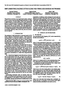
Figure 3.1 below visualizes the data in Table 3.1 SNR of Female Speech 8 7

SNR(dB)

6 5

LPC

4

Lattice

3

LSP

2 1 0 5

10

15

16

17

18

19

20

Order

Figure 3.1 Graph of SNR values of Female Speech From Table 3.1 and Figure 3.1, we can see the maximum SNR values of LPC, Lattice, and LSP are almost the same but the orders (number of coefficients) at which the max values take place are different. LPC achieves max SNR value at the order of 18 while Lattice’s is at the order of 17 and LSP achieves its max SNR at the order of 15 or 16. Similarly, we have SNR values for male speech. Note that the SNR values of male speech are a little less than that of female speech. As we can see in Figure 3.1, Figure 3.2, and Figure 3.3, the SNR values of LPC, Lattice, and LSP start going down after they reach their max values. The reason is that the size of SRAM is only 256 KB so it could not hold both program and data. We should also note the access speed of SRAM is much higher than that of SDRAM. Hence, there are some noises in the gap among voice segments, which in turn decreasing the SNR values. In this implementation, SRAM is utilized to contain as much data as possible and the remainder is put on SDRAM. Male

14

and bird sounds shown in Table 3.2 and Table 3.3 have the same results due to the limit of hardware resources. Table 3.2 SNR Values of Male Speech Order

5

10

15

16

17

18

19

20

LPC

5.0

5.9

6.3

6.4

6.5

6.5

6.3

6.2

Lattice

5.2

6.1

6.4

6.5

6.6

6.4

6.2

6.0

LSP

5.3

6.2

6.4

6.6

6.5

6.3

6.2

5.8

Figure 3.2 below visualizes the data in Table 3.2

SNR of Male Speech 7 6

SNR(dB)

5 LPC

4

Lattice 3

LSP

2 1 0 5

10

15

16

17

18

19

20

Order

Figure 3.2 Graph of SNR values of Male Speech

This project also evaluates the SNR values for bird sounds. The result is shown in Table 3.3 below.

15

Table 3.3 SNR Values of Bird Sounds Order

5

10

15

16

17

18

19

20

LPC

5.3

5.9

6.2

6.3

6.4

6.3

6.2

5.9

Lattice

5.3

6.1

6.3

6.4

6.5

6.4

6.1

5.7

LSP

5.4

6.2

6.4

6.4

6.3

6.0

5.8

5.4

Figure 3.3 below visualizes the data in Table 3.3

SNR of Bird Sounds 7 6

SNR(dB)

5 LPC

4

Lattice 3

LSP

2 1 0 5

10

15

16

17

18

19

20

Order

Figure 3.3 Graph of SNR values of Bird Sounds

3.2 Efficiency Evaluation The performance is evaluated based on four factors: •

The code size of three implementations

•

The memory size of three implementations 16

•

The energy used to code and decode sound signals

•

The delay time or how much time needed to completely analyze the sound input.

Table 3.4 below shows the evaluations of the efficiency of three algorithms: LPC, Lattice, and LSP in five criteria: the size of the source code in nesC language “Code Size 1”, the size of the source code after deploying into imote2 flash memory “Code Size 2”, the size of the program on RAM “Memory Size”, the average power usage to analyze and synthesize sound recordings “Energy”, and the time to analyze and synthesize the recording sounds “Delay Time”.

Table 3.4 Efficiency Evaluation Code Size 1

Code Size 2

Memory Size

Energy

Delay Time

(KB)

(KB)

(KB)

(mW)

(sec)

LPC

4.5

467

370

34

1.1

Lattice

3.2

409

339

37

1.2

LSP

6.7

568

425

45

1.5

Figure 3.4 and Figure 3.5 below visualize the data in Table 3.4

17

Code and Memory Size 600 500

KB

400

LPC

300

Lattice

200

LSP

100 0 (KB)

(KB)

(KB)

Code Size 1

Code Size 2

Memory Size

Size

Figure 3.4 Graph of Code and Memory Size

Power Usage and Delay Time 50 45 40 35 30

LPC

25 20 15 10 5 0

Lattice LSP

(mW)

(sec)

Energy

Delay Time

Figure 3.5 Graph of Power Usage and Delay Time

The statistics above are the total of both analysis and synthesis phases. The statistics for energy and time delay is measured for 10 coefficients. The energy usage and

18

delay time will be greater for higher order analysis-synthesis filter. Note that the memory size for all three algorithms is greater than 256 KB, the size of SRAM of Imote2. It means we have to use SDRAM to run the algorithms that draws much more power than if we only run on SRAM.

3.3 Subjective Testing In this section, the Mean Opinion Score (MOS) is used to evaluate resynthesized sounds [8]. A group of five people is asked to rate the quality of synthesized sounds based on a scale of 1 to 5 (1 = Bad, 2 Poor, 3 = Fair, 4 = Good, 5 = Excellent). Table 3.5 below shows the MOS values of LPC, Lattice, and LSP for female, male, and bird sound recordings. The scores are evaluated by five volunteers who allowed using their voice recordings in this project.

Table 3.5 MOS Values Female

Male

Bird

LPC

3

2

3

Lattice

3

2

3

LSP

4

3

3

Figure 3.6 below visualizes the data in Table 3.5

19

Mean Opinion Score 4.5 4 3.5 Score

3

LPC

2.5

Lattice

2

LSP

1.5 1 0.5 0 Female

Male

Bird

Types of Sounds

Figure 3.6 Graph of Mean Opinion Score

From Table 3.1, Table 3.2, Table 3.3, and Table 3.5, we can see that there are differences between testing based on SNR values and subjective testing. Specifically, although the SNR values of Lattice are greater than that of LPC, the MOS scores of both algorithms are the same. For bird sounds, the MOS scores of three algorithms are the same regardless the differences in SNR values.

20

4. FUTURE WORKS AND CONCLUSIONS This section discusses what this work has achieved and what should be done to improve in the future.

4.1 Future Works Reducing the code size to less than 256 KB can make the program fit in the SRAM, hence, improve the power usage and delay time since SRAM runs faster and does not need to be refreshed. The sound quality can also be improved by using different kind of filters before actually using LPC, Lattice, or LSP filters. Some typical filters can be used are low-pass and high-pass filters. This may add some delay to processing but it can significantly improve the quality of synthesized sounds. A real application to monitor environment will be developed to evaluate the reliability and practicality of the three implementations in this project.

4.2 Conclusions This project describes the new emerging research direction that combines wireless sensor networks and sound processing [6]. In this project, three LPC-based implementations (original LPC, lattice LPC, and LSP) are coded on Crossbow Imote2 platform. To measure the applicability of this program, we evaluate both its efficiency and quality of synthesized sounds. The quality of synthesized sounds is tested using signal-to-noise ratio and mean opinion score while efficiency is measured in terms of code size, memory size, power usage, and processing time. The experimental results show that it is highly practical to process different kinds of sounds using tiny sensor

21

devices. The experiment with bird sounds also shows many potential applications for environmental monitoring using wireless sensor networks.

22

BIBLIOGRPHY AND REFERENCES

[1] Akyildiz, I., Su, W., Sankarasubramaniam, Y., and Cayirci, E., “A survey on sensor networks,” IEEE Communications Magazine, 40(8), pp. 102-114, 2002, Aug. 2002.

[2] Barrenetxea, G., Ingelrest, F., Schaefer, G., and Vetterli, M., “Wireless Sensor Networks for Environmental Monitoring: The SensorScope Experience,” 2008 IEEE International Zurich Seminar on Communications, Zurich, pp. 98-101, Mar. 2008. [3] Cardell-Oliver, R., Smettern, K., Kranz, M., and Mayer, K., “Field Testing a Wireless Sensor Network for Reactive Environmental Monitoring,” Intl. Conference on Intelligent Sensors, Sensor Networks and Information Processing, Dec. 14-17, 2004. [4] Cook, P. R., Real Sound Synthesis for Interactive Applications, A K Peters, 2002. [5] Chu, W. C., Speech Coding Algorithms: Foundation and Evolution of Standardized Coders, Wiley-Interscience, 2003. [6] Ganju, D. and Schwiebert, L., “Using Sound for Monitoring Wireless Sensor Network Behavior,” 2007 ACM/IFIP/USENIX International Conference on Middleware, no. 5, 2007. [7] Hu, W., Tran, V. N., Bulusu, N., Chou, C., Jha, S., Taylor, A.,“The Design and Evaluation of a Hybrid Sensor Network For Cane-toad Monitoring,” Information Processing in Sensor Networks, pp. 25-27, Apr. 2005. [8] Huang, X., Acero, A., and Hon, H. W., Spoken Language Processing: A Guide to Theory, Algorithm, and System Development, Prentice Hall, 2001. [9] Lan, S., Qilong, M., and Du, J., “Architecture of Wireless Sensor Networks for Environmental Monitoring,” International Workshop on Education Technology and Training, 2008. And 2008 International Workshop on Geosciences and Remote Sensing. ETT and GRS 2008, Shanghai, pp. 579-582, Dec. 2008. [10] Mainwaring, A., Culler, D., Polastre, J., Szewczyk, R., and Anderson, J., “Wireless sensor networks for habitat monitoring,” Proceedings of the 1st ACM international workshop on Wireless sensor networks and applications, pp. 88-97, Sept. 28, 2002. [11] Park, S. W., Gomez, M., and Khastri, R., “Speech compression using line spectrum pair frequencies and wavelet transform,” Proc. Intelligent Multimedia, Video and Speech processing, pp. 437-440, 2001. [12] The Freesound Project. http://www.freesound.org/. [13] Tremain, T., "The government standard linear predictive coding algorithm: LPC 10," Speech Technology, 1982, pp. 40 - 49. 23

[14] Vallabha, G. and Tuller, B., “Choice of Filter Order in LPC Analysis of Vowels,” From Sound to Sense, MIT, 2004, pp. C-203 – C-208. [15] XBow Imote2 Data Sheet. http://www.xbow.com/Products/Product_pdf_files/ Wireless_pdf/Imote2_Datasheet.pdf. Retrieved on April 15, 2010.

24

APPENDIX A – WAVEFORM AND SPECTROGRAM This section shows some waveform and spectrum pictures of original and synthesized sounds. They are generated using Matlab and Audacity software.

(a) Waveform of the original speech

(b) Waveform of the synthesized speech Figure 1. Time waveform of a female voice saying “digital signal processing”.

25

(a) Spectrogram of the original speech

(b) Spectrogram of the synthesized speech Figure 2. Spectrogram of a female voice saying “digital signal processing”.

26

APPENDIX B – SOURCE CODE This section shows main functions of the program. File LPC.nc: configuration LPC { } implementation { components Main, WM8940C, LPCM, RandomLFSR; Main.StdControl -> LPCM; LPCM.CodecControl -> WM8940C.StdControl; LPCM.Audio -> WM8940C.Audio; LPCM.Random -> RandomLFSR; }

File LPCM.nc: module LPCM{ provides{ interface StdControl; } uses{ interface Audio; interface StdControl as CodecControl; interface Random; } } implementation{ #define numCoef 10 #define BLOCK_SIZE 240 //8KHz*30ms #define HOP_SIZE 160 //8KHz*20ms #define ORDER 10 #define SDRAM_BUFFER_SIZE 48768 #define SRAM_BUFFER_SIZE 32768 #define PROC_DATA_SIZE ((SDRAM_BUFFER_SIZE+SRAM_BUFFER_SIZE)/2) #define NUM_BLK (((SDRAM_BUFFER_SIZE/4) + (SRAM_BUFFER_SIZE/4))/HOP_SIZE + 1) uint32_t gSDBuffer[SDRAM_BUFFER_SIZE] __attribute__((section(".sdram"),aligned(32))); uint32_t gSDNumSamples = SDRAM_BUFFER_SIZE/4; uint32_t gSBuffer[SRAM_BUFFER_SIZE] __attribute__((aligned(32))); uint32_t gSNumSamples = SRAM_BUFFER_SIZE/4; float gData[PROC_DATA_SIZE] __attribute__((section(".sdram"))); uint32_t gCount = 0, gNumSamples = 0; command result_t StdControl.init(){ result_t res;

27

//perform custom initialization here call Random.init(); res = call CodecControl.init(); return res; } command result_t StdControl.start(){ result_t res; //perform custom starting here res = call CodecControl.start(); return res; } command result_t StdControl.stop(){ //perform custom stopping here result_t res; res = call CodecControl.stop(); return res; } void preProcessing() { uint32_t i; //copy & convert data from stereo to mono on the fly //Can be improved by recording mono channel at the beginning for anyone who wants to improve the performance of this program for( i=0; i