LOGISTIC REGRESSION: BINARY AND MULTINOMIAL

2014 Edition

Copyright @c 2014 by G. David Garson and Statistical Associates Publishing

Page 1

LOGISTIC REGRESSION: BINARY AND MULTINOMIAL

2014 Edition

@c 2014 by G. David Garson and Statistical Associates Publishing. All rights reserved worldwide in all media.

ISBN: 978-1-62638-024-0 The author and publisher of this eBook and accompanying materials make no representation or warranties with respect to the accuracy, applicability, fitness, or completeness of the contents of this eBook or accompanying materials. The author and publisher disclaim any warranties (express or implied), merchantability, or fitness for any particular purpose. The author and publisher shall in no event be held liable to any party for any direct, indirect, punitive, special, incidental or other consequential damages arising directly or indirectly from any use of this material, which is provided “as is”, and without warranties. Further, the author and publisher do not warrant the performance, effectiveness or applicability of any sites listed or linked to in this eBook or accompanying materials. All links are for information purposes only and are not warranted for content, accuracy or any other implied or explicit purpose. This eBook and accompanying materials is © copyrighted by G. David Garson and Statistical Associates Publishing. No part of this may be copied, or changed in any format, sold, rented, or used commercially in any way under any circumstances. Contact: G. David Garson, President Statistical Publishing Associates 274 Glenn Drive Asheboro, NC 27205 USA Email: [email protected] Web: www.statisticalassociates.com

Copyright @c 2014 by G. David Garson and Statistical Associates Publishing

Page 2

LOGISTIC REGRESSION: BINARY AND MULTINOMIAL

2014 Edition

Table of Contents Page numbering words in the full edition. This is the preview edition of the first 25 pages.

Overview ....................................................................................................................................... 10 Data examples............................................................................................................................... 12 Key Terms and Concepts............................................................................................................... 13 Binary, binomial, and multinomial logistic regression .............................................................. 13 The logistic model ..................................................................................................................... 14 The logistic equation ............................................................................................................. 15 Logits and link functions ........................................................................................................ 17 Saving predicted probabilities ............................................................................................... 19 The dependent variable ............................................................................................................ 20 The dependent reference default in binary logistic regression ............................................ 21 The dependent reference default in multinomial logistic regression ................................... 22 Factors: Declaring ......................................................................... Error! Bookmark not defined. Overview ................................................................................... Error! Bookmark not defined. SPSS........................................................................................... Error! Bookmark not defined. SAS ............................................................................................ Error! Bookmark not defined. Stata .......................................................................................... Error! Bookmark not defined. Factors: Reference levels ............................................................. Error! Bookmark not defined. Overview ................................................................................... Error! Bookmark not defined. SPSS........................................................................................... Error! Bookmark not defined. SAS ............................................................................................ Error! Bookmark not defined. Stata .......................................................................................... Error! Bookmark not defined. Covariates ..................................................................................... Error! Bookmark not defined. Overview ................................................................................... Error! Bookmark not defined. SPSS........................................................................................... Error! Bookmark not defined. SAS ............................................................................................ Error! Bookmark not defined. Stata .......................................................................................... Error! Bookmark not defined. Interaction Terms ......................................................................... Error! Bookmark not defined. Overview ................................................................................... Error! Bookmark not defined. SPSS........................................................................................... Error! Bookmark not defined. SAS ............................................................................................ Error! Bookmark not defined. Stata .......................................................................................... Error! Bookmark not defined. Estimation .................................................................................... Error! Bookmark not defined. Overview ................................................................................... Error! Bookmark not defined. Maximum likelihood estimation (ML) ...................................... Error! Bookmark not defined. Weighted least squares estimation (WLS) ............................... Error! Bookmark not defined. Ordinary least squares estimation (OLS) .................................. Error! Bookmark not defined. A basic binary logistic regression model in SPSS ............................. Error! Bookmark not defined. Copyright @c 2014 by G. David Garson and Statistical Associates Publishing

Page 3

LOGISTIC REGRESSION: BINARY AND MULTINOMIAL

2014 Edition

Example ........................................................................................ Error! Bookmark not defined. SPSS input ..................................................................................... Error! Bookmark not defined. SPSS output .................................................................................. Error! Bookmark not defined. Parameter estimates and odds ratios ...................................... Error! Bookmark not defined. Omnibus tests of model coefficients ........................................ Error! Bookmark not defined. Model summary........................................................................ Error! Bookmark not defined. Classification table .................................................................... Error! Bookmark not defined. Classification plot...................................................................... Error! Bookmark not defined. Hosmer-Lemeshow test of goodness of fit .............................. Error! Bookmark not defined. Casewise listing of residuals for outliers > 2 standard deviationsError! Bookmark not defined. A basic binary logistic regression model in SAS ............................... Error! Bookmark not defined. Example ........................................................................................ Error! Bookmark not defined. SAS input ...................................................................................... Error! Bookmark not defined. Reconciling SAS and SPSS output ............................................. Error! Bookmark not defined. SAS output .................................................................................... Error! Bookmark not defined. Parameter estimates ................................................................ Error! Bookmark not defined. Odds ratio estimates ................................................................ Error! Bookmark not defined. Global null hypothesis tests...................................................... Error! Bookmark not defined. Model fit statistics .................................................................... Error! Bookmark not defined. The classification table ............................................................. Error! Bookmark not defined. The association of predicted probabilities and observed responses tableError! Bookmark not defined. Hosmer and Lemeshow test of goodness of fit ........................ Error! Bookmark not defined. Regression diagnostics table .................................................... Error! Bookmark not defined. A basic binary logistic regression model in STATA .......................... Error! Bookmark not defined. Overview and example................................................................. Error! Bookmark not defined. Data setup .................................................................................... Error! Bookmark not defined. Stata input .................................................................................... Error! Bookmark not defined. Stata output ................................................................................. Error! Bookmark not defined. Parameter estimates ................................................................ Error! Bookmark not defined. Odds ratios................................................................................ Error! Bookmark not defined. Likelihood ratio test of the model ............................................ Error! Bookmark not defined. Model fit statistics .................................................................... Error! Bookmark not defined. The classification table ............................................................. Error! Bookmark not defined. Classification plot...................................................................... Error! Bookmark not defined. Measures of association ........................................................... Error! Bookmark not defined. Hosmer-Lemeshow test............................................................ Error! Bookmark not defined. Residuals and regression diagnostics ....................................... Error! Bookmark not defined. A basic multinomial logistic regression model in SPSS .................... Error! Bookmark not defined. Example ........................................................................................ Error! Bookmark not defined. Model ........................................................................................... Error! Bookmark not defined. SPSS statistical output .................................................................. Error! Bookmark not defined. Copyright @c 2014 by G. David Garson and Statistical Associates Publishing

Page 4

LOGISTIC REGRESSION: BINARY AND MULTINOMIAL

2014 Edition

Step summary ........................................................................... Error! Bookmark not defined. Model fitting information table................................................ Error! Bookmark not defined. Goodness of fit tests ................................................................. Error! Bookmark not defined. Likelihood ratio tests ................................................................ Error! Bookmark not defined. Parameter estimates ................................................................ Error! Bookmark not defined. Pseudo R-square ....................................................................... Error! Bookmark not defined. Classification table .................................................................... Error! Bookmark not defined. Observed and expected frequencies ........................................ Error! Bookmark not defined. Asymptotic correlation matrix.................................................. Error! Bookmark not defined. A basic multinomial logistic regression model in SAS ..................... Error! Bookmark not defined. Example ........................................................................................ Error! Bookmark not defined. SAS syntax .................................................................................... Error! Bookmark not defined. SAS statistical output.................................................................... Error! Bookmark not defined. Overview ................................................................................... Error! Bookmark not defined. Model fit ................................................................................... Error! Bookmark not defined. Goodness of fit tests ................................................................. Error! Bookmark not defined. Parameter estimates ................................................................ Error! Bookmark not defined. Pseudo R-Square....................................................................... Error! Bookmark not defined. Classification table .................................................................... Error! Bookmark not defined. Observed and predicted functions and residuals..................... Error! Bookmark not defined. Correlation matrix of estimates................................................ Error! Bookmark not defined. A basic multinomial logistic regression model in STATA ................. Error! Bookmark not defined. Example ........................................................................................ Error! Bookmark not defined. Stata data setup ........................................................................... Error! Bookmark not defined. Stata syntax .................................................................................. Error! Bookmark not defined. Stata statistical output ................................................................. Error! Bookmark not defined. Overview ................................................................................... Error! Bookmark not defined. Model fit ................................................................................... Error! Bookmark not defined. AIC and BIC ............................................................................... Error! Bookmark not defined. Pseudo R-square ....................................................................... Error! Bookmark not defined. Goodness of fit test .................................................................. Error! Bookmark not defined. Likelihood ratio tests ................................................................ Error! Bookmark not defined. Parameter estimates ................................................................ Error! Bookmark not defined. Odds ratios/ relative risk ratios ................................................ Error! Bookmark not defined. Classification table .................................................................... Error! Bookmark not defined. Observed and expected frequencies ........................................ Error! Bookmark not defined. Asymptotic correlation matrix.................................................. Error! Bookmark not defined. ROC curve analysis ........................................................................... Error! Bookmark not defined. Overview ...................................................................................... Error! Bookmark not defined. Comparing models.................................................................... Error! Bookmark not defined. Optimal classification cutting points ........................................ Error! Bookmark not defined. Example ........................................................................................ Error! Bookmark not defined. SPSS .............................................................................................. Error! Bookmark not defined. Copyright @c 2014 by G. David Garson and Statistical Associates Publishing

Page 5

LOGISTIC REGRESSION: BINARY AND MULTINOMIAL

2014 Edition

Comparing models.................................................................... Error! Bookmark not defined. Optimal classification cutting points ........................................ Error! Bookmark not defined. SAS ................................................................................................ Error! Bookmark not defined. Overview ................................................................................... Error! Bookmark not defined. Comparing Models ................................................................... Error! Bookmark not defined. Optimal classification cutting points ........................................ Error! Bookmark not defined. Stata ............................................................................................. Error! Bookmark not defined. Overview ................................................................................... Error! Bookmark not defined. Comparing Models ................................................................... Error! Bookmark not defined. Optimal classification cutting points ........................................ Error! Bookmark not defined. Conditional logistic regression for matched pairs ........................... Error! Bookmark not defined. Overview ...................................................................................... Error! Bookmark not defined. Example ........................................................................................ Error! Bookmark not defined. Data setup .................................................................................... Error! Bookmark not defined. Conditional logistic regression in SPSS ......................................... Error! Bookmark not defined. Overview ................................................................................... Error! Bookmark not defined. SPSS input ................................................................................. Error! Bookmark not defined. SPSS output............................................................................... Error! Bookmark not defined. Conditional logistic regression in SAS .......................................... Error! Bookmark not defined. Overview ................................................................................... Error! Bookmark not defined. SAS input ................................................................................... Error! Bookmark not defined. SAS output ................................................................................ Error! Bookmark not defined. Conditional logistic regression in Stata ........................................ Error! Bookmark not defined. Overview ................................................................................... Error! Bookmark not defined. Stata input ................................................................................ Error! Bookmark not defined. Stata output .............................................................................. Error! Bookmark not defined. More about parameter estimates and odds ratios ......................... Error! Bookmark not defined. For binary logistic regression ....................................................... Error! Bookmark not defined. Example 1 ................................................................................. Error! Bookmark not defined. Example 2 ................................................................................. Error! Bookmark not defined. For multinomial logistic regression .............................................. Error! Bookmark not defined. Example 1 ................................................................................. Error! Bookmark not defined. Example 2 ................................................................................. Error! Bookmark not defined. Coefficient significance and correlation significance may differ . Error! Bookmark not defined. Reporting odds ratios ................................................................... Error! Bookmark not defined. Odds ratios: Summary .................................................................. Error! Bookmark not defined. Effect size ..................................................................................... Error! Bookmark not defined. Confidence interval on the odds ratio ...................................... Error! Bookmark not defined. Warning: very high or very low odds ratios ............................. Error! Bookmark not defined. Comparing the change in odds for different values of X.......... Error! Bookmark not defined. Comparing the change in odds when interaction terms are in the modelError! Bookmark not defined. Probabilities, logits, and odds ratios ............................................ Error! Bookmark not defined. Copyright @c 2014 by G. David Garson and Statistical Associates Publishing

Page 6

LOGISTIC REGRESSION: BINARY AND MULTINOMIAL

2014 Edition

Probabilities .............................................................................. Error! Bookmark not defined. Relative risk ratios (RRR)........................................................... Error! Bookmark not defined. More about significance tests.......................................................... Error! Bookmark not defined. Overview ...................................................................................... Error! Bookmark not defined. Significance of the model ............................................................. Error! Bookmark not defined. SPSS........................................................................................... Error! Bookmark not defined. SAS ............................................................................................ Error! Bookmark not defined. Stata .......................................................................................... Error! Bookmark not defined. Significance of parameter effects ................................................ Error! Bookmark not defined. SPSS........................................................................................... Error! Bookmark not defined. SAS ............................................................................................ Error! Bookmark not defined. Stata .......................................................................................... Error! Bookmark not defined. More about effect size measures .................................................... Error! Bookmark not defined. Overview ...................................................................................... Error! Bookmark not defined. Effect size for the model .............................................................. Error! Bookmark not defined. Pseudo R-squared ..................................................................... Error! Bookmark not defined. Classification tables .................................................................. Error! Bookmark not defined. Terms associated with classification tables: ............................ Error! Bookmark not defined. The c statistic ............................................................................ Error! Bookmark not defined. Information theory measures of model fit ............................... Error! Bookmark not defined. Effect size for parameters ............................................................ Error! Bookmark not defined. Odds ratios................................................................................ Error! Bookmark not defined. Standardized vs. unstandardized logistic coefficients in model comparisons ................. Error! Bookmark not defined. Stepwise logistic regression ......................................................... Error! Bookmark not defined. Overview ................................................................................... Error! Bookmark not defined. Forward selection vs. backward elimination ............................ Error! Bookmark not defined. Cross-validation ........................................................................ Error! Bookmark not defined. Rao's efficient score as a variable entry criterion for forward selectionError! Bookmark not defined. Score statistic............................................................................ Error! Bookmark not defined. Which step is the best model? ................................................. Error! Bookmark not defined. Contrast Analysis .......................................................................... Error! Bookmark not defined. Repeated contrasts................................................................... Error! Bookmark not defined. Indicator contrasts.................................................................... Error! Bookmark not defined. Contrasts and ordinality ........................................................... Error! Bookmark not defined. Analysis of residuals ......................................................................... Error! Bookmark not defined. Overview ...................................................................................... Error! Bookmark not defined. Residual analysis in binary logistic regression ............................. Error! Bookmark not defined. Outliers ..................................................................................... Error! Bookmark not defined. The DfBeta statistic................................................................... Error! Bookmark not defined. The leverage statistic ................................................................ Error! Bookmark not defined. Cook's distance ......................................................................... Error! Bookmark not defined. Copyright @c 2014 by G. David Garson and Statistical Associates Publishing

Page 7

LOGISTIC REGRESSION: BINARY AND MULTINOMIAL

2014 Edition

Residual analysis in multinomial logistic regression .................... Error! Bookmark not defined. Assumptions..................................................................................... Error! Bookmark not defined. Data level ...................................................................................... Error! Bookmark not defined. Meaningful coding........................................................................ Error! Bookmark not defined. Proper specification of the model................................................ Error! Bookmark not defined. Independence of irrelevant alternatives...................................... Error! Bookmark not defined. Error terms are assumed to be independent (independent sampling)Error! Bookmark not defined. Low error in the explanatory variables ........................................ Error! Bookmark not defined. Linearity ........................................................................................ Error! Bookmark not defined. Additivity ...................................................................................... Error! Bookmark not defined. Absence of perfect separation ..................................................... Error! Bookmark not defined. Absence of perfect multicollinearity ............................................ Error! Bookmark not defined. Absence of high multicollinearity................................................. Error! Bookmark not defined. Centered variables ....................................................................... Error! Bookmark not defined. No outliers .................................................................................... Error! Bookmark not defined. Sample size ................................................................................... Error! Bookmark not defined. Sampling adequacy ...................................................................... Error! Bookmark not defined. Expected dispersion ..................................................................... Error! Bookmark not defined. Frequently Asked Questions ............................................................ Error! Bookmark not defined. How should logistic regression results be reported?................... Error! Bookmark not defined. Example .................................................................................... Error! Bookmark not defined. Why not just use regression with dichotomous dependents? .... Error! Bookmark not defined. How does OLS regression compare to logistic regression? ......... Error! Bookmark not defined. When is discriminant analysis preferred over logistic regression?Error! Bookmark not defined. What is the SPSS syntax for logistic regression? .......................... Error! Bookmark not defined. Apart from indicator coding, what are the other types of contrasts?Error! Bookmark not defined. Can I create interaction terms in my logistic model, as with OLS regression?Error! Bookmark not defined. Will SPSS's binary logistic regression procedure handle my categorical variables automatically? .............................................................................. Error! Bookmark not defined. Can I handle missing cases the same in logistic regression as in OLS regression? .............. Error! Bookmark not defined. Explain the error message I am getting about unexpected singularities in the Hessian matrix. ...................................................................................................... Error! Bookmark not defined. Explain the error message I am getting in SPSS about cells with zero frequencies. ........... Error! Bookmark not defined. Is it true for logistic regression, as it is for OLS regression, that the beta weight (standardized logit coefficient) for a given independent reflects its explanatory power controlling for other variables in the equation, and that the betas will change if variables are added or dropped from the equation? ...................................................................... Error! Bookmark not defined. Copyright @c 2014 by G. David Garson and Statistical Associates Publishing

Page 8

LOGISTIC REGRESSION: BINARY AND MULTINOMIAL

2014 Edition

What is the coefficient in logistic regression which corresponds to R-Square in multiple regression? ................................................................................... Error! Bookmark not defined. Is multicollinearity a problem for logistic regression the way it is for multiple linear regression? ................................................................................... Error! Bookmark not defined. What is the logistic equivalent to the VIF test for multicollinearity in OLS regression? Can odds ratios be used? .................................................................... Error! Bookmark not defined. How can one use estimated variance of residuals to test for model misspecification? ..... Error! Bookmark not defined. How are interaction effects handled in logistic regression?........ Error! Bookmark not defined. Does stepwise logistic regression exist, as it does for OLS regression?Error! Bookmark not defined. What are the stepwise options in multinomial logistic regression in SPSS?Error! Bookmark not defined. May I use the multinomial logistic option when my dependent variable is binary? ........... Error! Bookmark not defined. What is nonparametric logistic regression and how is it more nonlinear?Error! Bookmark not defined. How many independent variables can I have? ............................ Error! Bookmark not defined. How do I express the logistic regression equation if one or more of my independent variables is categorical? ............................................................................... Error! Bookmark not defined. How do I compare logit coefficients across groups formed by a categorical independent variable? ....................................................................................... Error! Bookmark not defined. How do I compute the confidence interval for the unstandardized logit (effect) coefficients? ...................................................................................................... Error! Bookmark not defined. Acknowledgments............................................................................ Error! Bookmark not defined. Bibliography ..................................................................................... Error! Bookmark not defined.

Copyright @c 2014 by G. David Garson and Statistical Associates Publishing

Page 9

LOGISTIC REGRESSION: BINARY AND MULTINOMIAL

2014 Edition

Overview Binary logistic regression is a form of regression which is used when the dependent variable is a true or forced dichotomy and the independent variables are of any type. Multinomial logistic regression exists to handle the case of dependent variables with more classes than two, though it is sometimes used for binary dependent variables as well since it generates somewhat different output, described below. Logistic regression can be used to predict a categorical dependent variable on the basis of continuous and/or categorical independent variables; to determine the effect size of the independent variables on the dependent variable; to rank the relative importance of independent variables; to assess interaction effects; and to understand the impact of covariate control variables. The impact of predictor variables is usually explained in terms of odds ratios, which is the key effect size measure for logistic regression. Logistic regression applies maximum likelihood estimation after transforming the dependent into a logit variable. A logit is the natural log of the odds of the dependent equaling a certain value or not (usually 1 in binary logistic models, or the highest value in multinomial models). Logistic regression estimates the odds of a certain event (value) occurring. This means that logistic regression calculates changes in the log odds of the dependent, not changes in the dependent itself as does OLS regression. Logistic regression has many analogies to OLS regression: logit coefficients correspond to b coefficients in the logistic regression equation; the standardized logit coefficients correspond to beta weights; and a pseudo R2 statistic is available to summarize the overall strength of the model. Unlike OLS regression, however, logistic regression does not assume linearity of relationship between the raw values of the independent variables and raw values of the dependent; does not require normally distributed variables; does not assume homoscedasticity; and in general has less stringent requirements. Logistic regression does, however, require that observations be independent and that the independent variables be linearly related to the logit of the dependent. The predictive success of logistic regression can be assessed by looking at the classification table, showing correct and incorrect classifications of the Copyright @c 2014 by G. David Garson and Statistical Associates Publishing

Page 10

LOGISTIC REGRESSION: BINARY AND MULTINOMIAL

2014 Edition

dichotomous, ordinal, or polytomous dependent variable. Goodness-of-fit tests such as the likelihood ratio test are available as indicators of model appropriateness, as is the Wald statistic to test the significance of individual independent variables. Procedures related to logistic regression but not treated in the current volume include generalized linear models, ordinal regression, log-linear analysis, and logit regression, briefly described below. Binary and multinomial logistic regression may be implemented in stand-alone statistical modules described in this volume or in statistical modules for generalized linear modeling (GZLM), available in most statistical packages. GZLM provides allows the researcher to create regression models with any distribution of the dependent (ex., binary, multinomial, ordinal) and any link function (ex., log for logilinear analysis, logit for binary or multinomial logistic analysis, cumulative logit for ordinal logistic analysis, and many others). Similarly, generalized linear mixed modeling (GLMM) is now available to handle multilevel logistic modeling. These topics are also treated separately in their own volumes in the Statistical Associates 'Blue Book' series. When multiple classes of a multinomial dependent variable can be ranked by order, then ordinal logistic regression is preferred to multinomial logistic regression since ordinal regression has higher power for ordinal data. (Ordinal regression is discussed in the separate Statistical Associates’ "Blue Book" volume, Ordinal Regression.) Also, logistic regression is not used when the dependent variable is continuous, nor when there is more than one dependent variable (compare logit regression, which allows multiple dependent variables). Note that in its “Complex Samples” add-on module, SPSS supports “complex samples logistic regression” (CSLOGISTIC). This module is outside the scope of this volume but operates in a largely similar manner to support data drawn from complex samples and has a few capabilities not found in its ordinary LOGISTIC procedure (ex., nested terms). Likewise, all packages described in this volume have additional options and capabilities not covered in this volume, which is intended as an introductory rather than comprehensive graduate-level discussion of logistic regression.

Copyright @c 2014 by G. David Garson and Statistical Associates Publishing

Page 11

LOGISTIC REGRESSION: BINARY AND MULTINOMIAL

2014 Edition

Logit regression, treated in the Statistical Associates 'Blue Book' volume, Loglinear Analysis, is another option related to logistic regression. For problems with one dependent variable and where both are applicable, logit regression has numerically equivalent results to logistic regression, but with different output options. For the same class of problems, logistic regression has become more popular among social scientists. Loglinear analysis applies logistic methods to the analysis of categorical data, typically crosstabulations.

Data examples The example datasets used in this volume are listed below in order of use, with versions for SPSS (.sav), SAS (.sas7bdat), and Stata (.dta). The sections on binary and multinomial regression use survey data in a file called “GSS93subset”. Variables are described below. • Click here to download GSS93subset.sav for SPSS. • Click here to download GSS93subset.sas7bdat for SAS. • Click here to download GSS93subset.dta for Stata. The section on ROC curves uses data in a file called “auto”, dealing with characteristics of 1978 automobiles. It is supplied as a sample data file with Stata. • Click here to download auto.sav for SPSS. • Click here to download auto.sas7bdat for SAS. • Click here to download auto.dta for Stata. The section on conditional matched pairs logistic regression uses data in a file called “BreslowDaySubset”, dealing with causes of endometrial cancer. See Breslow & Day (1980). • Click here to download BreslowDaySubset.sav for SPSS. • Click here to download BreslowDaySubset2.sav for SPSS. This contains differenced data required by the SPSS approach, as discussed in the SPSS conditional logistic regression section. • Click here to download BreslowDaySubset.sas7bdat for SAS. • Click here to download BreslowDaySubset.dta for Stata.

Copyright @c 2014 by G. David Garson and Statistical Associates Publishing

Page 12

LOGISTIC REGRESSION: BINARY AND MULTINOMIAL

2014 Edition

Key Terms and Concepts Binary, binomial, and multinomial logistic regression Though the terms "binary" and "binomial" are often used interchangeably, they are not. Binary logistic regression, discussed in this volume, deals with dependent variables which have two values, usually coded 0 and 1 (ex., for sex, 0 = male and 1 = female). These two values may represent a true dichotomy, as for gender, or may represent a forced dichotomy, such as high and low income. In contrast, binomial logistic regression is used where the dependent variable is not a binary variable per se, but rather is a count based on a binary variable. To take a classic binomial example, subjects may be told to flip a coin 100 times, with each subject tallying the number of "heads", with the tally being the dependent variable in binomial logistic regression. More realistically, the dependent variable is apt to be a tally of successes (ex., spotting a signal amid visual noise in a psychology experiment). Binomial logistic regression is implemented in generalized linear modeling of count variables, as discussed in the separate Statistical Associates 'Blue Book' volume on “Generalized Linear Models”. For instance, to implement binomial regression in SPSS, under the menu selection Analyze > Generalized Linear Models > Generalized Linear Models, select “Binary logistic” under the Type of Model" tab, then under the Response tab, enter a binomial count variable (ex., "successes") as the dependent variable and also select the "Number of events occurring in a set of trials" radio button to enter the number of trials (ex.,, 100) or if number of trials varies by subject, the name of the number-of-trials variable. Multinomial logistic regression extends binary logistic regression to cover categorical dependent variables with two or more levels. Multinomial logistic regression does not assume the categories are ordered (ordinal regression, another variant in the logistic procedures family, is used if they are, as discussed above). Though typically used where the dependent variable has three classes or more, researchers may use it even with binary dependent variables because output tables differ between multinomial and binary logistic regression procedures. To implement binary logistic regression in SPSS, select Analyze > Regression > Binary Logistic. PROC LOGISTIC is used in SAS to implement binary logistic Copyright @c 2014 by G. David Garson and Statistical Associates Publishing

Page 13

LOGISTIC REGRESSION: BINARY AND MULTINOMIAL

2014 Edition

regression, as described below. In STATA, binary logistic regression is implemented with the logistic or logit commands, as described below. To implement multinomial logistic regression in SPSS, select Analyze > Regression > Multinomial Logistic. PROC CATMOD is used in SAS to implement multinomial logistic regression, as described below. In STATA, multinomial logistic regression is implemented with the mlogit command, as described below.

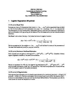
The logistic model The logistic curve, illustrated below, is better for modeling binary dependent variables coded 0 or 1 because it comes closer to hugging the y=0 and y=1 points on the y axis, as illustrated below. Even more, the logistic function is bounded by 0 and 1, whereas the OLS regression function may predict values above 1 and below 0. Logistic analysis can be extended to multinomial dependents by modeling a series of binary comparisons: the lowest value of the dependent compared to a reference category (by default the highest category), the nextlowest value compared to the reference category, and so on, creating k - 1 binary model equations for the k values of the multinomial dependent variable. Ordinal regression also decomposes into a series of binary logistic comparisons.

Copyright @c 2014 by G. David Garson and Statistical Associates Publishing

Page 14

LOGISTIC REGRESSION: BINARY AND MULTINOMIAL

2014 Edition

The logistic equation Logistic regression centers on the following terms: • Odds: An odds is a ratio formed by the probability that an event occurs divided by the probability that the event does not occur. In binary logistic regression, the odds is usually the probability of getting a “1” divided by the probability of getting a “0”. That is, in binary logistic regression, “1” is predicted and “0” is usually the reference category. In multinomial logistic regression, any lower value may be predicted and the highest-coded value is usually the reference category. • Odds ratio: An odds ratio is the ratio of two odds, such as the ratio of the odds for men and the odds for women. Odds ratios are the main effect size measure for logistic regression, reflecting in this case what difference gender makes as a predictor of some dependent variable. An odds ratio of 1.0 (which is 1:1 odds) indicates the variable has no effect. The further from 1.0 in either direction, the greater the effect. • Log odds: The log odds is the coefficient predicted by logistic regression and is called the “logit”. It is the natural log of the odds of the dependent Copyright @c 2014 by G. David Garson and Statistical Associates Publishing

Page 15

LOGISTIC REGRESSION: BINARY AND MULTINOMIAL

2014 Edition

variable equaling some value (ex., 1 rather than 0 in binary logistic regression). The log odds thus equals the natural log of the probability of the event occurring divided by the probability of the event not occurring: ln(odds(event)) = ln(prob(event)/prob(nonevent)) • Logit: The “logit function” is the function used in logistic regression to transform the dependent variable prior to attempting to predict it. Specifically, the logit function in logistic regression is the log odds, explained above. The “logit” is the predicted value of the dependent variable. “Logit coefficients” are the b coefficients in the logistic equation used to arrive at the predicted value. Some texts label these logistic b coefficients as “logits,” but this terminology is not recommended in this volume. • Parameter estimates: These are the logistic (logit or b) regression coefficients for the independent variables and the constant in a logistic regression equation, much like the b coefficients in OLS regression. Synonyms for parameter estimates are unstandardized logistic regression coefficients, logit coefficients, log odds-ratios, and effect coefficients. Parameter estimates are on the right-hand side of the logistic regression equation and logits are on the left-hand side. The logistic regression equation itself is: z = b0 + b1X1 + b2X2 + ..... + bkXk • Where z is the log odds of the dependent variable = ln(odds(event)). The "z" is the “logit”, also called the log odds. • The b0 term is the constant or intercept term in the equation. It reflects the log odds (logit estimate) of the dependent variable when model predictors are evaluated at zero. As often 0 will be outside the range of predictor variables. Intercepts will be more interpretable if predictors are centered around their means prior to analysis because then the intercepts are the log odds of the dependent when predictors are at their mean values. In binary logistic regression, there is one intercept estimate. In multinomial logistic regression, there are (k - 1) intercepts, where k is the number of categories of the dependent variable and 1 is subtracted for the reference value.

Copyright @c 2014 by G. David Garson and Statistical Associates Publishing

Page 16

LOGISTIC REGRESSION: BINARY AND MULTINOMIAL

2014 Edition

• There are k independent (X) variables, some of which may be interaction terms. • The "b" terms are the logistic regression coefficients, also called parameter estimates. Some textbooks call these “logits” but that usage is disparaged in this volume. • Exp(b) = the odds ratio for an independent variable = the natural log base e raised to the power of b. The odds ratio of an independent variable is the factor by which the independent variable increases or (if negative) decreases the log odds of the dependent variable The term “odds ratio” usually refers to odds ratios for independent variables. See further discussion of interpreting b parameters below. To convert the log odds (which is z, which is the logit) back into an odds ratio, the natural logarithmic base e is raised to the zth power: odds(event) = exp(z) = the odds ratio for the dependent variable. Exp(z) is thus the estimate of the odds(event). For binary logistic regression, it usually is the estimate for the odds that the dependent = 1. For multinomial logistic regression, it usually is the estimate for the odds that the dependent equals the a given value rather than the highest-coded value. Put another way, logistic regression predicts the log odds of the dependent event. The "event" is a particular value of y, the dependent variable. By default the event is y = 1 for binary dependent variables coded 0,1, and the reference category is 0. For multinomial values event is y equals the value of interest and the reference category is usually the highest value of y. Note this means that for a binary dependent variable coded (0, 1), the reference category is 0 in binary logistic regression but 1 when run in multinomial logistic regression. That is, multinomial regression flips the reference value from lowest to highest. Beware that what value is predicted and what value is the default reference category in logistic regression may vary by software package and by whether binary or multinomial regression is requested. This is discussed in the section which follows. Logits and link functions Overview

Copyright @c 2014 by G. David Garson and Statistical Associates Publishing

Page 17

LOGISTIC REGRESSION: BINARY AND MULTINOMIAL

2014 Edition

As discussed above, logits are the log odds of the event occurring (usually, that the dependent = 1 rather than 0). Parameter estimates (b coefficients) associated with explanatory variables are estimators of the change in the logit caused by a unit change in the independent. In SPSS output, the parameter estimates appear in the "B" column of the "Variables in the Equation" table. Logits do not appear but must be estimated using the logistic regression equation above, inserting appropriate values for the constant and X variable(s). The b coefficients vary between plus and minus infinity, with 0 indicating the given explanatory variable does not affect the logit (that is, makes no difference in the probability of the dependent value equaling the value of the event, usually 1); positive or negative b coefficients indicate the explanatory variable increases or decreases the logit of the dependent. Exp(b) is the odds ratio for the explanatory variable, discussed below. Link functions Parameter estimates on the right-hand side of the logistic regression formula are related to the logit values being estimated on the left-hand side by way of a link function. (1) OLS regression uses an identity link function, meaning the predicted dependent variable is a direct function of the values of the independent variables. (2) Binary logistic regression uses the logit link to create a logistic model whose distribution hugs the 0 and 1 values of the Y axis for a binary dependent and, moreover, does not extrapolate out of range (below 0 or above 1). (3) Multinomial logistic regression also uses the logit link, setting up a series of binary comparisons between the given level of the dependent and the reference level (by default, the highest coded level). (4) Ordinal logistic regression uses a cumulative logit link, setting up a series of binary comparisons between the given level or lower compared to higher levels. (Technically, the SPSS Analyze, Regression, Ordinal menu choice runs the PLUM procedure, which uses a logit link, but the logit link is used to fit a cumulative logit model. The SPSS Analyze, Generalized Linear Models, Generalized linear Models menu choice for ordinal regression assumes an ordered multinomial distribution with a cumulative logit link). Copyright @c 2014 by G. David Garson and Statistical Associates Publishing

Page 18

LOGISTIC REGRESSION: BINARY AND MULTINOMIAL

2014 Edition

Logit coefficients, and why they are preferred over odds ratios in modeling Note that for the case of decrease the odds ratio can vary only from 0 to .999, while for the case of increase it can vary from just over 1.0 to infinity. This asymmetry is a drawback to using the odds ratio as a measure of strength of relationship. Odds ratios are preferred for interpretation, but logit coefficients are preferred in the actual mathematics of logistic models. The odds ratio is a different way of presenting the same information as the unstandardized logit (effect) coefficient. Odds ratios were defined above and are discussed at greater length in sections below. Saving predicted probabilities Predicted probability values and other coefficients may be saved as additional columns added to the dataset (1) SPSS: Use the "Save" button dialogs of binary and multinomial logistic regression dialogs in SPSS, illustrated below.

(2) SAS: Use the OUTPUT= statement to save predicted values or other coefficients. For instance, the statement below creates a new SAS dataset called “mydata” containing the variables predprob, lowlimit, and highlimit. These are respectively the predicted probability of the case and the lower and upper confidence limits on the predicted probability. OUTPUT OUT=mydata PREDICTED=predprob LOWER=lowlimit UPPER=highlimit ;

Copyright @c 2014 by G. David Garson and Statistical Associates Publishing

Page 19

LOGISTIC REGRESSION: BINARY AND MULTINOMIAL

2014 Edition

(3) Stata: The post-estimation command predict prob, pr adds a variable called “prob” to the dataset, containing predicted probabilities. File > Save or File >Save As saves the dataset.

The dependent variable Binary and multinomial logistic regression support only a single dependent variable. For binary logistic regression, this response variable can have only two categories. For multinomial logistic regression, there may be two or more categories, usually more, but the dependent variable is never a continuous variable.

Copyright @c 2014 by G. David Garson and Statistical Associates Publishing

Page 20

LOGISTIC REGRESSION: BINARY AND MULTINOMIAL

2014 Edition

It is important to be careful to specify the desired reference category of the dependent variable, which should be meaningful. For example, the highest category (4 = None) in the example above would be the default reference category in multinomial regression, but "None" could be chosen for a great variety of reasons and has no specific meaning as a reference. The researcher may wish to select another, more specific option as the reference category. The dependent reference default in binary logistic regression SPSS In SPSS, by default binary logistic regression predicts the "1" value of the dependent, using the "0" level as the reference value. That is, the lowest value is the reference category of the dependent variable. In SPSS, the default reference level is always the lowest-coded value and cannot be changed. Of course, the researcher could flip the value order by recoding beforehand. SAS In SAS, binary logistic regression is implemented with PROC LOGISTIC, whose MODEL command sets the dependent variable reference category. By default, the lower-coded dependent variable category is the predicted (event) level and the higher-coded category is the reference level. This default corresponds to the “EVENT=FIRST” specification in the MODEL statement. However, this may be overridden as in the SAS code segment below, which makes the higher-coded (last) dependent value the default. MODEL cappun (EVENT=LAST) = race sex degree

Assuming cappun is a binary variable coded 0, 1, an alternative equivalent SAS syntax is: MODEL cappun (EVENT=’1’) = race sex degree

Note the default reference level in binary logistic regression in SAS is the opposite of that in SPSS, which will cause the signs of parameter estimates to be flipped unless EVENT=LAST is specified in the MODEL statement. Stata Copyright @c 2014 by G. David Garson and Statistical Associates Publishing

Page 21

LOGISTIC REGRESSION: BINARY AND MULTINOMIAL

2014 Edition

In binary logistic regression in Stata, the higher (1) level is the predicted level and the lower (0) level is the reference level by default. As in SPSS, Stata does not provide an option to change the reference level. The dependent reference default in multinomial logistic regression SPSS By default, multinomial logistic regression in SPSS uses the highest-coded value of the dependent variable as the reference level. For instance, given the multinomial dependent variable "Degree of interest in joining" with levels 0=low interest, 1 = medium interest, and 2=high interest, 2 = high interest will be the reference category by default. For each independent variable, multinomial logistic output will show estimates for (1) the comparison of low interest with high interest, and (2) the comparison of medium interest with high interest. That is, the highest level is the reference level and all other levels are compared to it by default. However, in SPSS there is a “Reference Category” button in the multinomial regression dialog and it may be used to select a different reference category, as illustrated below.

Copyright @c 2014 by G. David Garson and Statistical Associates Publishing

Page 22

LOGISTIC REGRESSION: BINARY AND MULTINOMIAL

2014 Edition

Alternatively, in the In SPSS syntax window, set the reference category in multinomial regression simply by entering a base parameter after the dependent in the variable list, as in the code segment below: NOMREG depvar (base=2) WITH indvar1 indvar2 indvar3 / PRINT = PARAMETER SUMMARY. When setting custom or base values, a numeral indicates the order number (ex., 2 = the second value will be the reference, assuming ascending order). For actual numeric values, dates, or strings, put quotation marks around the value.

END OF PREVIEW OF FIRST 25 PAGES To buy the Kindle version for $5, click here. To buy the entire Statistical Associates “Regression Models” library of 10 statistics books in no-password pdf format on DVD plus one year of free updates for $50, click here. To buy the entire Statistical Associates library of 50 statistics books in nopassword pdf format on DVD plus one year of free updates for $120, click here. To register for a password-protected pdf version when available, go to http://www.statisticalassociates.com . Copyright 1998, 2008, 2010, 2012, 2013, 2014 by G. David Garson and Statistical Associates Publishers. Do not copy, distribute, or post on any medium. Last update: 4/7/2014

Copyright @c 2014 by G. David Garson and Statistical Associates Publishing

Page 23

LOGISTIC REGRESSION: BINARY AND MULTINOMIAL

2014 Edition

Statistical Associates Publishing Blue Book Series Association, Measures of Canonical Correlation Case Studies Cluster Analysis Content Analysis Correlation Correlation, Partial Correspondence Analysis Cox Regression Creating Simulated Datasets Crosstabulation Curve Estimation & Nonlinear Regression Delphi Method in Quantitative Research Discriminant Function Analysis Ethnographic Research Evaluation Research Factor Analysis Focus Group Research Game Theory Generalized Linear Models/Generalized Estimating Equations GLM (Multivariate), MANOVA, and MANCOVA GLM (Univariate), ANOVA, and ANCOVA Grounded Theory Life Tables & Kaplan-Meier Survival Analysis Literature Review in Research and Dissertation Writing Logistic Regression: Binary & Multinomial Log-linear Models, Longitudinal Analysis Missing Values & Data Imputation Multidimensional Scaling Multiple Regression Narrative Analysis Network Analysis Copyright @c 2014 by G. David Garson and Statistical Associates Publishing

Page 24

LOGISTIC REGRESSION: BINARY AND MULTINOMIAL

2014 Edition

Neural Network Models Nonlinear Regression Ordinal Regression Parametric Survival Analysis Partial Correlation Partial Least Squares Regression Participant Observation Path Analysis Power Analysis Probability Probit and Logit Response Models Research Design Scales and Measures Significance Testing Social Science Theory in Research and Dissertation Writing Structural Equation Modeling Survey Research & Sampling Testing Statistical Assumptions Two-Stage Least Squares Regression Validity & Reliability Variance Components Analysis Weighted Least Squares Regression Statistical Associates Publishing http://www.statisticalassociates.com [email protected]

Copyright @c 2014 by G. David Garson and Statistical Associates Publishing

Page 25