Liquefied Natural Gas Ship Route Planning Model Considering Market Trend Change Jaeyoung Cho, Gino J. Lim, Taofeek Biobaku. Department of Industrial Engineering University of Houston, Houston, TX, 77204-4003 Tel: (713)743-7010 Email Address: [email protected], [email protected], [email protected]

Selim Bora, Hamid Parsaei. Texas A&M University at Qatar, Doha, Qatar Tel: +974-4423-0014 Email Address: [email protected], [email protected] Abstract We consider a new biannual liquefied natural gas (LNG) ship routing and scheduling problem and a stochastic extension under boil-off gas (BOG) uncertainty while serving geographically dispersed multiple customers using a fleet of heterogeneous vessels. We are motivated not only by contract trend changes to shorter ones but also by technological advances in LNG vessel design. The mutual coincidence of both transitions enables developing a new LNG shipping strategy to keep up with emerging market trend. We first propose a deterministic LNG scheduling model formulated as a multiple vehicle routing problem (VRP). The model is then extended to consider BOG using a two-stage stochastic modelling approach in which BOG is a random variable. Since the VRP is typically a combinatorial optimization problem, its stochastic extension is much harder to solve. In order to overcome this computational burden, a Monte Carlo sampling optimization is used to reduce the number of scenarios in the stochastic model while ensuring good quality of solutions. The solutions are evaluated using expected value of perfect information (EVPI) and value of stochastic solution (VSS). The result shows that our proposed model yields more stable solutions over the deterministic model. The study was made possible by the NPRP award [NPRP 4-1249-2-492] from the Qatar National Research Fund (a member of the Qatar Foundation). Keywords: ~Liquefied natural gas, ~Supply chain, ~Ship routing, ~Boil-off gas, ~Stochastic programming

Page 1 of 18

1.

Introduction

Global LNG industry is expected to grow about 40% until 2016 not only as LNG is highlighted as a clean and efficient energy source than other fossil fuels but also as North America raises shale gas production and Asian demand increases steadily (US Department of Energy, 2005; US Department of Energy, 2014). Traditional LNG contracts have 20-30 years of long term duration which ensures stable energy supply and demand (Hartley, et al., 2013). In recent years, however, it has been observed that the portion of short-term contracts and spot demand are rapidly increasing in LNG market (Christiansen, et al., 2009). The changing demand pattern is directly relevant to the LNG supply policy to satisfy customers. Accordingly, it is required to review the current LNG transportation strategy. LNG vessels usually sail in the fully loaded condition or with minimum filling of LNG to cool down the tank temperature because partly loaded vessels can make an adverse sloshing impact to the containment system and vessel structure (Shin, et al., 2003). Thanks to recent advances in ship design technology, newly constructed LNG vessels can voyage without completely filling the tanks (Tessier, 2001; Suvisaari, 2012). With these supporting reasons, we are looking at the transformation of LNG marine transportation model to catch up with the changing business environment. Next generation of LNG shipping model may need to satisfy multiple customers with different contract durations utilizing various types of LNG vessels with different technological constraints and cargo capacities. If that happens, the total sailing time of a LNG vessel in a route may be longer than the schedule from the current LNG routing model. As a result, one must consider gas loss during the shipment because gas evaporates in proportion to the time of voyage. As we will describe in the following paragraphs, this paper deals with three problems: 1) LNG inventory routing and scheduling, 2) stochastic or robust optimization modeling of uncertain factors in LNG supply chain, and 3) BOG in a cargo tank. In a previous study, an LNG inventory routing problem was formulated in mixed integer program to satisfy monthly demand considering sales activities and inventory level at the regasification terminal (Grønhaug and Christiansen, 2009). LNG supply chain optimization problems are proposed to decide sailing schedule and vessel assignments. This problem is similar to our study, but it differs as it serves single customer in a route (Andersson, et al., 2010). Traditional LNG demand is mostly identified from well-determined long-term contracts, and so annual delivery program is developed with diverse fleet of LNG carriers. However, this model is not suitable to include spot-demand and short-term contracts (Rakke, et al., 2011). LNG supply chain inherently includes numerous uncertain factors. Nevertheless, uncertainty has drawn little attention in the quantitative research community. For example, Bopp, et al. formulated price and demand uncertainty in natural gas distribution using stochastic programming (Bopp, et al., 1996). Halvorsen-Weare and Fagerholt (2013) considered sailing time uncertainty in LNG supply chain caused by disruptive weather conditions. Their model was based on historical weather data in 3-12 month time horizon. However, neither of these studies have considered uncertain internal system dynamics of LNG carriers, but mostly focused on the impact from external environments.

Page 2 of 18

We recognized that there are limited numbers of literature regarding BOG effect in LNG supply chain, which is discussed in this paper. In an early stage of research, the focus was on discovering the characteristics of BOG in a partially filled tank and developing mathematical models (Chatterjee and Geist, 1972). In addition, the occurrence and the effect of BOG on LNG supply chain have been examined dividing the time phases into three categories: loading, unloading and marine transportation (Dobrota, et al., 2013). Although the concept of evaporated gas involving LNG inventory routing problem has been studied, BOG was often considered as a constant (Grønhaug, et al., 2010). Therefore, the purpose of this paper is to present a new mathematical formulation of LNG routing and scheduling in the form of vehicle routing problem (LNG VRP) that can cover overall contract patterns including long-term, short-term and spot demand. We exploit a fleet of LNG carriers with partial loading and unloading capability of cargoes to serve multiple customers in routes. We especially consider evaporated gas losses during voyage by developing a two-stage stochastic model. The remaining part of this paper is organized as follows: Section 2 describes the proposed problem. Section 3 provides mathematical formulations of the LNG ship routing and scheduling problem in a deterministic form and stochastic extension considering BOG. Then Section 4 presents the computational study with test case description and settings, numerical results and sensitivity analysis. Finally, the paper is concluded in Section 5.

2.

Problem description

This model generates biannual shipping schedule to maximize the profit meeting all customer demands while ensuring the optimal LNG production and inventory level at the liquefaction terminal in each time period. The shipping plan includes not only long-term contract but also short-term and spot. All operating vessels must initiate a tour from a liquefaction terminal at the depot and complete the tour after unloading cargoes visiting regasification terminals at remote demand locations by designated sea routes. All LNG carriers have its own specific tank capacity, loading conditions and average vessel speed must observe. The tank capacity is from 140,000 billion cubic meter (bcm) up to 216,000 bcm. The fleet of heterogeneous vessels can be divided into two groups depending on loading conditions: Type I (no partial tank filling) and Type II (partial tank filling is allowed). Type I vessels are prohibited from partial loading, which means that the amount of LNG in a tank must be over any specific level or empty tank to avoid sloshing impact. This type of vessels can only serve individual customers unless the additional short-term or spot demand is very small. Type II vessels have no restriction on partial tank filling so that multiple customers can be served by an assigned LNG vessel within the given tank capacity. We formulate this problem as LNG VRP model in mixed integer programming considering the rate of BOG. In addition, we give a small buffer on the time window by allowing few days of plus and minus from the target delivery date to ensure a flexibility of transportation.

3.

Mathematical formulations 3.1. Deterministic model

Page 3 of 18

The deterministic LNG VRP model is presented in this section and the indices and sets, data and decision variables are the following: Indices and Sets: Set of LNG terminals; Set of time periods; Set of LNG tankers; Index of LNG terminal; Index of time period; Index of LNG tanker; Directed graph nodes = {1,2, … , | | = + ( )( − 1)} as the set of terminals and = {( , ): , ∈ , ≠ } as the set of arcs in the planning time horizon; Index of the origin (depot), where ℎ = 1 + | |( − 1) = ( ) ⋅ ( − 1) in the planning time horizon, ⊆ ; Index of Type I LNG tanker, ⊆ .

T ∈ ∈ ∈ ( , ) ℎ∈ ∈ Data:

Estimated travel time from i to j Daily shipping cost of vessel type k; Demand at j in time period t; Unit revenue of LNG per billion cubic meters (bcm) ; Expected target delivery date at j; Cargo capacity of vessel k; Total number of vessel k; Unit storage cost in time period t; Unit production cost in time period t; Maximum number of terminals can be visited in a route; Big-M; Cargo filling limit ratio (%) of Type I LNG tankers; Time window - number of acceptable days from target delivery date; Boil-off rate (BOR) (%) [ , ];

,

,

β

Storage level at liquefaction terminal [ , ]. Decision variables: Amount of LNG delivering from i to j;

, , ,

=

1 if vessel operates from terminal to terminal 0 otherwise Production level in time period t; Inventory level in time period t; Vessel arrival time (date) at , and = 0; Page 4 of 18

Accumulated travel time (days) from initial supply terminal to set departure time at the depot as = 0; Flow in the vessel after it visits i.

, and

Then, LNG VRP formulation is as follows: 3.1.1. Objective function ∈ , ∈

∙ (1 −

,

)

,

,

(1a)

( , )∈

−

(

)

(1b)

∈

−

(1c) ∈

−

( ( , )∈

,

, ,

)

(1d)

∈

The objective function maximizes the overall revenue considering all potential cost factors in the supply chain. The first term of the objective maximizes profit by subtracting the cost of evaporated gas in accordance with BOR, duration of shipping and the amount of LNG in a cargo tank (1a). The second (1b) and third term (1c) minimize production and storage cost. These values are dependent not only on the production level and storage level but also on the amount of BOG and ship routes decisions indirectly from the term (1a). The term (1d) of the objective is to minimize overall vessel operating cost based on daily shipping cost of each vessels and ship duration from a previous terminal to next destination.

3.1.2. Constraints The LNG VRP model considers multiple time periods in a model. However, it is formulated as single time period model by re-indexing the terminal index with time period index. So, index of terminals implies about what terminal may be served in which time period. Therefore, constraints (2) and (3) nullify the repeating indices of liquefaction terminals in the model. ,

| |(

),

= 0,

∀ ∈ , ∈ \{1},

(2)

), ,

= 0,

∀ ∈ , ∈ \{1},

(3)

∈ | |( ∈

Page 5 of 18

When a route decision is made, a vessel assignment also has to be determined simultaneously. Once a vessel is assigned, the vessel must complete the tour without being replaced by other vessels returning to the liquefaction terminal. Constraints (4) control this condition checking vessel flows from previous tour decision and the next tour decision. , ,

≤

,,

− ( − 1)

≤

, ,

,

∀( , ) ∈ ,

∈

,

(4)

∈

When a ship is assigned to a route, the amount of laden LNG cargo must be less than the tank capacity of a vessel (5), while the number of operating vessels also must be less than the number of vessels in a fleet (6). ,

≤

, ,

,

∀( , ) ∈ ,

(5)

∀ ∈

(6)

∈ , , ∈

≤

,

,

⊆

Constraints (7) ensure that all departed vessels must return to the original liquefaction terminal after completing yours. Constraints (8) and (9) establish the condition that a customer can receive a shipment by one designated vessel in each time period. , , ∈

∈

∈

∈

=

, , ∈

,

∀ℎ ⊆ ,

(7)

∈

, ,

= 1,

∀ ∈ \{1},

(8)

, ,

= 1,

∀ ∈ \{1},

(9)

∈

∈

As stated above, all departed vessels from the depot must return to the origin, and should not terminate the tour while making any sub-tours. For each routing decision, Miller-Tucker-Zemlin (MTZ) sub-tour elimination constraints filter any possible sub-tours in constraints (10) (Miller, et al., 1960). −

+

, ,

≤

− 1,

∀( , ) ∈ ,

(10)

∈

Constraints (11) denote the relation between the amount of LNG loading to a cargo tank and the demands in each time period. Particularly, as evaporated gas losses are expected during transportation, an additional amount of LNG is considered in the constraints.

Page 6 of 18

(1 −

)

,

,

−

,

∈

=

∈

,

,

∀ ∈ \{1},

(11)

∈

Once a laden LNG vessel unloads all cargoes at regasification terminals, the returning vessel must be empty in practice excluding the minimum amount of LNG cargo for cooling purposes. So, constraints (12) set the cargo level of laden LNG vessel returning to a liquefaction terminal as ‘0’. ,

∀ℎ ∈

= 0,

,

(12)

∈

Based on LNG contract terms, a specific amount of LNG cargoes have to be delivered to customers at the expected time on regasification terminals allowing a few days grace period from the expected time. Constraints (13) and (14) accumulate the sailing time of an operating vessel and constraints (15) set the time window from an expected delivery date on a target customer. ≥

+

,

−

(1 −

, ,

),

≥

+

,

−

1−

, ,

,

−

∀( , ) ∈ , ∀ ∈\{1},

∈ ∈

, ,

(14)

∀ ∈ ,

≤ 0.5 ,

(13)

(15)

As type I LNG vessels have strict filling limits on cargo tanks during voyages, constraints (16) set this condition based on the allowed filling limit ratio ( ). ≥

,

, ,

,

∀( , ) ∈ , ⊆

,

(16)

Planning inventories and production levels are determined by the demand level in each time period in constraint (17). Safety stock and maximum storage level at the depot is set up in constraints (18). −

+

=

,

,

∀ ∈ ,

(17)

∀ ∈ ,

(18)

∈

≤

≤ ,

Page 7 of 18

3.2. A stochastic extension of BOG impact to the LNG VRP We reformulated the proposed deterministic model into a two-stage stochastic model considering BOG uncertainty. The random elements are the following: Random elements: Ω

Set of scenarios; Index of scenario; The probability mass function in accordance with scenario

∈Ω ∈P

.

The stochastic model can be written as (Birge and Louveaux, 2011): + ( )

∈

. .

(22)

=

( ) can be written as (23) as we consider discrete probability

and the recourse function distribution :

( )=

( , )=

( , ) ( , )∈

∈

where ( , )= + We denote

(23)

(24) ∈

=ℎ

as a mathematical expectation, and

as a scenario with respect to probability

space (Ω, ). In the two-stage LNG routing problem, ( , )is the optimal value of BOG (second stage problem). First stage decisions are expressed in vector and second-stage decisions are actions represented by . Accordingly, the objective function of deterministic model can be reformulated into a stochastic form in (25). Constraints (26) are replacing constraints (11) as well. ∙ ( , )∈

(1 −

,

, ,

−

( ( , )∈

(1 −

(

+

)

∈

−

∈

)

∈

,

)

, ,

,

, ,

(25) )−

∈

, ∈

−

, ∈

=

,,

,

∀ ∈ \{1}, .

(26)

∈

3.3. Monte Carlo sampling The stochastic version of LNG VRP model has an infinite number of BOG scenarios. In this research, however, we use the Monte Carlo sampling-based optimization that may reduce the Page 8 of 18

computational burden while generating decent solutions in a reasonable time with a limited number of scenarios. Let , … , be random generated sample drawn from . Following the law of large numbers, for a given vector , we have ( ,

( , ) with probability one.

)→

(27)

∈

( )= Therefore ( , ) is represented by the sample ∑ ∈ ( , )and the constraints (25) can be rewritten as constraints (28). 1

∙ (1 − ( , )∈

,

)

, ,

−

∈

(

+

∈

−

( ( , )∈

,

∈

, ,

mean

( )=

) (28)

)−

, ∈

4. Computational study The computational study presented in this chapter evaluates the deterministic LNG VRP model and two-stage stochastic model under BOG uncertainty by comparing each solution. In section 4.1 the numerical example is described along with the experimental settings to solve the models. In section 4.2 optimal routing solutions are depicted on a diagram with analysis on scheduling decisions. And then, the solution differences between deterministic and stochastic model is compared by means of Expected Value of Perfect Information (EVPI) and Value of Stochastic Solution (VSS). Further sensitivity analysis is done to investigate how the ratio between Type I and II vessels in a fleet influence to optimal solutions and what are implied meanings of the composition of vessels. 4.1. Test case description and settings The LNG VRP has been solved by GAMS/CPLEX (Brooke, 2010). We set relative termination tolerance as 3% (optcr=0.03) and time limits as 10 hours (reslim=36000) in GAMS/CPLEX model. All following experimental outcomes were optimized on a 3.00 GHz Intel Xeon machine with 400 GB of memory, running CPLEX version 12.6. We tested the incidence of Qatar, the biggest LNG exporter with 5 contracted importers over the world planning a biannual shipping schedule. For the delivery, supplier owns total 18 LNG vessels including 12 Type I vessels and 6 Type II vessels (See Appendices A). The average sailing speed is 19.5 nautical miles per hour (kn). All sea routes are determined and the distances between terminals are given as constants (See Appendices B). Each demand is classified as long-term, short-term or spot with expected target delivery dates with ±4 days as time window (See Appendices C). Overall planning horizon is from D+0 to D+192 days. Daily BOG in a tank ranges 0.1%~0.15% follows a normal distribution, (0.00125, 0.000104567 ). Inventory level is in between 5,000 bcm and 10,000 bcm at the depot (See Appendices D). To solve the stochastic model, we repeated 10 times of Monte Carlo optimization. Page 9 of 18

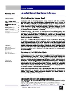
4.2. Numerical results Figure1 Figure showss the optimized 6 month routing plan from D+1 to to D+192 observing target delivery dates with times windows per each time period. In the schedule, 11 routes are generated and 9 LNG carriers are assigned to the routes. routes. Among the assigned vessels, there are 4 Type II vessels serving two demand cargoes in a route, route and another nother 7 Type I vessels deliver cargoes to single customer in a tour.

Figure 1.. LNG ship routing plan from D+1 to D+192

The measures to evaluate stochastic solutions are EVPI and VSS. EVPI is the difference between Wait and See S e (WS) and stochastic solution (RP) which expresses the value of information information. WS is defined as a probability-weighted probability weighted average of deterministic solution assuming any specific scenario realization. In this experiment, we can calculate EVPI = WS-RP RP = 1,096,784 784,497 − 1,096 096,737,898 = 46,599. On the other hand, VSS is RP minus EEV in this maximization problem which is the expected result of using mean value problem. In this test problem, EEV= EEV=1,096,737,898 096,737,898 and so we can know the value VSS=RPVSS=RP EEV=12,557 ,557 verifying the general relations between the defined measures measures; EEV ≤ RP ≤ WS in Figure 2: 2 (Birge and Louveaux, 2011). 2011)

Page 10 of 18

WS RP EEV 1,096,680

1,096,700

1,096,720

1,096,740

1,096,760

1,096,780

1,096,800

Thousands Figure 2. Optimal solutions of WS, RP and EEV

We conducted sensitivity analysis (SA) by varying the number of vessels between Type I and II vessels in a fleet: (1) SA #1-#5: SA#1is the instance that all vessels are in Type I. SA#5 is the case that all vessels are in Type II. In SA#2, 3&4, it examined the sensitivity of adding numbers of Type II vessels. As a result in Figure 3, we observed that there are significant gap between SA#1 and SA#2. This means that removing restrictions on cargo partial filling allows serving multiple customers if transportation is cost beneficial. In SA#3 and 5, there is no change because additional vessels are not necessary to maximize the profit. So, in term of long-term vessel procurement, decisions to acquire additional vessels may be critical to avoid unnecessary costs. SA#1 SA#2 SA#3 SA#4 SA#5 0

500

1,000

1,500 Millions (US $)

Figure 3. Sensitivity analysis: SA#1-5

(2) SA #6-#10: It analyzes the impact of increasing number of vessels per each vessel type from 140,000 bcm to 216,000 bcm. Figure 4 shows that increasing profit is roughly proportional to the number of Type II vessels. Hence, it is recommended to replace the current Type I vessels to Type II.

Page 11 of 18

Millions (US $)

1,200

1,000

800

SA#6-1,2,3,4,5 SA#7-1,2,3,4

600

SA#8-1,2,3,4 SA#9-1,2,3,4

400

SA#10-1

200

0 140K

160K

180K

200K

216K

Figure 4. Sensitivity analysis #6-#10

5. Conclusions In this paper, we proposed a deterministic LNG VRP model and formulated the problem using the notion of multiple vehicle routing problem. Based on this model, further extension of two-stage stochastic model was also presented applying Monte Carlo optimization techniques. Traditional LNG ship routing and scheduling problem only aims to satisfy long-term contract. However, as short-term and spot demand are rapidly increasing in LNG market, and also as LNG vessel technology can relax strict restrictions on filling limits of cargo tanks, we exactly reflected these changing environmental factors into our model. The LNG VRP model can generate six months of shipping and inventory and production schedule to serve multiple customers in a route assigning an appropriate LNG vessels. In the computational study, we showed the effectiveness of our model optimizing ship routes and schedules within the planning time horizon. As we compare the deterministic LNG VRP and its stochastic version by the measures of EVPI and VSS, we clarified the stability of stochastic solutions comparing to deterministic one. As verified in the sensitivity analysis, replacing Type I to Type II vessels in a fleet may increase more expected profit. However, it must be considered to identify how many Type II vessels are required to maximize overall profit. As stated in the model, BOR is affected by various uncertain interactive factors, and so it needs further research to develop a mathematical model to measure accurate BOR. Even though we consider many elements as deterministic components, there are still many inherent uncertainties causing severe Page 12 of 18

disruptions in LNG supply chain such as hurricane, dust storm, Tsunami, political unrest and piracy may significantly disturb planned shipping or degrades overall capability of LNG supply chain and so we expect that this will be additional research interests in the future.

Page 13 of 18

Appendices A Specification of LNG tankers No. #01 #02 #03 #04 #05 #06 #07 #08 #09 #10 #11 #12 #13 #14 #15 #16 #17 #18

Tank capacity (unit: bcm) 140,000 140,000 140,000 140,000 160,000 160,000 160,000 160,000 180,000 180,000 180,000 180,000 200,000 200,000 200,000 200,000 200,000 216,000

Daily shipping cost (unit: US dollars) 200,000 195,000 190,000 185,000 195,000 190,000 185,000 180,000 195,000 190,000 185,000 180,000 195,000 190,000 185,000 180,000 175,000 180,000

Vessel type II II II II II II I I I I I I I I I I I I

B Distance between terminals

Depot Ter.#1 Ter.#2 Ter.#3 Ter.#4

(unit: kn) Ter.#4 Ter.#5

Ter.#1

Ter.#2

Ter.#3

9,882

9,770

6,576

6,350

6,233

533

9,191

5,073

9,940

9,208

4,891

9,957

11,513

954 11,141

Page 14 of 18

C Customers demand in each time periods Time periods

No.

#1

#02 #03 #04 #05 #06 #08 #09 #10 #11 #12 #14 #15 #16 #17 #18

#2

#3

Demand (bcm) 60,000 62,500 65,000 175,000 60,000 60,000 62,500 65,000 175,000 60,000 60,000 62,500 65,000 175,000 60,000

Target date (from D+0 days) D+36 D+36 D+60 D+60 D+60 D+72 D+72 D+72 D+120 D+120 D+108 D+108 D+180 D+180 D+180

Contract type spot demand short-term long-term long-term long-term spot demand short-term long-term long-term long-term spot demand short-term long-term long-term long-term

D Other parameters Item Unit Price Storage operating cost Production cost Maximum storage level Minimum storage level BOG level Filling limit of vessels type #07- #18 Vessel speed Time window (from a target date)

Data 105 10.5 10.5 10,000 5000 [0.001, 0.0015] 0.9 19.5 ±4

Unit US dollars / bcm US dollars / bcm US dollars / bcm bcm bcm percent prcent kn days

Page 15 of 18

E Sensitivity analysis instances

No. of Type II vessels SA

Objective value

#1

140K [0,4]

160K [0,4]

180K [0,4]

200K [0,5]

216K [0,1]

7,137,500

0

0

0

0

0

#2

1,018,532,546

1

1

1

1

1

#3

1,146,492,567

2

2

2

2

1

#4

1,146,492,567

3

3

3

4

1

#5

1,146,492,567

4

4

4

5

1

#6-1

244,638,911

1

0

0

0

0

#6-2

248,293,911

0

1

0

0

0

#6-3

248,293,911

0

0

1

0

0

#6-4

252,543,911

0

0

0

1

0

#6-5

252,458,911

0

0

0

0

1

#7-1

430,355,322

2

0

0

0

0

#7-2

487,665,322

0

2

0

0

0

#7-3

487,495,322

0

0

2

0

0

#7-4

487,495,322

0

0

0

2

0

#8-1

718,026,733

3

0

0

0

0

#8-2

726,951,733

0

3

0

0

0

#8-3

726,781,733

0

0

3

0

0

#8-4

726,781,733

0

0

0

3

0

#9-1

875,478,702

4

0

0

0

0

#9-2

888,143,702

0

4

0

0

0

#9-3

726,781,733

0

0

4

0

0

#9-4

887,973702

0

0

0

4

0

#10-1

1,026,012546

0

0

0

5

0

Page 16 of 18

References Andersson, H., Christiansen, M., & Fagerholt, K. (2010). Transportation planning and inventory management in the LNG supply chain. Energy, natural resources and environmental economics, 427-439, http://dx.doi.org/10.1007/978-3-642-12067-1_24 U.S. Energy Information Administration. (2014). Annual Energy Outlook 2014 with projections to 2040. U.S. Department of Energy, available at http://www.eia.gov/forecasts/aeo/pdf/0383(2014).pdf [accessed 15 July 2014]. Birge, J. R., & Louveaux, a. F. (2011). Introduction to stochastic programming. Springer, http://dx.doi.org/10.1007/978-1-4614-0237-4 Bopp, A. E., Kannan, V. R., Palocsay, S. W., & Stevens, S. P. (1996). An optimization model for planning natural gas purchases, transportation, storage and deliverability. Omega, 24(5), 511-522, http://dx.doi.org/10.1016/0305-0483(96)00025-4. Brooke, A. K. (2010). GAMS/CPLEX 12. User notes. GAMS Development Corporation. Chatterjee, N., & Geist, J. M. (1972). Effects of stratification on boil-off rates in LNG tanks. Pipeline and Gas Journal, 199(11), 40-45. Christiansen, M., Fagerholt, K., Hasle, G., Minsaas, A., & Nygreen, B. (2009). An ocean of opportunities. OR/MS Today, pp. 24-31. Christiansen, M., Fagerholt, K., Nygreen, B., & Ronen, D. (2013). Ship routing and scheduling in the new millennium. European Journal of Operations Research, 228(3), 467-483, http://dx.doi.org/10.1016/j.ejor.2012.12.002. Coelho, L. C., & Laporte, G. (2013). The exact solution of several classes of inventory-routing problems. Computers & Operations Research, 40(2), 558-565, http://dx.doi.org/10.1016/j.cor.2012.08.012. Dobrota, Đ., Lalić, B., & Komar. (2013). Problem of Boil-off in LNG Supply Chain. Transactions on Maritime Science, 2(02), 91-100, http://dx.doi.org/10.7225/toms.v02.n02.001. Grønhaug, R., & Christiansen, M. (2009). Supply chain optimization for the liquefied natural gas business. Berlin Heidelberg: Springer, http://dx.doi.org/10.1007/978-3-540-92944-4_10. Grønhaug, R., Christiansen, M., Desaulniers, G., & Desrosiers, J. (2010). A branch and price method for a liquefied natural gas inventory routing problem. Transportation Science, 44(3), 400-415, http://dx.doi.org/10.1287/trsc.1100.0317. Halvorsen-Weare, E. E., & Fagerholt, K. (2013). Routing and scheduling in a liquefied natural gas shipping problem with inventory and berth constraints. Annals of Operations Research, 203(1), 167-186, http://dx.doi.org/10.1007/s10479-010-0794-y.

Page 17 of 18

Halvorsen-Weare, E. E., Fagerholt, K., & Rönnqvist, M. (2013). Vessel routing and scheduling under uncertainty in the liquefied natural gas business. Computers & Industrial Engineering, 64(1), 290-301, http://dx.doi.org/10.1016/j.cie.2012.10.011. Hartley, P. R., Mitchell, G., Mitchell, C., & Baker, J. A. (2013). The The Future of Long-Term LNG Contracts. University of Western Australia Business School. Huang, S. H., & Lin, P. C. (2010). A modified ant colony optimization algorithm for multi-item inventory routing problems with demand uncertainty. Transportation Research Part E: Logistics and Transportation Review, 46(5), 598-611, http://dx.doi.org/10.1016/j.tre.2010.01.006. US Department of Energy, (2005). Liquefied Natural Gas: Understanding the basic facts. US Department of Energy, available at http://energy.gov/sites/prod/files/2013/04/f0/LNG_primerupd.pdf [accessed 17 July 2014]. Miller, C. E., Tucker, A. W., & Zemlin, R. A. (1960). Integer programming formulation of traveling salesman problems. Journal of the ACM (JACM), 7(4), 326-329, http://dx.doi.org/10.1145/321043.321046. Rakke, J. G., Stålhane, M., Moe, C. R., Christiansen, M., Andersson, H. F., & Norstad, I. (2011). A rolling horizon heuristic for creating a liquefied natural gas annual delivery program. Transportation Research Part C: Emerging Technologies, 19(5), 896-911, http://dx.doi.org/10.1016/j.trc.2010.09.006. Shin, Y., Kim, J. W., Lee, H., & Hwang, C. (2003). Sloshing impact of LNG cargoes in membrance containment systems in the partially filled condition. 13th International Offshore and Polar Engineering Conference, Vol. 3, pp. 509-515. Stålhane, M., Rakke, J. G., Andersson, H., Christiansen, M., & Fagerholt, K. (2012). A construction and improvement heuristic for a liquefied natural gas inventory routing problem. Computers & Industrial Engineering, 62(1), 245-255, http://dx.doi.org/10.1016/j.cie.2011.09.011. Suvisaari, S. (2012). Delivering LNG in smaller volumes. Wärtsilä Technical Journal, 01, 21-25. Tessier, J. (2001). Operating membrane LNG carrieres-partial loading cases for 160,000 m3 vessesl and beyond. LNG13. Zakaria, M. S., Osman, K., Saadun, M. N., Manaf, M. Z., Hanafi, M., & Hafidzal, M. (2013), Computational Simulation of Boil-off Gas Formation inside Liquefied Natural Gas tank using Evaporation Model in ANSYS Fluent. Applied Mechanics and Materials, 393, 839-844 , http://dx.doi.org/10.4028/www.scientific.net/AMM.393.839.

Page 18 of 18