1
Link Budgets
Intuitive Guide to Principles of Communications www.complextoreal.com
Link Budgets You are planning a vacation. You estimate that you will need $1000 dollars to pay for the hotels, restaurants, food etc.. You start your vacation and watch the money get spent at each stop. When you get home, you pat yourself on the back for a job well done because you still have $50 left in your wallet. We do something similar with communication links, called creating a link budget. The traveler is the signal and instead of dollars it starts out with “power”. It spends its power (or attenuates, in engineering terminology) as it travels, be it wired or wireless. Just as you can use a credit card along the way for extra money infusion, the signal can get extra power infusion along the way from intermediate amplifiers such as microwave repeaters for telephone links or from satellite transponders for satellite links. The designer hopes that the signal will complete its trip with just enough power to be decoded at the receiver with the desired signal quality. In our example, we started our trip with $1000 because we wanted a budget vacation. But what if our goal was a first-class vacation with stays at five-star hotels, best shows and travel by QE2? A $1000 budget would not be enough and possibly we will need instead $5000. The quality of the trip desired determines how much money we need to take along. With signals, the quality is measured by the Bit Error Rate (BER). If we want our signal to have a low BER, we would start it out with higher power and then make sure that along the way it has enough power available at every stop to maintain this BER.
How we specify the quality of signal transmission The BER, as a measure of the signal quality, is the most important figure of merits in all link budgets. The BER is a function of a quantity called Eb/No, the bit energy per noise-density of the signal. For a QPSK signal in an additive white-gaussian-noise (AWGN) channel, the BER is given by
BER =
1 erfc 2
(
Eb / N 0
Copyright 1998 and 2002 Charan Langton
)
www.complextoreal.com
2
Link Budgets
This formula says that the BER of any signal is related to its Eb/No by the function, erfc. The function erfc, called the complimentary error function describes the cumulative probability curve of a gaussian distribution. It is found tabulated in most communications textbooks and is available as a built-in function in most math programs. The above equation when plotted has a classic waterfall shape when plotted on a log-log scale. The BER is inversely related to Eb/No. Higher Eb/No means better quality.
Figure 1 - The Bit Error rate of a signal is a function of its Eb/No Although I started out talking about signal power as a measure of signal quality, you may have noticed that I have suddenly shifted to Eb/N0. Instead of monitoring just the signal power as I said on the first page, we will actually monitor a ratio of the bit power to the noise power injected along the way. This means that in doing link budgets, we will keep track of not just the signal power and how it is getting attenuated, but also where the noise is entering into the link and how much. This dual role makes things complicated and messy because there are numerous sources of noise.
Eb/No - a measure for digital inks Eb/No is the most common parameter used to compare communication systems even when they have differing bit rates, modulations, and even media. Let’s take a closer look at the Eb/No. The quantity Eb is a measure of the Bit Energy. What is energy? The energy is the capacity to do work and energy expended per time is called power.
Copyright 1998 and 2002 Charan Langton
www.complextoreal.com
3
Link Budgets
Energy
Power
= Capacity to do work
= Energy spent /time
To compute Eb, we divide the average signal power by its bit rate.
Eb =
Pavg . Rb
This makes sense because the average power is the energy per unit time, and the bit rate is the number of bits per unit time. The division removes the units of time leaving energy per bit. We can also write the above equation in an alternate form with the amplitude-squared representing the Pavg.
A2 Eb = Rb Example 1: A signal has power of 10 watts. Its bit rate is 200 bits per second. What is its Eb? Eb = 10 Log (10) - 10 Log (200) = -13 dB In the denominator of Eb/N0, the quantity N0 is called the noise density. It is the total noise power in the frequency band of the signal divided by the bandwidth of the signal. It is measured as Watts/Hz and is the noise power in one Hz of bandwidth.
N0 =
PN BN
where PN = noise power and BN = noise bandwidth. The units are Joules.
Example 2: A signal experiences a noise power of 2 watts. The signal bandwidth is 500 Hz. (a) What is its noise power density? (b) What is its Eb/No? ( c) What would be its Eb/No if its bandwidth is 300 Hz instead of 500 Hz? Is it more or less? (a) N0 = 10 Log (2) - 10 Log (500) = -23.9 dB Case 1, Bandwidth = 500 Hz (b) Eb/N0 = -13 - (-23.9) = 10.9 dB Case 2, Bandwidth = 300 Hz (d) Eb/N0 = -13 -10 Log (2) + 10 Log (300) = 9.7 dB
Copyright 1998 and 2002 Charan Langton
www.complextoreal.com
4
Link Budgets
Note: The reason Eb/No went down in case 2 in the above example is that when we decreased the bandwidth is that the noise density has increased. The same amount of noise now occupies a smaller signal space. Eb/No decreases as the bandwidth reduced. It also decreases when we increase the bit rate. This is because Eb is inversely proportional to the bit rate. So one of the simplistic ways to improve the Eb/No of a link is to reduce its bit rate.
C/N and C/No - a measure of analog inks For analog signals, we use a quantity called C/N0 in the same way as Eb/No, where C is the signal power. C and Eb are related by the bit rate. So you will typically see C/N0 specified for the analog portions (or the passband signals) of the link and Eb/No for the digital (or the baseband) portions. C/N is simply the carrier power in the whole useable bandwidth, where C/N0 is carrier power per unit bandwidth. Let’s relate Eb/No to C/N0 and C/N. From Eq 1, we know that C = Energy per bit x bit rate = Eb x Rb, from which we get
C N0
=
Eb × Rb N0
Both C/N0 and Eb/N0 are densities so we do not need to specify the bandwidth of the signal. But to convert C/N0 to C/N, need to divide by the signal bandwidth.
E R C = b × b N N0 B In dB, we would write the above equation as
C Eb = + Rb − B N N0 and C/N0 similarly is
E C = b + Rb N0 N0 The difference between C/N and C/N0 is then only the bandwidth of the signal. And Eb/N0 is related to these quantities by the bit rate.
Copyright 1998 and 2002 Charan Langton
www.complextoreal.com
5
Link Budgets
Since we are using either Eb/No or C/N0 as our budgeting quantity, it helps to know how these quantities are impacted by some of the common parameters. We can summarize the effect on Eb/No of its various components as Variable
Action
Signal power Total noise Bandwidth Bit rate
increase increase increase increase
What happens to signal Eb/No increases ⇑ decreases ⇓ increases ⇑ decreases ⇓
What happens to signal C/N0 increases ⇑ decreases ⇓ increases ⇑ no effect
What is a link? A link consists of three parts. 1. Transmitter 2. Receiver 3. Media The very simplest form of a link equation is written as Preceived =
Power of the transmitter + Gain of the transmitting antenna + Gain of the receiving antenna - Sum of all losses
This equation of course only talks about the signal power. We have not accounted for noise yet. Now let’s talk about each of these three items.
Important things about a transmitter A transmitter receives baseband data, modulates onto a higher frequency carrier, amplifies it and broadcasts it via an antenna. The two main items that are associated with transmitters are 1. Flux Density 2. 2. EIRP Flux Density Flux Density is a measure of energy that is available for gathering from a particular source. It is called the Radio Power of a Source in Astronomy. The Sun, Moon, and stars all emit Radio Power (Flux Density). The Sun bathes us with Flux density at the rate of 10-19 Watts per square ft per unit bandwidth. (ITU however defines this unit bandwidth to be equal to 4 MHz.) The Flux Density is defined by
ψ=
GP 4π r 2
Copyright 1998 and 2002 Charan Langton
www.complextoreal.com
6
Link Budgets
where G = gain of the transmitting antenna and P = transmitter power in watts.
Figure 2 - A Transmitter consists of an amplifier and an antenna The amplifier puts out a certain amount of power and the antenna is said to have a particular gain that further amplifies this power. The combination is called the Transmitter. Usually lossy elements such as wires connect these two components in the preferred direction of radiation of the antenna. These losses are included in the quoted EIRP figure for the Transmitter. EIRP is closely related to the Flux Density. Where Flux Density is energy as measured a distance away from the source, EIRP is a measure only of the transmitted power, sort of like a Wattage rating of appliances which allows you to compare one with another. For a transmitter, this “power rating” called EIRP, is defined as the combination of EIRP = Power of transmitter x Gain of the antenna = Pamp x Gantenna
or in dB,
EIRPES = Pamp + Gantenna If you look at the equation for the Flux Density, you will see that EIRP is the numerator. EIRP is an important number for transmitters of all sorts. Spacecraft too are characterized by their EIRP which is usually in the range of about 50 dB. The Flux density is a measure of the amount of energy that is received at a distance r from a transmitter of gain G and transmit power P watts. Just as the power received is a function of the square of the amplitude of the signal, the flux density is a function of the square of the distance.
Ex. 3 What is the Flux Density received at a distance of 22,000 km away from this Earth station? (EIRP = 60 dB)
ψ = 60 - 10 log (4 π (22,000)2) = -50.2 dB
What is EIRP? EIRP is a term closely associated with a radiating source or a transmitter and is a subset of Flux Density. A very basic transmitter consists of an amplifier and an antenna.
Copyright 1998 and 2002 Charan Langton
www.complextoreal.com
7
Link Budgets
P Amplifier
G Antenna
There are two hidden assumption in EIRP. First is that the transmitter is putting out the maximum power that it can, and second, that the EIRP figure is delivered at the antenna’s boresight. So if you happen to have your antenna pointed not quite straight into the boresight of the transmitting antenna then you will not get the quoted EIRP. Ex 4. An Earth station transmits with 10 watts. Its antenna has a gain of 50 dB. (a) What is its EIRP? EIRP = 10 log 10 + 50 = 60 dBw (b). Another Earth station transmits with 8 Watts but has an antenna gain of 52 dB. Which of these would you prefer? EIRP = 10 log 8 + 52 = 61 dBw Other things being equal the second Earth Station is preferable. It has a better “rating” or the EIRP.
Important thing about Receivers is … Received Power EIRP and Flux density both tells us something about a transmitter but nothing about what is actually received. Like two people talking, the listener has to be able to hear well before communication can take place, no matter how loudly the talker talks. To compute power received by a receiver at a distance r from the source, we need to multiply the flux density with the receiving antenna’s area. Why? Because, flux density is energy per unit area per unit time. The only useable part of this energy is what is accepted by the receiving antenna. So the power received is equal to the flux density times the receiving area. We write this as Preceived = ψ Aeff The effective receiving area (not actually a physical area but strongly related to it) of any antenna is defined by
Copyright 1998 and 2002 Charan Langton
www.complextoreal.com
8
Link Budgets
λ 2GR Aeff = 4π where GR is the gain of the receiving antenna and λ is the wavelength. Now we can write the expression for computing the received power as Preceived = ψ Aeff = =
G ES PES λ 2 G R 4π r 2 4π
We can rewrite the above in dB as
4π r Preceived = EIRPES + GR - 10 Log λ
2
This equation says that if we know the gain of the receiving antenna, the EIRP of the transmitter, the operating frequency, and the distance between the two, then we can calculate the received power. The last portion of the expression above containing the ratio of the distance r to the wavelength λ , i.e. the number of wavelengths in the distance, is called the Free Space Loss (FSL).
Noise, noise everywhere So far we have been talking about signal powers, but now we must jump into a topic that causes a lot of confusion, particularly when tackling link budgets and dealing with noise figures etc. As we can see, our important parameters Eb/N0, C/N, C/N0 all have this pesky noise term on the bottom. Let’s discuss it in some detail so we can combine all the different ways of defining noise. All objects not at absolute zero emit electromagnetic radiation. The band of frequencies emitted are a function of the temperature of the object. A light bulb emits many different frequencies owing to the fact that the temperature of the filament is not uniform. However most of its radiation is in the range of infra-red light and ultraviolet frequencies which we can see and feel. The light coming from a light bulb, a jumble of frequencies, is noise that can actually be seen and appreciated. The sun puts out visible noise in the light wave frequencies among of course many others that we can not see such as X-rays and infra-red. The noise coming to us from the galaxies is typically in microwave frequencies. The moon similarly also bombards us with microwaves. The statistics of this noise is well described by quantum physics. The black body radiation problem was first solved by Max Planck in 1901. Max Planck Born in Germany, Planck is considered the originator of quantum mechanics. Planck studied at Berlin where his teachers included Helmholtz and Kirchhoff. He received his doctorate at the age of 21 in the field of thermodynamics. He taught at the University of Berlin for 38 years until he retired in 1927.
Copyright 1998 and 2002 Charan Langton
www.complextoreal.com
9
Link Budgets
He studied the distribution of energy according to wavelength. By combining the formulas of Wien and Rayleigh, Planck announced in 1900 a formula, now known as Planck's radiation formula. Very quickly he renounced classical physics by introducing the quantum of energy. At first the theory met resistance but due to the successful work of Niels Bohr in 1913, quantizing the angular momentum of the electron and calculating positions of spectral lines using the theory, it became generally accepted. Planck received the Nobel Prize for Physics in 1918. He remained in Germany during World War II through a time of the deepest personal difficulties. He lost his eldest son during World War I. In World War II, his house in Berlin was burned down in an air raid. In 1945 his other son was executed when declared guilty of complicity in a plot to kill Hitler.
The system containing the noise is modeled as a radiator of energy quanta by Max Planck. One obtains the energy radiated as a function of frequency and temperature, given by the following formula
1 1 E = hf + (h f ) 2 kT e −1 where h is Planck’s constant, f is the frequency in Hz, k is Boltzmann’s constant, and T is the temperature in degrees Kelvin. For radio, radar, and general microwave frequencies, the factor hf is quite small relative to the factor kT in the nominal range of room temperatures, say 290 Degrees Kelvin, and even down to the range of liquid nitrogen, say 77 degrees Kelvin. Thus the exponential function in the expression can be approximated by the first two terms. When this approximation is made, the denominator of the first term in the energy equation simplifies considerably, resulting in
E = kT +
hf 2
Again applying the approximation hf