sal11586_ch08.qxd
10/10/03
10:12 AM
Page 336
Chapter
8
Linear Programming CHAPTER OUTLINE
KEY TERMS Linear programming Production process Feasible region Optimal solution Objective function Inequality constraints Nonnegativity constraints Decision variables Binding constraints Slack variable Simplex method Primal problem Dual problem Shadow price Duality theorem Logistic management
8-1 Meaning, Assumptions, and Applications of Linear Programming • The Meaning and Assumptions of Linear Programming • Applications of Linear Programming 8-2 Some Basic Linear Programming Concepts • Production Processes and Isoquants in Linear Programming • The Optimal Mix of Production Processes 8-3 Procedure Used in Formulating and Solving Linear Programming Problems 8-4 Linear Programming: Profit Maximization • Formulation of the Profit Maximization Linear Programming Problem • Graphic Solution of the Profit Maximization Problem • Extreme Points and the Simplex Method • Algebraic Solution of the Profit Maximization Problem • Case Study 8-1: Maximizing Profits in Blending Aviation Gasoline and Military Logistics by Linear Programming • Case Study 8-2: Linear Programming as a Tool of Portfolio Management 8-5 Linear Programming: Cost Minimization • Formulation of the Cost Minimization Linear Programming Problem • Graphic Solution of the Cost Minimization Problem • Algebraic Solution of the Cost Minimization Problem • Case Study 8-3: Cost Minimization Model for Warehouse Distribution Systems and Supply Chain Management 8-6 The Dual Problem and Shadow Prices • The Meaning of Dual and Shadow Prices • The Dual of Profit Maximization • The Dual of Cost Minimization • Case Study 8-4: Shadow Prices in Closing an Airfield in a Forest Pest Control Program 8-7 Linear Programming and Logistics in the Global Economy • Case Study 8-5: Measuring the Pure Efficiency of Operating Units • Case Study 8-6: Logistics at National Semiconductor, Saturn, and Compaq 8-8 Actual Solution of Linear Programming Problems on Personal Computers Summary • Discussion Questions • Problems • Supplementary Readings • Internet Site Addresses Integrating Case Study Three: Production and Cost Functions in the Petroleum Industry, Duality, and Linear Programming
336
sal11586_ch08.qxd
10/10/03
10:12 AM
Page 337
Chapter 8
Linear Programming
n this chapter we introduce linear programming. This is a powerful technique that is often used by large corporations, not-for-profit organizations, and government agencies to analyze complex production, commercial, financial, and other activities. The chapter begins by examining the meaning of “linear programming,” the assumptions on which it is based, and some of its applications. We then present the basic concepts of linear programming and examine its relationship to the production and cost theories discussed in Chapters 6 and 7. Subsequently, we show how linear programming can be used to solve complex constrained profit maximization and cost minimization problems, and we estimate the economic value or shadow price of each input. The theory is reinforced with six case studies of real-world applications of linear programming. Also discussed in this chapter is the use of linear programming and logistics in the world economy today. Finally, we show how to solve linear programming problems on personal computers using one of the simplest and most popular software programs.
I
8-1 MEANING, ASSUMPTIONS, AND APPLICATIONS OF LINEAR PROGRAMMING In this section we define linear programming and examine its origin, specify the assumptions on which it rests, and examine some of the situations to which it has been successfully applied.
The Meaning and Assumptions of Linear Programming Linear programming is a mathematical technique for solving constrained maximization and minimization problems when there are many constraints and the objective function to be optimized, as well as the constraints faced, are linear (i.e., can be represented by straight lines). Linear programming was developed by the Russian mathematician L. V. Kantorovich in 1939 and extended by the American mathematician G. B. Dantzig in 1947. Its acceptance and usefulness have been greatly enhanced by the advent of powerful computers, since the technique often requires vast calculations. Firms and other organizations face many constraints in achieving their goals of profit maximization, cost minimization, or other objectives. With only one constraint, the problem can easily be solved with the traditional techniques presented in the previous two chapters. For example, we saw in Chapter 6 that in order to maximize output (i.e., reach a given isoquant) subject to a given cost constraint (isocost), the firm should produce at the point where the isoquant is tangent to the firm’s isocost. Similarly, in order to minimize the cost of producing a given level of output, the firm seeks the lowest isocost that is tangent to the given isoquant. In the real world, however, firms and other organizations often face numerous constraints. For example, in the short run or operational period, a firm may not be able to hire more labor
337
sal11586_ch08.qxd
338
10/10/03
Part 3
10:12 AM
Page 338
Production and Cost Analysis
with some type of specialized skill, obtain more than a specified quantity of some raw material, or purchase some advanced equipment, and it may be bound by contractual agreements to supply a minimum quantity of certain products, to keep labor employed for a minimum number of hours, to abide by some pollution regulations, and so on. To solve such constrained optimization problems, traditional methods break down and linear programming must be used. Linear programming is based on the assumption that the objective function that the organization seeks to optimize (i.e., maximize or minimize), as well as the constraints that it faces, are linear and can be represented graphically by straight lines. This means that we assume that input and output prices are constant, that we have constant returns to scale, and that production can take place with limited technologically fixed input combinations. Constant input prices and constant returns to scale mean that average and marginal costs are constant and equal (i.e., they are linear). With constant output prices, the profit per unit is constant, and the profit function that the firm may seek to maximize is linear. Similarly, the total cost function that the firm may seek to minimize is also linear.1 The limited technologically fixed input combinations that a firm can use to produce each commodity result in isoquants that are not smooth as shown in Chapter 6 but will be made up of straight line segments (as shown in the next section). Since firms and other organizations often face a number of constraints, and the objective function that they seek to optimize as well as the constraints that they face are often linear over the relevant range of operation, linear programming is very useful.
Applications of Linear Programming Linear programming has been applied to a wide variety of constrained optimization problems. Some of these are 1. Optimal process selection. Most products can be manufactured by using a number of processes, each requiring a different technology and combination of inputs. Given input prices and the quantity of the commodity that the firm wants to produce, linear programming can be used to determine the optimal combination of processes needed to produce the desired level and output at the lowest possible cost, subject to the labor, capital, and other constraints that the firm may face. This type of problem is examined in Section 8-2. 2. Optimal product mix. In the real world, most firms produce a variety of products rather than a single one and must determine how to best use their plants, labor, and other inputs to produce the combination or mix of
1
The total profit function is obtained by multiplying the profit per unit of output by the number of units of output and summing these products for all the commodities produced. The total cost function is obtained by multiplying the price of each input by the quantity of the input used and summing these products over all the inputs used.
sal11586_ch08.qxd
10/10/03
10:12 AM
Page 339
Chapter 8
Linear Programming
products that maximizes their total profits subject to the constraints they face. For example, the production of a particular commodity may lead to the highest profit per unit but may not use all the firm’s resources. The unused resources can be used to produce another commodity, but this product mix may not lead to overall profit maximization for the firm as a whole. The product mix that would lead to profit maximization while satisfying all the constraints under which the firm is operating can be determined by linear programming. This type of problem is examined in Section 8-3, and a real-world example of it is given in Case Study 8-1. 3. Satisfying minimum product requirements. Production often requires that certain minimum product requirements be met at minimum cost. For example, the manager of a college dining hall may be required to prepare meals that satisfy the minimum daily requirements of protein, minerals, and vitamins at a minimum cost. Since different foods contain various proportions of the various nutrients and have different prices, the problem can be complex. This problem, however, can be solved easily by linear programming by specifying the total cost function that the manager seeks to minimize and the various constraints that he or she must meet or satisfy. The same type of problem is faced by a chicken farmer who wants to minimize the cost of feeding chickens the minimum daily requirements of certain nutrients; a petroleum firm that wants to minimize the cost of producing a gasoline of a particular octane subject to its refining, transportation, marketing, and exploration requirements; a producer of a particular type of bolt joints who may want to minimize production costs, subject to its labor, capital, raw materials, and other constraints. This type of problem is examined in Section 8-4, and a real-world example of it is given in Case Study 8-2. 4. Long-run capacity planning. An important question that firms seek to answer is how much contribution to profit each unit of the various inputs makes. If this exceeds the price that the firm must pay for the input, this is an indication that the firm’s total profits would increase by hiring more of the input. On the other hand, if the input is underused, this means that some units of the input need not be hired or can be sold to other firms without affecting the firm’s output. Thus, determining the marginal contribution (shadow price) of an input to production and profits can be very useful to the firm in its investment decisions and future profitability. 5. Other specific applications of linear programming. Linear programming has also been applied to determine (a) the least-cost route for shipping commodities from plants in different locations to warehouses in other locations, and from there to different markets (the so-called transportation problem); (b) the best combination of operating schedules, payload, cruising altitude, speed, and seating configurations for airlines; (c) the best combination of logs, plywood, and paper that a forest products company can produce from given supplies of logs and milling capacity; (d) the distribution of a given advertising budget among TV, radio, magazines, newspapers, billboards, and
339
sal11586_ch08.qxd
340
10/10/03
Part 3
10:12 AM
Page 340
Production and Cost Analysis
other forms of promotion to minimize the cost of reaching a specific number of customers in a particular socioeconomic group; (e) the best routing of millions of telephone calls over long distances; (f ) the best portfolio of securities to hold to maximize returns subject to constraints based on liquidity, risk, and available funds; (g) the best way to allocate available personnel to various activities, and so on. Although these problems are different in nature, they all basically involve constrained optimization, and they can all be solved and have been solved by linear programming. This clearly points out the great versatility and usefulness of this technique. While linear programming can be complex and is usually conducted by the use of computers, it is important to understand its basic principles and how to interpret its results. To this end, we present next some basic linear programming concepts before moving on to more complex and realistic cases.
8-2 SOME BASIC LINEAR PROGRAMMING CONCEPTS Though linear programming is applicable in a wide variety of contexts, it has been more fully developed and more frequently applied in production decisions. Production analysis also represents an excellent point of departure for introducing some basic linear programming concepts. We begin by defining the meaning of a production process and deriving isoquants. By then bringing in the production constraints, we show how the firm can determine the optimal mix of production processes to use in order to maximize output.
Production Processes and Isoquants in Linear Programming As pointed out in Section 8-1, one of the basic assumptions of linear programming is that a particular commodity can be produced with only a limited number of input combinations. Each of these input combinations or ratios is called a production process or activity and can be represented by a straight line ray from the origin in the input space. For example, the left panel of Figure 8-1 shows that a particular commodity can be produced with three processes, each using a particular combination of labor (L) and capital (K ). These are: process 1 with K/L � 2, process 2 with K/L � 1, and process 3 with K/L � 12. Each of these processes is represented by the ray from the origin with slope equal to the particular K/L ratio used. Process 1 uses 2 units of capital for each unit of labor used, process 2 uses 1K for each 1L used, and process 3 uses 0.5K for each 1L used. By joining points of equal output on the rays of processes, we define the isoquant for the particular level of output of the commodity. These isoquants will be made up of straight-line segments and have kinks (rather than being
sal11586_ch08.qxd
10/10/03
10:12 AM
Page 341
Chapter 8
FIGURE 8-1
Linear Programming
341
The Firm’s Production Processes and Isoquants
Capital (K )
K Process 1 (K/ L = 2)
Process 1
12
D
12 Process 2 (K/ L = 1)
8
Process 2
20
8
6
Process 3 (K/ L = 12 )
4
E
0
2
4
6
8
10
12
Labor (L)
Process 3
A
6
F
10
0Q
4 3
B C
2 0
0Q
0 0
3 4
6
8
12
L
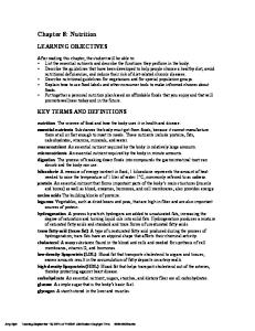
The left panel shows production process 1 using K/L � 2, process 2 using K/L � 1, and process 3 using K/L � 12 that a firm can use to produce a particular commodity. The right panel shows that 100 units of output (100Q) can be produced with 6K and 3L (point A), 4K and 4L (point B), or 6L and 3K (point C). Joining these points, we get the isoquant for 100Q. Because of constant returns to scale, using twice as many inputs along each production process (ray) results in twice as much output. Joining such points, we get the isoquant for 200Q.
smooth as in Chapter 6). For example, the right panel of Figure 8-1 shows that 100 units of output (100Q) can be produced with process 1 at point A (i.e., by using 3L and 6K), with process 2 at point B (by using 4L and 4K), or with process 3 at point C (with 6L and 3K). By joining these points, we get the isoquant for 100Q. Note that the isoquant is not smooth but has kinks at points A, B, and C.2 Furthermore, since we have constant returns to scale, the isoquant for twice as much output (that is, 200Q) is determined by using twice as much of each input with each process. This defines the isoquant for 200Q with kinks at points D (6L, 12K), E (8L, 8K), and F (12L, 6K). Note that corresponding segments on the isoquant for 100Q and 200Q are parallel.
The Optimal Mix of Production Processes If the firm faced only one constraint, such as isocost line GH in the left panel of Figure 8-2, the feasible region, or the area of attainable input combinations, is represented by shaded triangle 0JN. That is, the firm can purchase any combination of labor and capital on or below isocost line GH. But since 2
The greater the number of processes available to produce a particular commodity, the less pronounced are these kinks and the more the isoquants approach the smooth curves assumed in Chapter 6.
sal11586_ch08.qxd
342
10/10/03
Part 3
10:13 AM
Page 342
Production and Cost Analysis
Feasible Region and Optimal Solution
FIGURE 8-2 K
K
G
16
1
1
D
12
D
12 2
J E
8
200
6
2
S E
3
Q
A
6
F N
4
R
10
200
3
Q F
4
B
T
2 H 0 0
2
4
6
8
12
16
L
0 0
3 4
7
12
L
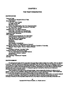
With isocost line GH in the left panel, the feasible region is shaded triangle 0J N, and the optimal solution is at point E where the firm uses 8L and 8K and produces 200Q. The right panel shows that if the firm faces no cost constraint but has available only 7L and 10K, the feasible region is shaded area 0RST and the optimal solution is at point S where the firm produces 200Q. To reach point S, the firm produces 100Q with process 1 (0A) and 100Q with process 2 (0B � AS).
no production process is available that is more capital intensive than process 1 (i.e., which involves a K/L higher than 2) or less capital intensive than process 3 (i.e., with K/L smaller than 12), the feasible region is restricted to the shaded area 0JN. The best or optimal solution is at point E where the feasible region reaches the isoquant for 200Q (the highest possible). Thus, the firm produces the 200 units of output with process 2 by using 8L and 8K. The right panel of Figure 8-2 extends the analysis to the case where the firm faces no cost constraint but has available only 7L and 10K for the period of time under consideration. The feasible region is then given by shaded area 0RST in the figure. That is, only those labor-capital combinations in shaded area 0RST are relevant. The maximum output that the firm can produce is 200Q and is given by point S. That is, the isoquant for 200Q is the highest that the firm can reach with the constraints it faces. To reach point S, the firm will have to produce 100Q with process 1 (0A) and 100Q with process 2 (0B � AS).3 Note that when the firm faced the single isocost constraint (GH in the left panel of Figure 8-2), the firm used only one process (process 2) to reach the optimum. When the firm faced two constraints (the right panel), the firm 3 0A and 0B are called “vectors.” Thus, the above is an example of vector analysis, whereby vector 0S (not shown in the right panel of Figure 8-2) is equal to the sum of vectors 0A and 0B.
sal11586_ch08.qxd
10/10/03
10:13 AM
Page 343
Chapter 8
Linear Programming
required two processes to reach the optimum. From this, we can generalize and conclude that to reach the optimal solution, a firm will require no more processes than the number of constraints that the firm faces. Sometimes fewer processes will do. For example, if the firm could use no more than 6L and 12K, the optimum would be at point D (200Q), and this is reached with process 1 alone (see the left panel of Figure 8-2).4 From the left panel of Figure 8-2 we can also see that if the ratio of the wage rate (w) to the rental price of capital (r) increased (so that isocost line GH became steeper), the optimal solution would remain at point E as long as the GH isocost (constraint) line remained flatter than segment DE on the isoquant for 200Q. If w/r rose so that isocost GH coincided with segment DE, the firm could reach isoquant 200Q with process 1, process 2, or any combination of process 1 and process 2 that would allow the firm to reach a point on segment DE. If w/r rose still further, the firm would reach the optimal solution (maximum output) at point D (see the figure).
8-3 PROCEDURE USED IN FORMULATING AND SOLVING LINEAR PROGRAMMING PROBLEMS The most difficult aspect of solving a constrained optimization problem by linear programming is to formulate or state the problem in a linear programming format or framework. The actual solution to the problem is then straightforward. Simple linear programming problems with only a few variables are easily solved graphically or algebraically. More complex problems are invariably solved by the use of computers. It is important, however, to know the process by which even the most complex linear programming problems are formulated and solved and how the results are interpreted. To show this, we begin by defining some important terms and then using them to outline the steps to follow in formulating and solving linear programming problems. The function to be optimized in linear programming is called the objective function. This usually refers to profit maximization or cost minimization. In linear programming problems, constraints are given by inequalities (called inequality constraints). The reason is that the firm can often use up to, but not more than, specified quantities of some inputs, or the firm must meet some minimum requirement. In addition, there are nonnegativity constraints on the solution to indicate that the firm cannot produce a negative output or use a negative quantity of any input. The quantities of each
4
To reach any point on an isoquant between two adjacent production processes, we use the process to which the point is closer, in proportion to 1 minus the distance of the point from the process (ray). For example, if point S were one-quarter of the distance DE from point D along the isoquant for 200Q, the firm would produce 1 � 14 � 34 of the 200Q (that is, 150Q) with process 1 and the remaining 14 with process 2 (see the figure). The amount of each input that is used in each process is then proportional to the output produced by each process.
343
sal11586_ch08.qxd
344
10/10/03
Part 3
10:13 AM
Page 344
Production and Cost Analysis
product to produce in order to maximize profits or inputs to use to minimize costs are called decision variables. The steps followed in solving a linear programming problem are: 1. Express the objective function of the problem as an equation and the constraints as inequalities. 2. Graph the inequality constraints, and define the feasible region. 3. Graph the objective function as a series of isoprofit (i.e., equal profit) or isocost lines, one for each level of profit or costs, respectively. 4. Find the optimal solution (i.e., the values of the decision variables) at the extreme point or corner of the feasible region that touches the highest isoprofit line or the lowest isocost line. This represents the optimal solution to the problem subject to the constraints faced. In the next section we will elaborate on these steps as we apply them to formulate and solve a specific profit maximization problem. In the following section, we will apply the same general procedure to solve a cost minimization problem.
8-4 LINEAR PROGRAMMING: PROFIT MAXIMIZATION In this section, we follow the steps outlined in the previous section to formulate and solve a specific profit maximization problem, first graphically and then algebraically. We will also examine the case of multiple solutions.
Formulation of the Profit Maximization Linear Programming Problem Most firms produce more than one product, and a crucial question to which they seek an answer is how much of each product (the decision variables) the firm should produce in order to maximize profits. Usually, firms also face many constraints on the availability of the inputs they use in their production activities. The problem is then to determine the output mix that maximizes the firm’s total profit subject to the input constraints it faces. In order to show the solution of a profit maximization problem graphically, we assume that the firm produces only two products: product X and product Y. Each unit of product X contributes $30 to profit and to covering overhead (fixed) costs, and each unit of product Y contributes $40.5 Suppose also that in order to produce each unit of product X and product Y, the firm 5
The contribution to profit and overhead costs made by each unit of the product is equal to the difference between the selling price of the product and its average variable cost. Since the total fixed costs of the firm are constant, however, maximizing the total contribution to profit and to overhead costs made by the product mix chosen also maximizes the total profits of the firm.
sal11586_ch08.qxd
10/10/03
10:13 AM
Page 345
Chapter 8
TABLE 8-1
Input Requirements and Availability for Producing Products X and Y Quantities of Inputs Required per Unit of Output
Input A B C
Linear Programming
Quantities of Inputs Available per Time Period
Product X
Product Y
Total
1 0.5 0
1 1 0.5
7 5 2
requires inputs A, B, and C in the proportions indicated in Table 8-1. That is, each unit of product X requires 1 unit of input A, one-half unit of input B, and no input C, while 1 unit of product Y requires 1A, 1B, and 0.5C. Table 8-1 also shows that the firm has available only 7 units of input A, 5 units of input B, and 2 units of input C per time period. The firm then wants to determine how to use the available inputs to produce the mix of products X and Y that maximizes its total profits. The first step in solving a linear programming problem is to express the objective function as an equation and the constraints as inequalities. Since each unit of product X contributes $30 to profit and overhead costs and each unit of product Y contributes $40, the objective function that the firm seeks to maximize is � � $30QX � $40QY
(8-1)
where � is the total contribution to profit and overhead costs faced by the firm (henceforth simply called the “profit function”), and QX and QY refer, respectively, to the quantities of product X and product Y that the firm produces. Thus, Equation 8-1 postulates that the total profit (contribution) function of the firm equals the per-unit profit contribution of product X times the quantity of product X produced plus the per-unit profit contribution of product Y times the quantity of product Y that the firm produces. Let us now go on to express the constraints of the problem as inequalities. From the first row of Table 8-1, we know that 1 unit of input A is required to produce each unit of product X and product Y and that only 7 units of input A are available to the firm per period of time. Thus, the constraint imposed on the firm’s production by input A can be expressed as 1QX � 1QY � 7
(8-2)
That is, the 1 unit of input A required to produce each unit of product X times the quantity of product X produced plus the 1 unit of input A required to produce each unit of product Y times the quantity of product Y produced must be equal to or smaller than the 7 units of input A available to the firm.
345
sal11586_ch08.qxd
346
10/10/03
Part 3
10:13 AM
Page 346
Production and Cost Analysis
The inequality sign indicates that the firm can use up to, but no more than, the 7 units of input A available to it to produce products X and Y. The firm can use less than 7 units of input A, but it cannot use more. From the second row of Table 8-1, we know that one-half unit of input B is required to produce each unit of product X and 1 unit of input B is required to produce each unit of product Y, and only 5 units of input B are available to the firm per period of time. The quantity of input B required in the production of product X is then 0.5QX, while the quantity of input B required in the production of product Y is 1QY and the sum of 0.5QX and 1QY can be equal to, but it cannot be more than, the 5 units of input B available to the firm per time period. Thus, the constraint associated with input B is 0.5QX � 1QY � 5
(8-3)
From the third row in Table 8-1, we see that input C is not used in the production of product X, one-half unit of input C is required to produce each unit of product Y, and only 2 units of input C are available to the firm per time period. Thus, the constraint imposed on production by input C is 0.5QY � 2
(8-4)
In order for the solution to the linear programming problem to make economic sense, however, we must also impose nonnegativity constraints on the output of products X and Y. The reason for this is that the firm can produce zero units of either product, but it cannot produce a negative quantity of either product (or use a negative quantity of either input). The requirement that QX and QY (as well as that the quantity used of each input) be nonnegative can be expressed as QX � 0
QY � 0
We can now summarize the linear programming formulation of the above problem as follows: Maximize Subject to
� � $30QX � $40QY 1QX � 1QY � 7 0.5QX � 1QY � 5 0.5QY � 2 QX, QY � 0
(objective function) (input A constraint) (input B constraint) (input C constraint) (nonnegativity constraint)
Graphic Solution of the Profit Maximization Problem The next step in solving the linear programming problem is to treat the inequality constraints of the problem as equations, graph them, and define the feasible region. These are shown in Figure 8-3. Figure 8-3a shows the graph of the constraint imposed on the production of products X and Y by input A. Treating inequality constraint 8-2 for input A as an equation (i.e., disregarding the inequality sign for the moment), we have 1QX � 1QY � 7. With 7
sal11586_ch08.qxd
10/10/03
10:13 AM
Page 347
Chapter 8
347
Linear Programming
Feasible Region, Isoprofit Lines, and Profit Maximization
FIGURE 8-3
QY 7
7 Constraint on input A 1QX + 1QY � 7
Quantity of Y (QY)
6
Constraint on input A 1QX + 1QY � 7
6
5
5
4
4
3
3
2
2
G
F
Constraint on input C 0.5QY � 2 E Constraint on input B 0.5QX + 1QY � 5
Feasible region 1
1
0
0
D 0
1
2
3
4
5
6
0
7
1
2
3
4
5
Quantity of X (QX) (a)
6
7
8
9
10 QX
(b)
QY 7.5
QY H
6
6
π=
4.5
π= π= 2
$3 00
G
4
$2 40
F E
3
$1 80
D
0
0 0
2
4
6 (c)
8
10 QX
0
2
4
7
J 8 QX
(d)
The shaded area in part a shows the inequality constraint from input A. The shaded area in part b shows the feasible region, where all the inequality constraints are simultaneously satisfied. Part c shows the isoprofit lines for � � $180, � � $240, and � � $300. All three isoprofit lines have an absolute slope of $30/$40 or 34, which is the ratio of the contribution of each unit of X and Y to the profit and overhead costs of the firm. Part d shows that � is maximized at point E where the feasible region touches isoprofit line HJ (the highest possible) when the firm produces 4X and 3Y so that � � $30(40) � $40(3) � $240.
sal11586_ch08.qxd
348
10/10/03
Part 3
10:13 AM
Page 348
Production and Cost Analysis
units of input A available, the firm could produce 7 units of product X (that is, 7X) and no units of product Y, 7Y and 0X, or any combination of X and Y on the line joining these two points. Since the firm could use an amount of input A equal to or smaller than the 7 units available to it, inequality constraint 8-2 refers to all the combinations of X and Y on the line and in the entire shaded region below the line (see Figure 8-3a). In Figure 8-3b we have limited the feasible region further by considering the constraints imposed by the availability of inputs B and C. The constraint on input B can be expressed as the equation 0.5QX � 1QY � 5. Thus, if QX � 0, QY � 5, and if QY � 0, QX � 10. All the combinations of product X and product Y falling on or to the left of the line connecting these two points represent the inequality constraint 8-3 for input B. The horizontal line at QY � 4 represents the constraint imposed by input C. Since input C is not used in the production of product X, there is no constraint imposed by input C on the production of product X. Since 0.5 unit of input C is required to produce each unit of product Y and only 2 units of input C are available to the firm, the maximum quantity of product Y that the firm can produce is 4 units. Thus, the constraint imposed by input C is represented by all the points on or below the horizontal line at QY � 4. Together with the nonnegativity constraints on QX and QY, we can, therefore, define the feasible region as the shaded region of 0DEFG, for which all the inequality constraints facing the firm are satisfied simultaneously. The third step in solving the linear programming problem is to graph the objective function of the firm as a series of isoprofit (or equal) profit lines. Figure 8-3c shows the isoprofit lines for � equal to $180, $240, and $300. The lowest isoprofit line in Figure 8-3c is obtained by substituting $180 for � into the equation for the objective function and then solving for QY. Substituting $180 for � in the objective function, we have $180 � $30QX � $40QY Solving for QY, we obtain QY �
� �
$180 $30 � Q $40 $40 X
(8-5)
Thus, when QX � 0, QY � $180/$40 � 4.5 and the slope of the isoprofit line is �$30/$40, or �43. This isoprofit line shows all the combinations of products X and Y that result in � � $180. Similarly, the equation of the isoprofit line for � � $240 is QY �
� �
$240 $30 Q � $40 $40 X
(8-6)
for which QY � 6 when QX � 0 and the slope is �34. Finally, the isoprofit equation for � � $300 is QY �
� �
$300 $30 � Q $40 $40 X
(8-7)
sal11586_ch08.qxd
10/10/03
10:13 AM
Page 349
Chapter 8
Linear Programming
for which QY � 7.5 when QX � 0 and the slope is �34. Note that the slopes of all isoprofit lines are the same (i.e., the isoprofit lines are parallel) and are equal to �1 times the ratio of the profit contribution of product X to the profit contribution of product Y (that is, �$30/$40 � �34). The fourth and final step in solving the linear programming problem is to determine the mix of products X and Y (the decision variables) that the firm should produce in order to reach the highest isoprofit line. This is obtained by superimposing the isoprofit lines shown in Figure 8-3c on the feasible region shown in Figure 8-3b. This is done in Figure 8-3d, which shows that the highest isoprofit line that the firm can reach subject to the constraints it faces is HJ. This is reached at point E where the firm produces 4X and 3Y and the total contribution to profit (�) is maximum at $30(4) � $40(3) � $240. Note that point E is at the intersection of the constraint lines for inputs A and B but below the constraint line for input C. This means that inputs A and B are fully utilized, while input C is not.6 In the terminology of linear programming, we then say that inputs A and B are binding constraints, while input C is nonbinding or is a slack variable.7
Extreme Points and the Simplex Method In the previous section, we showed that the firm’s optimal or profit maximization product mix is given at point E, a corner of the feasible region.8 This example illustrates a basic theorem of linear programming. This is that in searching for the optimal solution, we need to examine and compare the levels of � at only the extreme points (corners) of the feasible region and can ignore all other points inside or on the borders of the feasible region. That is, with a linear objective function and linear input constraints, the optimal solution will always occur at one of the corners. In the unusual event that the isoprofit lines have the same slope as one of the segments of the feasible region, then all the product mixes along that segment will result in the same maximum value, and we have multiple optimal solutions. Since these include the two corners defining the segment, the rule that in order to find the optimal or profit-maximizing product mix, we only need to examine and compare the value of � at the corners of the feasible region holds up. Figure 8-4 shows the case of multiple optimal solutions. In the figure, the new isoprofit line H�J � ($240 � $24QX � $48QY) has the absolute slope of $24/$48 � 12, the same as segment EF of the feasible region. Thus, all the product mixes along EF, including those at corner points E and F, result in the same value of � � $240. For example, at point M (3X, 3.5Y ) on EF, 6 From Figure 8-3b, we can see that at point E only 112 out of the 2 units of input C available to the firm per time period are used. 7 We will return to this in the algebraic solution to this problem in the following subsection and in our discussion of the dual problem and shadow prices in Section 8-6. 8 At the other corners of the feasible region, the values of � are as follows: at corner point D(7, 0), � � $30(7) � $210; at point F (2, 4), � � $30(2) � $40(4) � $220; at point G (0, 4), � � $40(4) � $160; and at the origin (0, 0), � � 0.
349
sal11586_ch08.qxd
350
10/10/03
Part 3
10:13 AM
Page 350
Production and Cost Analysis
Multiple Optimal Solutions
FIGURE 8-4 QY
H
6
H’
5
G
4 3.5 3
$240 = $30QX + $40QY
F E
M
$240 = $24QX + $48QY
2 1
G
0 0
2
3
4
7
J 8
J’ 10
QX
The new isoprofit line H�J� ($240 � $24QX � $48QY) has the same absolute slope of $24/$48 � 12 as segment EF of the feasible region. Thus, all the product mixes along EF, such as those indicated at point M and at corner points E and F, result in the same value of � � $240.
� � $24(3) � $48(3.5) � $240. Since � � $240 at corner point E and at corner point F also, we can find the optimal solution of the problem by examining only the corners of the feasible region, even in a case such as this one where there are multiple optimal points.9 The ability to determine the optimal solution by examining only the extreme or corner points of the feasible region greatly reduces the calculations necessary to solve linear programming problems that are too large to solve graphically. These large linear programming problems are invariably solved by computers. All the computer programs available for solving linear programming problems start by arbitrarily picking one corner and calculating the value of the objective function at that corner, and then systematically moving to other corners that result in higher profits until they find no corner with higher profits. This is referred to as the “extreme-point theorem,” and the At corner point E (4, 3), � � $24(4) � $48(3) � $240; at corner point F (2, 4), � � $24(2) � $48(4) � $240. Sometimes a constraint may be redundant. This occurs when the feasible region is defined only by the other constraints of the problem. For example, if the constraint equation for input C had been 0.5QY � 3, the constraint line for input C would have been a horizontal straight line at QY � 6 and fallen outside the feasible region of the problem (which in that case would have been defined by the constraint lines for inputs A and B only—see Figure 8-3b). There are other cases where a constraint may make the solution of the problem impossible. In that case (called “degeneracy”), the constraints have to be modified in order to obtain a solution to the problem (see Problem 7).
9
sal11586_ch08.qxd
10/10/03
10:13 AM
Page 351
Chapter 8
FIGURE 8-5
Linear Programming
351
Algebraic Determination of the Corners of the Feasible Region
QY 7 Constraint on input A 1QX + 1QY 7 5 4
Constraint on input C 0.5QY 2
G (0,4) F (2,4)
E (4,3)
3
Constraint on input B 0.5QX + 1QY 5 D (7,0)
0 0
2
4
7
10
QX
The quantity of products X and Y (that is, QX and QY) at corner point D is obtained by substituting QY � 0 (along the QX axis) into the constraint equation for input A. QX and QY at corner point E are obtained by solving simultaneously the constraint equations for inputs A and B. QX and QY at point F are obtained by solving simultaneously the equations for constraints B and C. Corner point G can be dismissed outright because it involves the same QY as at point F but has QX � 0. The origin can also be dismissed since QX � QY � � � 0.
method of solution is called the simplex method. The algebraic solution to the linear programming problem examined next provides an idea of how the computer proceeds in solving the problem.10
Algebraic Solution of the Profit Maximization Problem The profit maximization linear programming problem that was solved graphically earlier can also be solved algebraically by identifying (algebraically) the corners of the feasible region and then comparing the profits at each corner. Since each corner is formed by the intersection of two constraint lines, the coordinates of the intersection point (i.e., the value of ) QX and QY at the corner can be found by solving simultaneously the equations of the two intersecting lines. This can be seen in Figure 8-5 (which is similar to Figure 8-3b). 10
In 1984, N. Karmarkar of Bell Labs discovered a new algorithm or mathematical formula that solved very large linear programming problems 50 to 100 times faster than with the simplex method. However, most routine linear programming problems are still being solved with the simplex method. See “The Startling Discovery Bell Labs Kept in the Shadows,” Business Week, September 21, 1987, pp. 69–76, and C. E. Downing and J. L. Ringuest, “An Experimental Evaluation of the Efficacy of Four Multiobjective Linear Programming Algorithms,” European Journal of Operational Research, February 1998, pp. 549–558.
sal11586_ch08.qxd
352
10/10/03
Part 3
10:13 AM
Page 352
Production and Cost Analysis
In Figure 8-5, only corner points D, E, and F need to be considered. While the origin is also a corner point of the feasible region, profits are zero at this point because QX � QY � 0. Corner point G (0X, 4Y ) can also be dismissed because it refers to the same output of product Y as at corner point F but to less of product X. This leaves only corner points D, E, and F to be evaluated. Since corner point D is formed by the intersection of the constraint line for input A with the horizontal axis (along which QY � 0, see Figure 8-5), the quantity of product X (that is, QX) at corner point D is obtained by substituting QY � 0 into the equation for constraint A. That is, substituting QY � 0 into 1QX � 1QY � 7 we get
QX � 7
Thus, at point D, QX � 7 and QY � 0. Corner point E is formed by the intersection of the constraint lines for inputs A and B (see Figure 8-5), which are, respectively, 1QX � 1QY � 7 and 0.5QX � 1QY � 5 Subtracting the second equation from the first, we have 1QX � 1QY � 7 0.5QX � 1QY � 5 0.5QX
�2
so that QX � 4. Substituting QX � 4 into the first of the two equations, we get QY � 3. Thus, QX � 4 and QY � 3 at corner point E. These are the same values of QX and QY determined graphically in Figure 8-3b. Finally, corner point F is formed by the intersection of the constraint lines for inputs B and C, which are, respectively, 0.5QX � 1QY � 5 and 0.5QY � 2 Substituting QY � 4 from the second equation into the first equation, we have 0.5QX � 4 � 5 so that QX � 2. Thus at corner point F, QX � 2 and QY � 4 (the same as obtained graphically in Figure 8-3b). By substituting the values of QX and QY (the decision variables) at each corner of the feasible region into the objective function, we can then determine the firm’s total profit contribution (�) at each corner. These are shown in Table 8-2, which (for the sake of completeness) also shows the levels of profit at the origin and at point G. The optimal or profit-maximizing point is
sal11586_ch08.qxd
10/10/03
10:13 AM
Page 353
Chapter 8
TABLE 8-2
Linear Programming
Outputs of Products X and Y, and Profits at Each Corner of the Feasible Region
Corner Point
QX
QY
$30QX � $40QY
Profit
0 D *E F G
0 7 4 2 0
0 0 3 4 4
$30(0) � $40(0) $30(7) � $40(0) $30(4) � $40(3) $30(2) � $40(4) $30(0) � $40(4)
$ 0 $210 $240 $220 $160
at corner E at which � � $240 (the same as obtained in the graphical solution in Figure 8-3d). From the algebraic or graphical solution we can also determine which inputs are fully used (i.e., are binding constraints on production) and which are not (i.e., are slack variables) at each corner of the feasible region. For example, from Figure 8-5 we can see that since corner point D is on the constraint line for input A but is below the constraint lines for inputs B and C, input A is a binding constraint on production, while inputs B and C represent slack variables. Since corner point E is formed by the intersection of the constraint lines for inputs A and B but is below the constraint line for input C, inputs A and B are binding constraints while input C is a slack variable or input. Finally, since corner point F is formed by the intersection of the constraint lines for inputs B and C but is below the constraint line for input A, inputs B and C are binding while input A is slack.11 Not only is a firm’s manager interested in knowing the quantities of products X and Y that the firm must produce in order to maximize profits, but he or she is also interested in knowing which inputs are binding and which are slack at the optimal or profit-maximizing point. This information is routinely provided by the computer solution to the linear programming problem. The computer solution will also give the unused quantity of each slack input. The firm can use this information to determine how much of each binding input it should hire in order to expand output by a desired amount, or how much of the slack inputs it does not need to hire or it can rent out to other firms (if it owns the inputs) at the profit-maximizing solution.
8-5 LINEAR PROGRAMMING: COST MINIMIZATION We now follow the steps outlined in Section 8-3 to formulate and solve a specific cost minimization problem, first graphically and then algebraically. 11
We can similarly determine that at corner point G, only input C is binding, while at the origin all three inputs are slack.
353
sal11586_ch08.qxd
10/10/03
10:13 AM
Page 354
CASE STUDY 8-1 Maximizing Profits in Blending Aviation Gasoline and Military Logistics by Linear Programming ne important application of linear programming is in the blending of aviation gasolines. Aviation gasolines are blended from carefully selected refined gasolines so as to ensure that certain quality specifications, such as performance numbers (PN ) and Reid vapor pressure (RVP), are satisfied. Each of these specifications depends on a particular property of the gasoline. For example, PN depends on the octane rating of the fuel. Aircraft engines require a certain minimum octane rating to run properly and efficiently, but using higher-octane gasoline results in greater expense without increasing operating performance. In the problem at hand, three types of aviation gasoline, M, N, and Q, were examined, each with a stipulated minimum PN and maximum RVP rating, generated by combining four fuels (A, B, D, and F) in various proportions. The problem was to maximize the following objective function:
O
� � 0.36M � 0.089N � 1.494Q subject to 32 inequality and nonnegativity constraints (based on the characteristics of each input and their availability, as well as on the condition that all outputs and inputs be nonnegative). The solution to the problem specified how each of the four inputs had to be combined in order to produce the mix of aviation gasolines that maximized profits. The maximum profit per day obtained was $15,249 on total net receipts of $69,067. Linear programming is also used by the U.S. Air Force’s Airlift Air Mobility Command (AMC) for scheduling purposes and to minimize the cost of transporting military personnel and cargo to its numerous bases served by 329 airports around the world using roughly 1,000 planes of several types. The complexity of this type of problem defies imagination but can now be easily solved by linear programming. The same type of scheduling problem is also routinely solved by linear programming by commercial airlines. Source: A. Charnes, W. W. Cooper, and B. Mellon, “Blending Aviation Gasolines—A Study in Programming Interdependent Activities in an Integrated Oil Company,” Econometrica, April 1952, pp. 135–159; “The Startling Discovery Bell Labs Kept in the Shadows,” Business Week, September 21, 1987, pp. 69–76; and “This Computer System Could Solve the Unsolvable,” Business Week, March 13, 1989, p. 77.
Formulation of the Cost Minimization Linear Programming Problem Most firms usually use more than one input to produce a product or service, and a crucial choice they face is how much of each input (the decision variables) to use in order to minimize the costs of production. Usually firms also face a number of constraints in the form of some minimum requirement that they or the product or service that they produce must meet. The problem is then to determine the input mix that minimizes costs subject to the constraints that the firm faces. In order to show how a cost minimization linear programming problem is formulated and solved, assume that the manager of a college dining hall is
354
sal11586_ch08.qxd
10/10/03
10:13 AM
Page 355
CASE STUDY 8-2 Linear Programming as a Tool of Portfolio Management inear programming is now being applied even in portfolio management. In fact, more and more computer programs are being developed to help investors maximize their expected rates of return on their stock and bond investments subject to risk, dividend and interest, and other constraints. For example, one linear programming model can be used to determine when a bond dealer or other investor should buy, sell, or simply hold a bond. The model can also be used to determine the optimal strategy for an investor to follow in order to maximize portfolio returns for each level of risk exposure. Another use of linear programming is to determine the highest return that an investor can receive from holding portfolios with various proportions of different securities. Still another use of the model is in determining which of the projects that satisfy some minimum acceptance standard should be undertaken in the face of capital rationing (i.e., when all such projects cannot be accepted because of capital limitations). The most complex portfolio management problems involving thousands of variables that leading financial management firms deal with, and that previously required hours of computer time with the largest computers to solve with the simplex method, can now be solved in a matter of minutes with the algorithm developed in 1984 by Karmarkar at Bell Labs (see footnote 10). More important for the individual investor and small firms is that more and more user-friendly computer programs are becoming available to help solve an ever-widening range of financial management decisions on personal computers (see Section 8-8). While in the final analysis these computer programs can never replace financial acumen, they can certainly help all investors improve their planning.
L
Source: Martin R. Young, “A Minimax Portfolio Selection Rule with Linear Programming Solution,” Management Science, May 1998, pp. 673–683; and E. I. Ronn, “A New Linear Programming Approach to Bond Portfolio Management,” Journal of Financial and Quantitative Analysis, December 1987, pp. 439–466.
required to prepare meals that satisfy the minimum daily requirements of protein (P ), minerals (M ), and vitamins (V ). Suppose that the minimum daily requirements have been established at 14P, 10M, and 6V. The manager can use two basic foods (say, meat and fish) in the preparation of meals. Meat (food X ) contains 1P, 1M, and 1V per pound. Fish (food Y ) contains 2P, 1M, and 0.5V per pound. The price of X is $2 per pound, and the price of Y is $3 per pound. This information is summarized in Table 8-3. The manager wants to provide meals that fulfill the minimum daily requirements of protein, minerals, and vitamins at the lowest possible cost per student. The above linear programming problem can be formulated as follows: Minimize Subject to
C � $2QX � $3QY 1QX � 2QY � 14 1QX � 1QY � 10 1QX � 0.5QY � 6 QX, QY � 0
(objective function) (protein constraint) (minerals constraint) (vitamins constraint) (nonnegativity constraint) 355
sal11586_ch08.qxd
356
10/10/03
Part 3
10:13 AM
Page 356
Production and Cost Analysis
TABLE 8-3
Summary Data for the Cost Minimization Problem Meat (Food X)
Fish (Food Y )
$2
$3
Price per pound
Units of Nutrients per Pound of Nutrient Protein (P) Minerals (M) Vitamins (V)
Minimum Daily Requirement
Meat (Food X)
Fish (Food Y)
Total
1 1 1
2 1 0.5
14 10 6
Specifically, since the price of food X is $2 per pound and the price of food Y is $3 per pound, the cost function (C ) per student that the firm seeks to minimize is C � $2QX � $3QY. The protein (P) constraint indicates that 1P (found in each unit of food X ) times QX plus 2P (found in each unit of food Y ) times QY must be equal to or larger than the 14P minimum daily requirement that the manager must satisfy. Similarly, since each unit of foods X and Y contains 1 unit of minerals (M) and meals must provide a daily minimum of 10M, the minerals constraint is given by 1QX � 1QY � 10. Furthermore, since each unit of food X contains 1 unit of vitamins (1V ) and each unit of food Y contains 0.5V, and meals must provide a daily minimum of 6V, the vitamins constraint is 1QX � 0.5QY � 6. Note that the inequality constraints are now expressed in the form of “equal to or larger than” since the minimum daily requirements must be fulfilled but can be exceeded. Finally, nonnegativity constraints are required to preclude negative values for the solution.
Graphic Solution of the Cost Minimization Problem In order to solve graphically the cost minimization linear programming problem formulated above, the next step is to treat each inequality constraint as an equation and plot it. Since each inequality constraint is expressed as “equal to or greater than,” all points on or above the constraint line satisfy the particular inequality constraint. The feasible region is then given by the shaded area above DEFG in the left panel of Figure 8-6. All points in the shaded area simultaneously satisfy all the inequality and nonnegativity constraints of the problem. In order to determine the mix of foods X and Y (that is, QX and QY) that satisfies the minimum daily requirements for protein, minerals, and vitamins at the lowest cost per student, we superimpose cost line HJ on the feasible region in the right panel of Figure 8-6. HJ is the lowest isocost line that allows the firm to reach the feasible region. Note that cost line HJ has an absolute slope of 23, which is the ratio of the price of food X to the price of food Y and is obtained by solving the cost equation for QY. Cost line HJ touches the feasible region at point E. Thus, the manager minimizes the cost of satisfying
sal11586_ch08.qxd
10/10/03
10:13 AM
Page 357
Chapter 8
FIGURE 8-6
Linear Programming
357
Feasible Region and Cost Minimization
QY
QY G
12
G
12 1QX + 0.5QY 6
10
Feasible region F
8 7
C=
1QX + 1QY 10
$2 Q
X
E
4
1QX + 2QY 14
0
2
6
10
14
QX
+$ 3Q
Y
4
D
0
Feasible region
F
H
8
E
J
0 0
2
6
12
D 14
QX
The shaded area in the left panel shows the feasible region where all the constraints are simultaneously satisfied. HJ in the right panel is the lowest isocost line that allows the manager to reach the feasible region. The absolute slope of cost line HJ is 23 , which is the ratio of the price of food X to the price of food Y. The manager minimizes costs by using 6 units of food X and 4 units of food Y at point E at a cost of C � $2(6) � $3(4) � $24 per student.
the minimum daily requirements of the three nutrients per student by using 6 units of food X and 4 units of food Y at a cost of C � ($2)(6) � ($3)(4) � $24 Costs are higher at any other corner or point inside the feasible region.12 Note that point E is formed by the intersection of the constraint lines for nutrient P (protein) and nutrient M (minerals) but is above the constraint line for nutrient V (vitamins). This means that the minimum daily requirements for nutrients P and M are just met while the minimum requirement for nutrient V is more than met. Note also that if the price of food X increases from $2 to $3 (so that the ratio of the price of food X to the price of food Y is equal to 1), the lowest isocost line that reaches the feasible region would coincide with segment EF of the feasible region. In that case, all the combinations or mixes of food X and food Y along the segment would result in the same minimum cost (of $30) per student. If the price of food X rose above $3, the manager would minimize costs at point F.
Algebraic Solution of the Cost Minimization Problem The cost minimization linear programming problem solved graphically above can also be solved algebraically by identifying (algebraically) the corners of At corner point D, C � ($2)(14) � $28; at point F, C � ($2)(2) � ($3)(8) � $28; and at point G, C � ($3)(12) � $36.
12
sal11586_ch08.qxd
358
10/10/03
Part 3
10:13 AM
Page 358
Production and Cost Analysis
the feasible region and then comparing the costs at each corner. Since each corner is formed by the intersection of two constraint lines, the coordinates of the intersection point (i.e., the values of QX and QY at the corner) can be found by solving simultaneously the equations of the two intersecting lines, exactly as was done in solving algebraically the profit maximization linear programming problem. For example, from the left panel of Figure 8-6, we see that corner point E is formed by the intersection of the constraint lines for nutrient P (protein) and nutrient M (minerals), which are, respectively, 1QX � 2QY � 14 and
1QX � 1QY � 10
Subtracting the second equation from the first, we have 1QX � 2QY � 14 1QX � 1QY � 10 1QY � 4 Substituting QY � 4 into the second of the two equations, we get QX � 6. Thus, QX � 6 and QY � 4 at corner point E (the same as we found graphically above). With the price of food X at $2 and the price of food Y at $3, the cost at point E is $24. The values of QX and QY and the costs at the other corners of the feasible region can be found algebraically in a similar manner and are given in Table 8-4. The table shows that costs are minimized at $24 at corner point E by the manager using 6X and 4Y. Since each unit of food X provides 1P, 1M, and 1V (see Table 8-3), the 6X that the manager uses at point E provide 6P, 6M, and 6V. On the other hand, since each unit of food Y provides 2P, 1M, and 0.5V, the 4Y that the manager uses at point E provide 8P, 4M, and 2V. The total amount of nutrients provided by using 6X and 4Y are then 14P (the same as the minimum requirement), 10M (the same as the minimum requirement), and 8V (which exceeds the minimum requirement of 6V ). This is the same conclusion that we reached in the graphical solution.
TABLE 8-4
Use of Foods X and Y, and Costs at Each Corner of the Feasible Region
Corner Point
QX
QY
$2QX � $3QY
D *E F G
14 6 2 0
0 4 8 12
$2(14) $2(6) $2(2) $2(0)
� $3(0) � $3(4) � $3(8) � $3(12)
Cost $28 $24 $28 $36
sal11586_ch08.qxd
10/10/03
10:13 AM
Page 359
CASE STUDY 8-3 Cost Minimization Model for Warehouse Distribution Systems and Supply Chain Management cost minimization model for a warehouse distribution system was developed for a firm that produced six consumer products at six different locations and distributed the products nationally from 13 warehouses. The questions that the firm wanted to answer were (1) how many warehouses should the firm use? (2) where should these warehouses be located? and (3) which demand points should be serviced from each warehouse? Forty potential warehouse locations were considered for demand originating from 225 counties. While transportation costs represented the major costs of distributing the products, the model also considered other costs such as warehouse storage and handling costs, interest cost on inventory, state property taxes, income and franchise taxes, the cost of order processing, and administrative costs. The summary of the results comparing the distribution system in effect with the optimal distribution system is given in Table 8-5. The table shows that switching from the distribution system in effect (which used 13 warehouses) to the optimal distribution system (which used 32 warehouses) would save the firm about $400,000 per year. This cost reduction arises because the decline in the mean transportation distance and transportation costs resulting from using 32 warehouses exceeds the increase in the fixed costs of operating 32 warehouses as compared with operating 13 warehouses. In recent years, supply chain management is moving up the corporate chain, with many large corporations appointing logistics specialists to senior positions. Increasingly, supply chain management is seen not simply as a way to reduce transportation costs, but as a source of competitive advantage. For example, one health care company was able to substantially increase its market share by establishing overnight delivery to the retailer and next-day service to the customer. Although lean production in an international supply chain is more difficult than within the nation, it also can lead to major benefits.
A
Source: D. L. Eldredge, “A Cost Minimization Model for Warehouse Distribution Systems,” Interfaces, August 1982, pp. 113–119; David L. Levy, “Lean Production in an International Supply Chain,” Sloan Management Review, Winter 1997, pp. 94–102; and Richard R. McBride, “Advances in Solving the Multicommodity-Flow Problem,” Interfaces, March/April 1998, pp. 32–41.
TABLE 8-5
Comparison of Distribution System in Effect with Optimal Distribution System
Characteristic Total variable cost (in millions) Mean service distance (miles) Number of warehouses
Old System
Optimal System
$3.458 174 13
$3.054 100 32
359
sal11586_ch08.qxd
360
10/10/03
Part 3
10:13 AM
Page 360
Production and Cost Analysis
8-6 THE DUAL PROBLEM AND SHADOW PRICES In this section, we examine the meaning and usefulness of dual linear programming and shadow prices. Then we formulate and solve the dual linear programming problem and find the value of shadow prices for the profit maximization problem of Section 8-4 and for the cost minimization problem of Section 8-5.
The Meaning of Dual and Shadow Prices Every linear programming problem, called the primal problem, has a corresponding or symmetrical problem called the dual problem. A profit maximization primal problem has a cost minimization dual problem, while a cost minimization primal problem has a profit maximization dual problem. The solutions of a dual problem are the shadow prices. They give the change in the value of the objective function per unit change in each constraint in the primal problem. For example, the shadow prices in a profit maximization problem indicate how much total profits would rise per unit increase in the use of each input. Shadow prices thus provide the imputed value or marginal valuation or worth of each input to the firm. If a particular input is not fully employed, its shadow price is zero because increasing the input would leave profits unchanged. A firm should increase the use of the input as long as the marginal value or shadow price of the input to the firm exceeds the cost of hiring the input. Shadow prices provide important information for planning and strategic decisions of the firm. Shadow prices are also used (1) by many large corporations to correctly price the output of each division that is the input to another division, in order to maximize the total profits of the entire corporation, (2) by governments to appropriately price some government services, and (3) for planning in developing countries where the market system often does not function properly (i.e., where input and output prices do not reflect their true relative scarcity). The computer solution of the primal linear programming problem also provides the values of the shadow prices. Sometimes it is also easier to obtain the optimal value of the decision variables in the primal problem by solving the corresponding dual problem. The dual problem is formulated directly from the corresponding primal problem as indicated below. We will also see that the optimal value of the objective function of the primal problem is equal to the optimal value of the objective function of the corresponding dual problem. This is called the duality theorem.
The Dual of Profit Maximization In this section, we formulate and solve the dual problem for the constrained profit maximization problem examined in Section 8-4, which is repeated below for ease of reference.
sal11586_ch08.qxd
10/10/03
10:13 AM
Page 361
Chapter 8
Maximize
� � $30QX � $40QY
Subject to
1QX � 1QY � 7 0.5QX � 1QY � 5 0.5QY � 2 QX, QY � 0
Linear Programming
(objective function) (input A constraint) (input B constraint) (input C constraint) (nonnegativity constraint)
In the dual problem we seek to minimize the imputed values, or shadow prices, of inputs A, B, and C used by the firm. Defining VA, VB, and VC as the shadow prices of inputs A, B, and C, respectively, and C as the total imputed value of the fixed quantities of inputs A, B, and C available to the firm, we can write the dual objective function as Minimize
C � 7VA � 5VB � 2VC
(8-8)
where the coefficients 7, 5, and 2 represent, respectively, the fixed quantities of inputs A, B, and C available to the firm. The constraints of the dual problem postulate that the sum of the shadow price of each input times the amount of that input used to produce 1 unit of a particular product must be equal to or larger than the profit contribution of a unit of the product. Thus, we can write the constraints of the dual problem as 1VA � 0.5VB � $30 1VA � 1VB � 0.5VC � $40 The first constraint postulates that the 1 unit of input A required to produce 1 unit of product X times the shadow price of input A (that is, VA) plus 0.5 unit of input B required to produce 1 unit of input X times the shadow price of input B (that is, VB) must be equal to or larger than the profit contribution of the 1 unit of product X produced. The second constraint is interpreted in a similar way. Summarizing the dual cost minimization problem and adding the nonnegativity constraints, we have Minimize Subject to
C � 7VA � 5VB � 2VC (objective function) � $30 1VA � 0.5VB 1VA � 1VB � 0.5VC � $40 VA, VB, VC � 0
The dual objective function is given by the sum of the shadow price of each input times the quantity of the input available to the firm. We have a dual constraint for each of the two decision variables (QX and QY) in the primal problem. Each constraint postulates that the sum of the shadow price of each input times the quantity of the input required to produce 1 unit of each product must be equal to or larger than the profit contribution of a unit of the product. Note also that the direction of the inequality constraints in the dual problem is opposite that of the corresponding primal problem and that the shadow prices cannot be negative (the nonnegativity constraints in the dual problem).
361
sal11586_ch08.qxd
362
10/10/03
Part 3
10:13 AM
Page 362
Production and Cost Analysis
That is, we find the values of the decision variables (VA, VB, and VC) at each corner and choose the corner with the lowest value of C. Since we have three decision variables and this would necessitate a three-dimensional figure, which is awkward and difficult to draw and interpret, we will solve the above dual problem algebraically. The algebraic solution is simplified because in this case we know from the solution of the primal problem that input C is a slack variable so that VC equals zero. Setting VC � 0 and then subtracting the first from the second constraint, treated as equations, we get 1VA � 1VB � $40 1VA � 0.5VB � $30 0.5VB � $10 so that VB � $20. Substituting VB � $20 into the first equation, we get that VA � $20 also. This means that increasing the amount of input A or input B by 1 unit would increase the total profits of the firm by $20, so that the firm should be willing to pay as much as $20 for 1 additional unit of each of these inputs. Substituting the values of VA, VB, and VC into the objective cost function (Equation 8-8), we get C � 7($20) � 5($20) � 2($0) � $240 This is the minimum cost that the firm would incur in producing 4X and 3Y (the solution of the primal profit maximization problem in Section 8-4). Note also that the maximum profits found in the solution of the primal problem (that is, � � $240) equals the minimum cost in the solution of the corresponding dual problem (that is, C � $240) as dictated by the duality theorem.
The Dual of Cost Minimization In this section we formulate and solve the dual problem for the cost minimization problem examined in Section 8-5, which is repeated below for ease of reference. Minimize Subject to
C � $2QX � $3QY 1QX � 2QY � 14 1QX � 1QY � 10 1QX � 0.5QY � 6 QX, QY � 0
(objective function) (protein constraint) (minerals constraint) (vitamins constraint) (nonnegativity constraint)
The corresponding dual profit maximization problem can be formulated as follows: Maximize Subject to
� � 14VP � 10VM � 6VV 1VP � 1VM � 1VV � $2 2VP � 1VM � 0.5VV � $3 VP, VM, VV � 0
sal11586_ch08.qxd
10/10/03
10:13 AM
Page 363
CASE STUDY 8-4 Shadow Prices in Closing an Airfield in a Forest Pest Control Program he Maine Forest Service conducts a large aerial spray program to limit the destruction of spruce-fir forests in Maine by spruce bud worms. Until 1984, 24 aircraft of three types were flown from six airfields to spray a total of 850,000 acres in 250 to 300 infested areas. Spray blocks were assigned to airfields by partitioning the map into regions around each airfield. Aircraft types were assigned to blocks on the basis of the block’s size and distance from the airfield. In 1984, the Forest Service started using a linear programming model to minimize the cost of the spray program. The solution of the model also provided the shadow price of using each aircraft and operating each airfield. The spray project staff was particularly interested in the effect (shadow price) of closing one or more airfields. The solution of the dual of the cost minimization primal problem indicated that the total cost of the spray program of $634,000 for 1984 could be reduced by $24,000 if one peripheral airfield were replaced by a more centrally located airfield. The Forest Service, however, was denied access to the centrally located airfield because of environmental considerations. This shows the conflict that sometimes arises between economic efficiency and noneconomic social goals.
T
Source: D. L. Rumpf, E. Melachrinoudis, and T. Rumpf, “Improving Efficiency in a Forest Pest Control Spray Program,” Interfaces, September/October 1985, pp. 1–11; and Edwin H. Romeijn and Robert L. Smith, “Shadow Prices in Infinite-Dimensional Linear Programming,” Mathematics of Operations Research, February 1998, pp. 239–256.
where VP, VM, and VV refer, respectively, to the imputed value (marginal cost) or shadow price of the protein, mineral, and vitamin constraints in the primal problem, and p is the total imputed value or cost of the fixed amounts of protein, minerals, and vitamins that the firm must provide. The first constraint of the dual problem postulates that the sum of the 1 unit of protein, minerals, and vitamins available in 1 unit of product X times the shadow price of protein (that is, VP), minerals (that is, VM), and vitamins (that is, VV), respectively, must be equal to or smaller than the price or cost per unit of product X purchased. The second constraint can be interpreted in a similar way. Note that the direction of the inequality constraints in the dual problem is opposite those of the corresponding primal problem and that the shadow prices cannot be negative. Since we know from the solution of the primal problem that the vitamin constraint is a slack variable, so that VV � 0, subtracting the first from the second constraint, treated as equations, we get the solution of the dual problem of 2VP � 1VM � 3 1VP � 1VM � 2 1VP
�1
Substituting VP � $1 into the second equation, we get VM � $1, so that � � 14($1) � 10($1) � 6($0) � $24 363
sal11586_ch08.qxd
364
10/10/03
Part 3
10:13 AM
Page 364
Production and Cost Analysis
This is equal to the minimum total cost (C ) found in the primal problem. If the profit contribution resulting from increasing the protein and mineral constraints by 1 unit exceeds their respective marginal cost or shadow prices (that is, VP and VM), the total profit of the firm (that is, �) would increase by relaxing the protein and mineral constraints. On the other hand, if the profit contribution resulting from increasing the protein and mineral constraints by 1 unit is smaller than VP and VM, � would increase by reducing the protein and mineral constraints.
8-7 LINEAR PROGRAMMING AND LOGISTICS IN THE GLOBAL ECONOMY Linear programming is also being used in the emerging field of logistic management. This refers to the merging at the corporate level of the purchasing, transportation, warehousing, distribution, and customer services functions, rather than dealing with each of them separately at division levels. Monitoring the movement of materials and finished products from a central place can reduce the shortages and surpluses that inevitably arise when these functions are managed separately. For example, it would be difficult for a firm to determine the desirability of a sales promotion without considering the cost of the inventory buildup to meet the anticipated increase in demand. Logistic management can, thus, increase the efficiency and profitability of the firm. The merging of decision making for various functions of the firm involved in logistic management requires the setting up and solving of everlarger linear programming problems. Linear programming, which in the past was often profitably used to solve specific functional problems (such as purchasing, transportation, warehousing, distribution, and customer functions) separately, is now increasingly being applied to solve all these functions together with logistic management. The new much faster algorithm developed by Karmarkar at Bell Labs as well as the development of ever-faster computers are greatly facilitating the development of logistic management. Despite its obvious merits, however, only about 10 percent of corporations now have expertise and are highly sophisticated in logistics, but things are certainly likely to change during this decade. Among the companies that are already making extensive use of logistic management are the 3M Corporation, Alpo Petfood Inc., Chrysler, Land O’Lakes Foods, and Bergen Brunswing.13 Besides the development of the faster algorithm and more powerful computers, two other forces will certainly lead to the rapid spread of logistics. One is the growing use of just-in-time inventory management, which makes the buying of inputs and the selling of the product much more tricky and more closely integrated with all other functions of the firm. The second related reason is the increasing trend toward globalization of production and 13
“Logistics: A Trendy Management Tool,” The New York Times, December 24, 1989, Sec. 3, p. 12.
sal11586_ch08.qxd
10/10/03
10:13 AM
Page 365
CASE STUDY 8-5 Measuring the Pure Efficiency of Operating Units serious problem faced by any business with hundreds or thousands of units is how to measure and maximize the real performance or pure efficiency of each store, branch, or office. There are, of course, many traditional methods of measuring and comparing the efficiency of each unit, such as sales, sales growth, profits, market share, labor and other costs per unit of the product or service, profit per employee, revenues per square foot, and so on. All of these methods, however, use overall average performance as the benchmark for comparison. It is much more useful to measure the real performance or pure efficiency of each unit after adjusting for all important differences between the specific unit and all the other units. For example, a particular unit may earn more profit than another unit, but when its better location, new equipment, and better trained labor force are taken into consideration, the unit may in fact be seen as underperforming in relation to another unit earning less but operating under much less favorable conditions. The real performance or pure efficiency of a unit can be measured more accurately with a relatively new operations research technique called data envelopment analysis (DEA), which uses the technical apparatus of linear programming. DEA takes into account all the most important measurable factors under which each unit or branch operates—the type of technology it uses, its level of capacity utilization, the degree of competition it faces, the quality of its inputs, and so on—in measuring the real performance or pure efficiency of each unit or branch. That is, DEA compares the performance of each unit or branch to that of a standardized peer unit or branch with similar attributes. Thus, DEA may show that a particular unit with high profits does operate with high efficiency. Another unit may have high profits but be underperforming in relation to its potential. A third unit may be earning low profits because of inefficiencies and, therefore, be a candidate for managerial help to bring it up to its potential. Still another unit may be efficient and earning low profits and, thus, be a candidate for closing or disinvestment. DEA has been very profitably used by such companies as Citibank, British Airways, and Pizza Hut, and it is increasingly being used to identify the best site or location for new units or branches of a firm. Although DEA was developed several decades ago, it is only with the advent of very powerful PCs since the early 1990s that it has become feasible because of its very high computational intensity.
A
Source: “Which Offices or Stores Really Perform Best? A New Tool Tells,” Fortune, October 31, 1994, p. 38.
distribution. With production, distribution, marketing, and financing activities of the leading corporations scattered around the world, the need for logistic management becomes even more important—and beneficial. For example, the 3M Corporation saved more than $40 million in 1988 by linking its American logistic operations with those in Europe (in preparation for the formation of the single market in 1992) and on the rapidly growing Pacific Rim. By centralizing several logistic functions, companies achieve greater flexibility in ordering inputs and selling products.
365
sal11586_ch08.qxd
10/10/03
10:13 AM
Page 366
CASE STUDY 8-6 Logistics at National Semiconductor, Saturn, and Compaq ince the early 1990s, National Semiconductor, the world’s thirteenth largest chipmaker, has become a logistics or supply-chain management expert, and, in the process, it has cut delivery time by 47 percent and reduced distribution costs by 2.5 percent at the same time that its sales increased by 34 percent. National Semiconductor achieved this feat by closing six warehouses around the globe and air-freighting its computer chips from its six production plants (four in the United States, one in England, and one in Israel) to its new world distribution center in Singapore, where it fills orders from IBM, Toshiba, Compaq, Ford, Siemens, and its other large customers. Earlier, National Semiconductor’s distribution network was a nightmare of waste, costly stockpiles, and an inefficient delivery system that often included as many as 10 stopovers for its chips on their way to customers. From its very beginning Saturn has had a world-class logistics system that links suppliers, factories, and customers so efficiently that it maintains almost no inventory. Its central computer directs truck deliveries from its 339 suppliers in 39 states an average distance of more than 500 miles to its 56 receiving docks, 21 hours per day, six days per week, in a process that is so smooth that Saturn’s assembly line had to be shut down only once and for only 18 minutes since it was started because of the lack of a component. Compaq estimated it lost from $500 million to $1 billion in sales in 1994 because its computers were not available in the location and at the time customers wanted them. Now it has set up a new logistics system to sharply increase the efficiency of its supply-chain management. For one thing, an on-board computer tells Compaq’s truckers exactly where to go, the best route to take, and the time required. In short, there seems to be today much greater opportunities to cut costs from increasing supply-chain efficiency than from the manufacturing of the product in many cases. More and more, logistics is regarded as a crucial strategy for survival and growth in global competition.
S
Source: “Delivering the Goods,” Fortune, November 28, 1994, pp. 64–78; “Logistics Aspires to Worldly Wisdom,” Financial Times, June 17, 1999, p. 11; “Supply Chain Logistics Moving Up the Corporate Agenda,” Financial Times, December 1, 1998, p. 1.
8-8 ACTUAL SOLUTION OF LINEAR PROGRAMMING PROBLEMS ON PERSONAL COMPUTERS Linear programming problems in the real world are usually solved with computers rather than with graphical or algebraic techniques. One of the simplest and most popular software programs to solve linear programming problems on personal computers is called LINDO (Linear Interactive Discrete Optimizer). There is also a Windows-based version of LINDO that can be downloaded free from the Internet. In this section we show how to use LINDO to 366
sal11586_ch08.qxd
10/10/03
10:13 AM
Page 367
Chapter 8
Linear Programming
solve the maximization problem of Section 8-4. More complex problems are solved just as easily. Other programs are nearly as easy to use to solve linear programming problems. On most computers, you access LINDO by simply typing “LINDO.” The symbol “:” will appear in the left-hand part of your screen. There, type “max” or “min,” followed by a space and the equation of the objective function that you seek to maximize or minimize. Then press the “enter” key. The symbol “?” will appear. At that point write the equation of the first inequality constraint and press the “enter” key. Note that in typing the equation of the inequality constraints, LINDO allows you to use the symbol “�” for equal or smaller than and the symbol “ ” for equal or larger than, since most keyboards do not have the symbols “�” and “�”. After you have entered the equation of the first inequality constraint and pressed the “enter” key, another “?” appears. Type the second inequality constraint and press the “enter” key. Repeat this process until you have entered all the inequality constraints. There is no need to enter the nonnegativity constraints. After you have entered all the inequality constraints, type “end” after the new “?” and press the “enter” key. This indicates to LINDO that all the information for solving the linear programming problem has been entered. The symbol “:” will appear. Type the word “look” and press the “return” key. When “ROW: ?” appears, type “all” and press the “return” key. The objective function and the inequality constraints that you entered followed by “END” and the symbol “:” will appear. This allows you to check that you have made no errors in entering the objective function and the inequality constraints. At this point, type the word “go” to get the solution to the problem. What follows is an actual printout for entering and solving the problem of Section 8-4. LINDO : max 30x+40y ? 1x+ 1y