Lecture notes: Computational Complexity of Bayesian Networks
Johan Kwisthout Artificial Intelligence Radboud University Nijmegen Montessorilaan 3, 6525 HR Nijmegen, The Netherlands
1
Introduction
Computations such as computing posterior probability distributions and finding joint value assignments with maximum posterior probability are of great importance in practical applications of Bayesian networks. These computations, however, are intractable in general, both when the results are computed exactly and when they are approximated. In order to successfully apply Bayesian networks in practical situations, it is crucial to understand what does and what does not make such computations (exact or approximate) hard. In this tutorial we give an overview of the necessary theoretical concepts, such as probabilistic Turing machines, oracles, and approximation strategies, and we will guide the audience through some of the most important computational complexity proofs. After the tutorial the participants will have gained insight in the boundary between ’tractable’ and ’intractable’ in Bayesian networks. In these lecture notes we accompany the tutorial with more detailed background material. In particular we will go into detail into the computational complexity of the I NFERENCE and MAP problems. In the next section we will introduce notation and give preliminaries on many aspects of computational complexity theory. In Section 3 we focus on the computational complexity of I N FERENCE, and in Section 4 we focus on the complexity of MAP. These lecture notes are predominantly based on material covered in [10] and [13].
2
Preliminaries
In the remainder of these notes, we assume that the reader is familiar with basic concepts of computational complexity theory, such as Turing Machines, the complexity classes P and NP, and NP-completeness proofs. While we do give formal definitions of these concepts, we refer to classical textbooks like [7] and [16] for a thorough introduction to these subjects. A Turing Machine (hereafter TM), denoted by M, consists of a finite (but arbitrarily large) one-dimensional tape, a read/write head and a state machine, and is formally defined as a 7-tuple hQ, Γ, b, Σ, δ, q0 , F i, in which Q is a finite set of states, Γ is the set of symbols which may occur on the tape, b is a designated blank symbol, Σ ⊆ Γ \ {b} is a set of input symbols, δ : Q × Γ → Q × Γ × {L, R} is a transition multivalued function (in which L denotes shifting the tape one position to the left, and R denotes shifting it one position to the right), q0 is an initial state and F is a set of accepting states. In the remainder, we assume that Γ = {0, 1, b} and Σ = {0, 1}, and we designate qY and qN as accepting and rejecting states, respectively, with F = {qY } (without loss of generality, we may assume that every non-accepting state is a rejecting one).
Cassio P. de Campos School of Electronics, Electrical Engineering and Computer Science Queen’s University Belfast Elmwood Avenue Belfast BT9 6AZ
A particular TM M decides a language L if and only if, when presented with an input string x on its tape, it halts in the accepting state qY if x ∈ L and it halts in the rejecting state qN if x 6∈ L. If we only require that M accepts by halting in an accepting state if and only if x ∈ L and either halts in a non-accepting state or does not halt at all if x 6∈ L, then M recognises a language L. If the transition function δ maps every tuple (qi , γk ) to at most one tuple (qj , γl , p), then M is called a deterministic Turing Machine, else it is termed as a non-deterministic Turing Machine. A non-deterministic TM accepts x if at least one of its possible computation paths accepts x; similarly, a non-deterministic TT computes f (x) if at least one of its computation paths computes f (x). The time complexity of deciding L by M, respectively computing f by T , is defined as the maximum number of steps that M, respectively T uses, as a function of the size of the input x. Formally, complexity classes are defined as classes of languages, where a language is an encoding of a computational problem. An example of such a problem is the S ATISFIABILITY problem: given a Boolean formula φ, is there a truth assignment to the variables in φ such that φ is satisfied? We will assume that there exists, for every problem, a reasonable encoding that translates arbitrary instances of that problem to strings, such that the ‘yes’ instances form a language L and the ‘no’ instances are outside L. While we formally define complexity classes using languages, we may refer in the remainder to problems rather than to their encodings. We will thus write ‘a problem Π is in class C’ if there is a standard encoding from every instance of Π to a string in L where L is in C. A problem Π is hard for a complexity class C if every problem in C can be reduced to Π. Unless explicitly stated otherwise, in the context of these lecture notes these reductions are polynomialtime many-one (or Karp) reductions. Π is polynomial-time manyone reducible to Π0 if there exists a polynomial-time computable function f such that x ∈ Π ⇔ f (x) ∈ Π0 . A problem Π is complete for a class C if it is both in C and hard for C. Such a problem may be regarded as being ‘at least as hard’ as any other problem in C: since we can reduce any problem in C to Π in polynomial time, a polynomial time algorithm for Π would imply a polynomial time algorithm for every problem in C. The complexity class P (short for polynomial time) is the class of all languages that are decidable on a deterministic TM in a time which is polynomial in the length of the input string x. In contrast, the class NP (non-deterministic polynomial time) is the class of all languages that are decidable on a non-deterministic TM in a time which is polynomial in the length of the input string x. Alternatively NP can be defined as the class of all languages that can be verified in polynomial time, measured in the size of the input x, on a deterministic TM: for any problem L ∈ NP, there exists a TM M that, when provided with a tuple (x, c) on its input
tape, can verify in polynomial time that c is a ‘proof’ of the fact that x ∈ L; that is, there exists a c for which M accepts (x, c) in a time polynomial in the size of x, if and only if x ∈ L. We will call c a certificate or witness of membership of x ∈ L. Note that certificates are restricted to be of polynomially bounded size with respect to the length of the input. Trivially, P ⊆ NP. Whether P = NP is arguably the most important open problem in Computer Science presently. Note that if a polynomial-time algorithm would be found for an NP-complete problem, this would prove P = NP. However, it is widely believed [20, 8] that P 6= NP, thus an NP-completeness proof for a problem P would strongly suggest that no polynomial algorithm exists for P. It is common to use S ATISFIABILITY (see above) as the standard example of an NP-complete problem; S ATISFIA BILITY is therefore also called the canonical NP-complete problem. We will follow this example and use variants of this problem as canonical problems for various complexity classes. The class #P is a function class; a function f is in #P if f (x) computes the number of accepting paths for a particular nondeterministic TM when given x as input; thus #P is defined as the class of counting problems which have a decision variant in NP. The canonical complete problem for #P are is #S AT (given a formula φ, how many truth assignments satisfy it?). A Probabilistic TM (PTM) is similar to a non-deterministic TM, but the transitions are probabilistic rather than simply nondeterministic: for each transition, the next state is determined stochastically according to some probability distribution. In the remainder of these notes, we assume (without loss of generality, see, e.g., [1]) that a PTM has two possible next states q1 and q2 at each transition, and that the next state will be q1 with some probability p and q2 with probability 1 − p. A PTM accepts a language L if the probability of ending in an accepting state, when presented an input x on its tape, is strictly larger than 1/2 if and only if x ∈ L. If the transition probabilities are uniformly distributed, the machine accepts if the majority of its computation paths accepts. The complexity classes PP and BPP are defined as classes of decision problems that are decidable by a probabilistic Turing machine in polynomial time with a particular (two-sided) probability of error. The difference between these two classes is in the bound on the error probability. Yes-instances for problems in PP are accepted with probability 1/2 + �, where � may depend exponentially on the input size (i.e., � = 1/cn for a constant c > 1). Yes-instances for problems in BPP are accepted with a probability that is polynomially bounded away from 1/2 (i.e., � = 1/nc ). PPcomplete problems, such as the problem of determining whether the majority of truth assignments to a Boolean formula φ satisfies φ, are considered to be intractable; indeed, it can be shown that NP ⊆ PP. In contrast, problems in BPP are considered to be tractable. Informally, a decision problem Π is in BPP if there exists an efficient randomized (Monte Carlo) algorithm that decides Π with high probability of correctness. Given that the error is polynomially bounded away from 1/2, the probability of answering correctly can be boosted to be arbitrarily close to 1 while still requiring only polynomial time. While obviously BPP ⊆ PP, the reverse is unlikely; in particular, it is conjectured that BPP = PP [2]. The canonical PP-complete problem is M AJ S AT: given a formula φ, does the majority of truth assignments satisfy it? BPP is not known, nor conjectured, to have complete problems. Another concept from complexity theory that we will use in these lecture notes is the Oracle Machine. An Oracle Machine is a Turing Machine (or Transducer) which is enhanced with an oracle tape, two designated oracle states qOY and qON , and an oracle for
deciding membership queries for a particular language LO . Apart from its usual operations, the TM can write a string x on the oracle tape and query the oracle. The oracle then decides whether x ∈ LO in a single state transition and puts the TM in state qOY or qON , depending on the ‘yes’/‘no’ outcome of the decision. We can regard the oracle as a ‘black box’ that can answer membership queries in one step. We will write MC to denote an Oracle Machine with access to an oracle that decides languages in C. A similar notation is used for complexity classes. For example, NPSAT is defined as the class of languages which are decidable in polynomial time on a non-deterministic Turing Machine with access to an oracle deciding S ATISFIABILITY instances. In general, if an oracle can solve problems that are complete for some class C (like the PP-complete I NFERENCE-problem), then we will write NPC (in the example NPPP , rather than NPINF ). Note that Aco-C = AC , since both accepting and rejecting answers of the oracle can be used. 2.1
Treewidth
An important structural property of a Bayesian network B is its treewidth, which can be defined as the minimum width of any treedecomposition (or equivalently, the minimal size of the largest clique in any triangulation) of the moralization GM B of the network. Tree-width plays an important role in the complexity analysis of Bayesian networks, as many otherwise intractable computational problems can be rendered tractable, provided that the tree-width of the network is small. The moralization (or ‘moralized graph’) GM B is the undirected graph that is obtained from GB by adding arcs so as to connect all pairs of parents of a variable, and then dropping all directions. A triangulation of GM B is any chordal graph GT that embeds GM as a subgraph. A chordal B graph is a graph that does not include loops of more than three variables without any pair being adjacent. A tree-decomposition [18] of a triangulation GT now is a tree TG such that each node Xi in TG is a bag of nodes which constitute a clique in GT ; and for every i, j, k, if Xj lies on the path from Xi to Xk in TG , then Xi ∩ Xk ⊆ Xj . In the context of Bayesian networks, this tree-decomposition is often referred to as the junction tree or clique tree of B. The width of the treedecomposition TG of the graph GT is defined as the size of the largest bag in TG minus 1, i.e., maxi (|Xi | − 1). The tree-width tw of a Bayesian network B now is the minimum width over all possible tree-decompositions of triangulations of GM B . 2.2
Fixed Parameter Tractability
Sometimes problems are intractable (i.e., NP-hard) in general, but become tractable if some parameters of the problem can be assumed to be small. A problem Π is called fixed-parameter tractable for a parameter κ (or a set {κ1 , . . . , κm } of parameters) if it can be solved in time, exponential (or even worse) only in κ and polynomial in the input size |x|, i.e., in time O(f (κ)·|x|c ) for a constant c > 1 and an arbitrary computable function f . In practice, this means that problem instances can be solved efficiently, even when the problem is NP-hard in general, if κ is known to be small. In contrast, if a problem is NP-hard even when κ is small, the problem is denoted as para-NP-hard for κ. The parameterized complexity class FPT consists of all fixed parameter tractable problems κ−Π. While traditionally κ is defined as a mapping from problem instances to natural numbers (e.g.,[6, p. 4]), one can easily enhance the theory for rational parameters [11]. In the context of this paper, we will in particular consider rational parameters in the range [0, 1], and we will liberally mix integer and rational parameters.
3
Complexity results for I NFERENCE
In this section we give the known hardness and membership proofs for the following variants of the general I NFERENCE problem. T HRESHOLD I NFERENCE Instance: A Bayesian network B = (GB , Pr), where V is partitioned into a set of evidence nodes E with a joint value assignment e, a set of intermediate nodes I, and an explanation set H with a joint value assignment e. Furthermore, let 0 ≤ q < 1. Question: Is the probability Pr(H = h | E = e) > q? E XACT I NFERENCE Instance: A Bayesian network B = (GB , Pr), where V is partitioned into a set of evidence nodes E with a joint value assignment e, a set of intermediate nodes I, and an explanation set H with a joint value assignment e. Output: The probability Pr(H = h | E = e).
1 35
1 5
1 3
1− 15 − 17
|{z} |{z} |{z} 5 23 7
1 7
1 3
1 3
1 3
A
1 3
1 3
R 1 3
1 3
1 3
A A R
1 3 1 3
1 3
1 3 1 3
1 3
1 3 1 3
1 3
A A A A A RR R R
Note that the first problems is a decision problem and second one is a function problem. We will first discuss membership of PP and #P, respectively, for these problems. 3.1
Membership
Lemma 1. T HRESHOLD I NFERENCE is in PP. Proof. To prove membership in PP, we need to show that T HRESHOLD I NFERENCE can be decided by a Probabilistic Turing Machine M in polynomial time. To facilitate our proof, we first show how to compute Pr(h) probabilistically; for brevity we assume no evidence, the proof with evidence goes analogously. M computes a joint probability Pr(y1 , . . . , yn ) by iterating over i using a topological sort of the graph, and choosing a value for each variable Yi conform the probability distribution in its CPT given the values that are already assigned to the parents of Yi . Each computation path then corresponds to a specific joint value assignment to the variables in the network, and the probability of arriving in a particular state corresponds with the probability of that assignment. After iteration, we accept with probability 1/2 + (1 − q) · �, if the joint value assignment to Y , . . . , Y is 1 n consistent with h, and we accept with probability 1/2 − q · � if the joint value assignment is not consistent with h. The probability of entering an accepting state is hence Pr(h) · (1/2 + (1 − q)�) + (1 − Pr(h)) · (1/2 − q · �) = 1/2 + Pr(h) · � − q · �. Now, the probability of arriving in an accepting state is strictly larger than 1/2 if and only if Pr(h) > q. For E XACT I NFERENCE, showing membership in #P is a bit problematic as #P is defined as the class of counting problems which have a decision variant in NP; a problem is in #P if it computes the number of accepting paths on a particular TM given an input x. Since E XACT I NFERENCE is not a counting problem, technically E XACT I NFERENCE cannot be in #P; however, we will show that E XACT I NFERENCE is in #P modulo a simple normalization. We already showed in the PP-membership proof of T HRESHOLD I NFERENCE, that we can construct a Probabilistic Turing Machine that accepts with probability q on input h, where Pr(h) = q. We now proceed to show1 that there exists a nondeterministic Turing Machine that on input h accepts on exactly l l computation paths, where Pr(h) = (k!)p(|φ|) for some number k and polynomial p. The process is illustrated in Figure 1. 1
Lane A. Hemaspaandra, personal communications, 2011.
A A R
A
A R
R
Figure 1: Uniformation, fixing path length and making branch points binary.
Lemma 2. E XACT I NFERENCE is in #P modulo normalization. Proof. Assume we have a Probabilistic Turing Machine M whose branches may be non-binary and non-uniform. First we observe that we can translate every j-branch to a uniformly distributed j!-branch. Assume for example that at any banch point the probability of the transition from ti to {tj1 , tj2 , tj3 } is given as 1/7 for tj1 , 1/5 for tj2 , and 1−(1/7 + 1/5) for tj3 . We can replace this transition with a uniform 35-way branch, where five branches end up in tj1 , seven branches end up in tj2 and 23 branches end up in tj3 . Assume the maximum number of branches in the original machine M was k. After this translation step, we might up with some branches that are 2-way, some that are 3-way, . . ., and some that are k-way. We again rework the machine to obtain only k!-branches. Still, some computation paths may be deeper than others. We remedy this using an normalization approach as in [9] by extending each path to a fixed length, so that each path has the same number of branching points, polynomial in the input size (i.e., p(|x|)). Each extended path accepts if and only if the original path accepts and the proportion of accepting and rejecting paths remains the same. We thus have amplified the number of accepting paths to (k!)p(|x|) . Lastly, we observe that we can translate each branch (which is a k!-way branch) to a sequence of binary branches by taking z = 2i as the smallest power of 2 larger than k! and constructing a z-way branch (but implemented as i consecutive 2-way branches), where the first k! branches mimic the original behavior, and the remaining z − k! branches all reject. We now have that the number of accepting paths is (k!)p(|x|) times the probability of acceptance of the original Probabilistic Turing Machine, but now we have binary and uniformly distributed transitions and all computation paths of equal length. Given these constraints,
∨ Vφ ¬ ¬
∨ X1
X2
X3
Figure 2: The Bayesian network corresponding to ¬(x1 ∨ x2 ) ∨ ¬x3
this is essentially a #P function as the probability of any computation path is uniformly distributed: essentially we are counting accepting paths on a non-deterministic Turing Machine, modulo a straight normalization (division by (k!)p(|x|) ) to obtain a probability rather than an integer. To be precise, there is a function f in #P, a constant k, and a polynomial p such that the probability Pr(h) is precisely f (x) divided by (k!)p(|x|) . 3.2
Hardness
To prove hardness results for these three problems, we will use a proof technique due to Park and Darwiche [17] that we will use later to prove that MAP is NPPP -complete. In the proof, a Bayesian network Bφ is constructed from a given Boolean formula φ with n variables. For each propositional variable xi in φ, a binary stochastic variable Xi is added to Bφ , with possible values TRUE and FALSE and a uniform probability distribution. For each logical operator in φ, an additional binary variable in Bφ is introduced, whose parents are the variables that correspond to the input of the operator, and whose conditional probability table is equal to the truth table of that operator. For example, the value TRUE of a stochastic variable mimicking the and-operator would have a conditional probability of 1 if and only if both its parents have the value TRUE, and 0 otherwise. The top-level operator in φ is denoted as Vφ . In Figure 2 the network Bφ is shown for the formula ¬(x1 ∨ x2 ) ∨ ¬x3 . Now, for any particular truth assignment x to the set of all propositional variables X in the formula φ we have that the probability of the value TRUE of Vφ , given the joint value assignment to the stochastic variables matching that truth assignment, equals 1 if x satisfies φ, and 0 if x does not satisfy φ. Without any given # joint value assignment, the prior probability of Vφ is 2nφ , where #φ is the number of satisfying truth assignments of the set of propositional variables X. Note that the above network Bφ can be constructed from φ in polynomial time. Lemma 3. T HRESHOLD I NFERENCE is PP-hard. Proof. We reduce M AJ S AT to T HRESHOLD I NFERENCE. Let φ be a M AJ S AT-instance and let Bφ be the network as constructed above. Now, Pr(Vφ = TRUE) > 1/2 if and only if the majority of truth assignments satisfy φ. Lemma 4. E XACT I NFERENCE is #P-hard. Proof. We reduce #S AT to E XACT I NFERENCE, using a parsimoniously polynomial-time many-one reduction, i.e., a reduction that takes polynomial time and preserves the number of solutions.
Let φ be a #S AT-instance and let Bφ be the network as constructed above. Now, Pr(Vφ = TRUE) = l/2n if and only if l truth assignments satisfy φ.
4
Complexity results for MAP
In this section we will give complexity results for MAP. In particular we will show that MAP has an NPPP -complete decision variant, that the special case where there are no intermediate variables (M OST P ROBABLE E XPLANATION or MPE) has an NP-complete decision variant, and that the functional variant of MPE is FPNP complete. Using a considerably more involved proof one can also PP show that the functional variant of MAP is FPNP -complete–we refer the interested reader to [12] for the details. We define the four problem variants as follows. T HRESHOLD MAP Instance: A Bayesian network B = (GB , Pr), where V is partitioned into a set of evidence nodes E with a joint value assignment e, a set of intermediate nodes I, and an explanation set H; a rational number q. Question: Is there a joint value assignment h to H such that Pr(h | e) > q? T HRESHOLD MPE- CONDITIONAL Instance: A Bayesian network B = (GB , Pr), where V is partitioned into a set of evidence nodes E with a joint value assignment e and an explanation set H; a rational number q. Question: Is there a joint value assignment h to H such that Pr(h | e) > q? T HRESHOLD MPE- MARGINAL Instance: A Bayesian network B = (GB , Pr), where V is partitioned into a set of evidence nodes E with a joint value assignment e and an explanation set H; a rational number q. Question: Is there a joint value assignment h to H such that Pr(h, e) > q? We differentiated between the conditional and marginal variants of MPE as their complexity differs. 4.1
Membership
Lemma 5. T HRESHOLD MPE- MARGINAL is in NP. Proof. We can prove membership in NP using a certificate consisting of a joint value assignment h. As B is partitioned into H and E, we can verify that Pr(h, e) > q in polynomial time by a non-deterministic Turing machine as we have a value assignment for all variables. PP-completeness of T HRESHOLD MPE- CONDITIONAL was proven in [5]. The added complexity is due to the conditioning on Pr(e); the computation of that probability is in itself an I N FERENCE problem. Lemma 6. T HRESHOLD MAP is in NPPP . Proof. We again prove membership in NPPP using a certificate consisting of a joint value assignment m. We can verify that Pr(h, e) > q in polynomial time by a deterministic Turing machine with access to an oracle for I NFERENCE queries to marginalize over I.
4.2
∨ Vφ
Hardness
Let φ be a Boolean formula with n variables. We construct a Bayesian network Bφ from φ as follows. For each propositional variable xi in φ, a binary stochastic variable Xi is added to Bφ , with possible values TRUE and FALSE and a uniform probability distribution. These variables will be denoted as truth-setting variables X. For each logical operator in φ, an additional binary variable in Bφ is introduced, whose parents are the variables that correspond to the input of the operator, and whose conditional probability table is equal to the truth table of that operator. For example, the value TRUE of a stochastic variable mimicking the and-operator would have a conditional probability of 1 if and only if both its parents have the value TRUE, and 0 otherwise. These variables will be denoted as truth-maintaining variables T. The variable in T associated with the top-level operator in φ is denoted as Vφ . The explanation set H is X∪T\{Vφ }. We again refer to the network Bφex constructed for the formula φex = ¬(x1 ∨ x2 ) ∧ ¬x3 in Figure 2. Lemma 7. T HRESHOLD MPE- MARGINAL is NP-hard Proof. To prove hardness, we apply the construction as illustrated above. For any particular truth assignment x to the set of truthsetting variables X in the formula φ we have that the probability of the value TRUE of Vφ , given the joint value assignment to the stochastic variables matching that truth assignment, equals 1 if x satisfies φ, and 0 if x does not satisfy φ. With evidence Vφ = TRUE, the probability of any joint value assignment to H is 0 if the assignment to X does not satisfy φ, or if the assignment to T does not match the constraints imposed by the operators. However, the probability of any satisfying (and matching) joint value assignment to H is 1/#φ , where #φ is the number of satisfying truth assignments to φ. Thus there exists an joint value assignment h to H such that Pr(h, Vφ = TRUE) > 0 if and only if φ is satisfiable. Note that the above network Bφ can be constructed from φ in time, polynomial in the size of φ, since we introduce only a single variable for each variable and for each operator in φ. To prove NPPP -hardness of T HRESHOLD MAP, we reduce T HRESHOLD MAP from the canonical satisfiability variant EM AJ S AT that is complete for this class. E-M AJ S AT is defined as follows: EM AJ SAT Instance: A boolean formula φ with n variables X1 , . . . , Xn partitioned into the set XH = X1 , . . . , Xk and XI = Xk+1 , . . . , Xn . Question: Is there a truth assignment to XH such that the majority of truth assignments to XI satisfy φ? Lemma 8. T HRESHOLD MAP is in NPPP -hard. Proof (from [17]). We again construct a Bayesian network from Bφ from a given Boolean formula φ with n variables, in a similar way as in the previous proof, but now we also designate a set of variables H that correspond with the corresponding subset of variables in the E-M AJ S AT instance. Again the top-level operator in φ is denoted as Vφ . In Figure 3 the network Bφ is shown for the formula ¬(x1 ∨ x2 ) ∨ (x3 ∧ x4 ). We set q = 1/2k+1 . Note that the above network Bφ can be constructed from φ in polynomial time. We consider a joint value assignment h to H, corresponding to a partial truth assignment to XH . We have that Pr(H = h, Vφ = TRUE ) = #φ/2n , where #φ is the number of satisfying truth assignments of the set of propositional variables X = XH ∪ XI . If
¬ ∧
∨ X1
X2
X3
X4
H Figure 3: The probabilistic network corresponding to ¬(x1 ∨x2 )∨ (x3 ∧ x4 )
and only if more than half of the 2n−k truth assignments to the set XI together with h satisfy φ, this probability will be larger than 1/2k+1 . So, there exists a joint value assignment h to the MAP variables H such that Pr(H = h, Vφ = TRUE) > 1/2k+1 if and only if there exists a truth assignment to the set XH such that the majority of truth assignments to XI satisfy φ. This proves that T HRESHOLD MAP is in NPPP -hard.
5
Restricted versions
We focus now on some restricted versions of MAP. In particular, we investigate subcases of networks and employ the following notation. T HRESHOLD MPE-M ARGINAL? -c-tw(L) and T HRESH OLD MAP ? -c-tw(L) define problems where it is assumed that • ? is one of: 0 (meaning no evidence), + (positive, that is, TRUE evidence only), or omitted (both positive and negative observations are allowed). The restriction + may take place only when c = 2. • tw is an upper bound on the treewidth of the Bayesian network (∞ is used to indicate no bound). • c is an upper bound on the maximum cardinality of any variable (∞ is used to indicate no bound). • L defines propositional logic operators that are allowed for non-root nodes (e.g. L = (∧)), that is, conditional probability functions of non-root nodes are restricted to such operators in L. Root nodes are allow to be specified by marginal probability functions. We refrain from discussing further the T HRESHOLD I NFERENCE problem, because it is PP-hard even in these very restricted nets, as the following lemma shows. Lemma 9. T HRESHOLD I NFERENCE in two-layer bipartite binary Bayesian networks with no evidence and nodes defined either as marginal uniform distributions or as the disjunction ∨ operator is PP-hard (using only the conjunction ∧ also obtains hardness), that is, T HRESHOLD I NFERENCE0 -2-∞(∧) and T HRESH OLD I NFERENCE 0 -2-∞(∨) are PP-hard. Proof. We reduce MAJ-2MONSAT, which is PP-hard [19], to T HRESHOLD I NFERENCE:
xb xa
Let C(v) = {v : Xv = TRUE}. Then Pr(X = v, E = TRUE) =
Yac xc
Xd
Xa
Xb
Xc
=
Y
v∈C(v)
xd
Yad
Yab
Ybc
a
Eac c
d
Xd
Xa Ead
Xb Eab
Y
(1−Pr(Xv = TRUE)) =
v6∈C(v)
3n−|C| 4n
which is greater than or equal to 3n−k /4n if and only if C(v) is a vertex cover of cardinality at most k.
Figure 4: A Bayesian network (on the right) and the clauses as edges (on the left): (xa ∨ xb ), (xa ∨ xc ), (xa ∨ xd ), (xb ∨ xc ). b
Pr(Xv = TRUE)
Now we turn our attention to cases that might be easier under the restrictions. Lemma 11. T HRESHOLD MPE-M ARGINAL+ -2-∞(⊕) is in P.
Xc Ebc
Figure 5: A Bayesian network (on the right) that solves V ERTEX C OVER with the graph on the left. Input: A 2-CNF formula φ(X1 , . . . , Xn ) with m clauses where all literals are positive. Question: Does the majority of the assignments to X1 , . . . , Xn satisfy φ? The transformation is as follows. For each Boolean variable Xi , build a root node such that Pr(Xi = TRUE) = 1/2. For each clause Cj with literals xa and xb (note that literals are always positive), build a disjunction node Yab with parents Xa and Xb , that is, Yab ⇔ Xa ∨ Xb . Now set all non-root nodes to be queried at their true state, that is, h = {Yab = TRUE}∀ab . So with this specification for h fixed to TRUE, at least one of the parents of each of them must be set to TRUE too. These are exactly the satisfying assignments of the propositional formula, so Pr(H = h | E = e) for empty E is exactly the percentage of satisfying assignments, with H = Y and h = TRUE P P . Finally, Pr(H = h) = x Pr(Y = TRUE | x)Pr(x) = 21n x Pr(Y = TRUE | x) > 1/2 if and only if the majority of the assignments satisfy the formula. The proof for conjunctions in the Y nodes is the very same but exchanging the meaning of true and f alse in the specification of the nodes.
Proof. The operation ⊕ (XOR or exclusive-OR) is supermodular, hence the logarithm of the joint probability is also supermodular and the MPE-M ARGINAL problem can be solved efficiently [15].
Lemma 12. T HRESHOLD MPE-M ARGINAL+ -2-∞(∧) and T HRESHOLD MPE-M ARGINAL0 -2-∞(∨) are in P. Proof. For solving T HRESHOLD MPE-M ARGINAL+ -2-∞(∧), propagate the evidence up the network by making all ancestors of evidence nodes take on value true, which is the only configuration assigning positive probability. Now, for both T HRESHOLD MPEM ARGINAL+ -2-∞(∧) and T HRESHOLD MPE-M ARGINAL0 -2∞(∨), the procedure is as follows. Assign values of the remaining root nodes as to maximize their marginal probability independently (i.e., for every non-determined root node X select X = TRUE if and only if Pr(X = TRUE) ≥ 1/2). Assign the remaining internal nodes the single value which makes their probability non-zero. This can be done in polynomial time and achieves the maximum probability. Further details on these proofs and the proofs of other results for restricted networks can be found in [3, 4, 5, 14]. Some problems that were not discussed here include: • T HRESHOLD MPE-M ARGINAL-2-∞(∧) is NP-complete. • T HRESHOLD MAP+ -2-∞(∨) is NPPP -complete (this follows trivially from the proof used in this document).
Unfortunately, the hardness of some T HRESHOLD MPEM ARGINAL also continues inaltered under such restrictions.
• T HRESHOLD MAP-2-∞(∧) is NPPP -complete.
Lemma 10. T HRESHOLD MPE-M ARGINAL+ -2-∞(∨) is NPhard.
• T HRESHOLD MAP-2-2 and T HRESHOLD MAP-3-1 are NPcomplete.
Proof. To prove hardness, we use a reduction from V ERTEX C OVER:
• T HRESHOLD MAP0 -∞-1 with naive-like structure and T HRESHOLD MAP-5-1 with HMM structure (and single observation) are NP-complete.
Input: A graph G = (V, A) and an integer k. Question: Is there a set C ⊆ V of cardinality at most k such that each edge in A is incident to at least one node in C? Construct a Bayesian network containing nodes Xv , v ∈ V , associated with the probabilistic assessment Pr(Xv = TRUE) = 1/4 and nodes Euv , (u, v) ∈ A, associated with the logical equivalence Euv ⇔ Xu ∨ Xv . By forcing observations Euv = TRUE for every edge (u, v), we guarantee that such edge will be covered (at least one of the parents must be TRUE).
There are also many open questions: • T HRESHOLD MAP0 -2-∞(∧) and T HRESHOLD MAP0 -2∞(∨) are complete for PP? They are known to be PP-hard. • T HRESHOLD MAP-2-1 is known to be in NP, but is it hard? Interestingly, T HRESHOLD M INAP-2-1 can be shown to be NP-complete. • T HRESHOLD MAP0 -c-1 is known to be in NP, but is it hard for some small c?
References [1] S. Arora and B. Barak. Complexity Theory: A Modern Approach. Cambridge, UK: Cambridge University Press, 2009. [2] A.E.F. Clementi, J.D.P. Rolim, and L. Trevisan. Recent advances towards proving P=BPP. In Eric Allender, editor, Bulletin of the EATCS, volume 64. EATCS, 1998. [3] C. P. de Campos. New complexity results for MAP in Bayesian networks. In International Joint Conference on Artificial Intelligence (IJCAI), pages 2100–2106. AAAI Press, 2011. [4] C. P de Campos. NP-hardness of MAP in ternary tree Bayesian networks. Technical report, IDSIA, 2013. IDSIA06-13. [5] C. P. de Campos and F. G. Cozman. The inferential complexity of Bayesian and credal networks. In Proceedings of the Nineteenth International Joint Conference on Artificial Intelligence, Edinburgh, UK, 2005, pages 1313–1318, 2005. [6] G. Flum and M. Grohe. Parameterized Complexity Theory. Springer, Berlin, 2006. [7] M. R. Garey and D. S. Johnson. Computers and Intractability. A Guide to the Theory of NP-Completeness. W. H. Freeman and Co., San Francisco, CA, 1979. [8] W. I. Gasarch. The P=?NP poll. SIGACT News, 33(2):3447, 2002. [9] Y. Han, L.A. Hemaspaandra, and T. Thierauf. Threshold computation and cryptographic security. SIAM Journal on Computing, 26(1):59–78, 1997. [10] J. Kwisthout. The Computational Complexity of Probabilistic Networks. PhD thesis, Faculty of Science, Utrecht University, The Netherlands, 2009. [11] J. Kwisthout. Most probable explanations in bayesian networks: Complexity and tractability. International Journal of Approximate Reasoning, 52(9):1452 – 1469, 2011. [12] J. Kwisthout, H. L. Bodlaender, and L. C. van der Gaag. The complexity of finding kth most probable explanations in probabilistic networks. In Proceedings of the 37th International Conference on Current Trends in Theory and Practice of Computer Science (SOFSEM 2011), volume LNCS 6543, pages 356–367. Springer, 2011. [13] Johan Kwisthout. The computational complexity of probabilistic inference. Technical Report ICIS–R11003, Radboud University Nijmegen, 2011. [14] D. D. Maua, C. P. de Campos, and F. G. Cozman. The complexity of MAP inference in Bayesian networks specified through logical languages. In International Joint Conference on Artificial Intelligence (IJCAI), page to appear, 2015. [15] G. L. Nemhauser, L. A. Wolsey, and M. L. Fisher. An analysis of approximations for maximizing submodular set functionsI. Mathematical Programming, 14(1):265–294, 1978. [16] C. H. Papadimitriou. Computational Complexity. AddisonWesley, 1994. [17] J. D. Park and A. Darwiche. Complexity results and approximation settings for MAP explanations. Journal of Artificial Intelligence Research, 21:101–133, 2004.
[18] N. Robertson and P.D. Seymour. Graph minors II: Algorithmic aspects of tree-width. Journal of Algorithms, 7:309– 322, 1986. [19] D. Roth. On the hardness of approximate reasoning. Artificial Intelligence, 82(1-2):273–302, 1996. [20] M. Sipser. The history and status of the P versus NP question. In Twenty-fourth Annual ACM Symposium on the Theory of Computing, pages 603–619, 1992.