EE 381V: Large Scale Optimization
Fall 2012
Lecture 8 — September 25 Lecturer: Caramanis & Sanghavi
8.1 8.1.1
Scribe: Srinadh B, Anish Mittal
Newton’s method Convergence
In the last class we have seen the two phases of Newton’s method and the convergence proof. Newton’s method can be also viewed as steepest descent with coordinate change at each step. In this method at each step the direction is determined by the Newton step and the magnitude can be determined by using back tracking line search(BTLS). The Newton step is 4xnt = −∇2 f −1 (x)∇f (x). Assumptions: 1. f is strongly convex. mI ≤ ∇2 f (x) ≤ M I.
(8.1)
||∇2 f (x) − ∇2 f (y)||op ≤ L||x − y||2 .
(8.2)
2. L-Lipschitz hessian. Under the above two assumptions on the function f it has been shown in the last lecture that Newton’s method converges in two distict phases. First phase is a damped phase with slow convergence and the second phase has quadratic convergence and hence very fast. The transition to second phase happens when ||∇f (x)|| < η where η < m2 /L. When ||∇f (x)|| < η making t = 1 results in quadratic convergence. But in practice we rarely can compute the values m and L. Luckily BTLS chooses t = 1 automatically little after the threshold at η < 3(1 − 2α)m2 /L. Alternately one can show that quadratic convergence is . attained when ||x − x+ || ≤ 2m 3L
8.1.2
Drawbacks of the analysis
While the Newton’s method is affine invariant as noticed in previous lectures the convergence analysis is not. This is because of the constants in the assumptions m, M and L are not affine invariant. So we need a new set of assumptions that are affine invariant. Also we cannot compute the values of m and L in general and all the bounds on the number of steps for convergence are practically useless. We seek bounds that don’t depend on such unknown constants. Self-Concordant functions as we will see in the coming sections don’t 8-1
EE 381V
Lecture 8 — September 25
Fall 2012
suffer these problems and are of huge practical significance because of their ubiquitous nature. Consider the Lipschitz continuity of the hessian ||∇2 f (x) − ∇2 f (y)|| ≤ L||x − y||. Note that on the LHS, hessian is a matrix and the norm used is the operator norm. Definition 1. The third derivative of f 4
1 2 (∇ f (x + αu) − ∇2 f (x)), α→0 α
∇3 f (x)[u] = lim
(8.3)
is a tensor with one more dimension than the hessian and evaluating it at vector u gives ∇3 f (x)[u] a matrix. The Lipschitz assumption implies that 1 L||αu|| = L||u||. α→0 α
∇3 f (x)[u] ≤ lim Therefore
v T ∇3 f (x)[u]v ≤ L||u||||v||2 .
(8.4)
Proposition 1. In the above equation 8.4 the LHS is affine invariant whereas the RHS is not. Proof: Let there be a linear transformation of variables with the invertible matrix A. Let φ(x) = f (Ax), x = A˜ x, v = A˜ v and u = A˜ u. Then 000
1 2 (∇ φ(˜ x + α˜ u) − ∇2 φ(˜ x))˜ v α→0 α 1 x + αA˜ u) − ∇2 f (A˜ x))A(A−1 v) (A−1 v)T lim AT (∇2 f (A˜ α→0 α 1 T −1 T T v (A ) A lim (∇2 f (x + αu) − ∇2 f (x))AA−1 v α→0 α 1 v T lim (∇2 f (x + αu) − ∇2 f (x))v α→0 α 000 v T f (x)v.
v˜T φ (˜ x)[˜ u]˜ v = v˜T lim = = = =
This shows that LHS is affine invariant. Now applying the affine transform to RHS gives L||˜ u||||˜ v ||2 = L||A−1 u||||A−1 v||2 ,
(8.5)
which is clearly not equal to L||u||||v||2 . Hence RHS is not affine invariant. �
8-2
EE 381V
Lecture 8 — September 25
Fall 2012
To make this definition affine invariant replace the 2 norm with an affine invariant norm ||.||∇2 f (x) . Doing that and replacing v with u gives 3
uT ∇3 f (x)[u]u ≤ L(uT ∇2 f (x)u) 2 .
(8.6)
In the 1-dimensional case this gives 3
∇3 f (x) ≤ L(∇2 f (x)) 2 .
(8.7)
This motivates the definition of self-concordant functions.
8.2
Self-Concordant functions
Definition 2. A convex function f : R → R is called self-concordant (S-C) if 000
00
3
|f (x)| ≤ 2(f (x)) 2 .
(8.8)
The number 2 can be replaced with any positive constant and is there just for simplicity. To see that let a function f be self-concordant for some positive constant k 000
00
3
|f (x)| ≤ k(f (x)) 2 . Now consider f˜(x) =
k2 f (x). 4
(8.9)
This function satisfies the S-C property with constant 2.
000
k 2 000 |f (x)| 4 3 k 3 00 ≤ (f (x)) 2 4 3 k 3 4 ˜00 = ( 2 f (x)) 2 4 k 3 00 = 2(f˜ (x)) 2 .
|f˜ (x)| =
Thus if a function satisfies 8.9 with some positive constant k it can be scaled to satisfy 8.8 and become S-C with constant 2. Definition 3. A function f : Rn → R is S-C if f˜(t) = f (x + tv) is S-C along all directions v ∈ Rn .
8.2.1
Examples
The functions below are S-C on their respective domains. 1. f (x) = − log(x). dom f = {x ∈ R : x > 0}. 8-3
EE 381V
Lecture 8 — September 25
Proof:
Fall 2012
−1 00 1 000 −2 , f (x) = 2 , f (x) = 3 . x x x 3 3 1 2 00 000 |f (x)| = 3 = 2( 2 ) 2 = 2f (x) 2 . x x
0
f (x) =
� 2. f (x) = − log(aT x − b). dom f = {x ∈ Rn : aT x − b > 0}. Proof: To show this function is S-C we need to show it is S-C along each line in its domain. Let f˜(t) = − log(aT x + aT vt − b). dom f˜ = {t ∈ R : aT x + aT vt − b > 0}. 0 f˜ (t) =
−aT v (aT v)2 −2(aT v)3 ˜00 (t) = ˜000 (t) = , f , f (aT x + aT vt − b) (aT x + aT vt − b)2 (aT x + aT vt − b)3 000
|f˜ (t)| =
3 2(aT v)3 00 = 2(f˜ (t)) 2 . T T 3 (a x + a vt − b)
Note that this result is true for all values of v and hence f is S-C. 3. f (x) = −
PM
i=1
�
log(aTi x − bi ). dom f = {x ∈ R : aTi x − bi > 0∀i.}
This function is just sum of S-C functions, so it is S-C. Look at the proposition 2 below. n )}. 4. f (x) = − log(det(X)). dom f = {X : X is a positive definite matrix (S++
Proof: To show this function is S-C we need to show it is S-C along each line in it’s domain. Let f˜(t) = − log(det(X + tV )), where V ∈ S n is a symmetric n × n matrix. f˜(t) can be rewritten as follows. f˜(t) = − log(det(X + tV )) 1 2
= − log(det(X (I + tX
(8.10) −1 2
VX
−1 2
1 2
)X )) −1 2
= − log(det(X)) − log(det(I + tX V X n X = − log(det(X)) − log(1 + tλi ),
(8.11) −1 2
))
(8.12) (8.13)
i=1 −1
−1
where λi are eigenvalues of X 2 V X 2 . 8.11 follows from the fact that X is positive definite matrix. 8.12 follows Q from the fact that det(AB) = det(A) det(B). 8.13 follows from the fact that det(A) = ni=1 λi (A). Thus f˜(t) is sum of S-C functions hence it is also S-C. This proof doesn’t depend on V and is true for all V , hence f (X) is S-C. � Proposition 2. Sum of S-C functions is S-C. 8-4
EE 381V
Lecture 8 — September 25
Fall 2012
Figure 8.1. An example of barrier function, − 1t log(−x + .5) plotted for different values of t.
Proof: Let f1 (x) and f2 (x) be S-C. 000
000
000
|(f1 + f2 ) (x)| = |f1 (x) + f2 (x)| 000 000 ≤ |f1 (x)| + |f2 (x)| 00
3
00
3
≤ 2(f1 (x)) 2 + 2(f2 (x)) 2 00
3
≤ 2((f1 + f2 ) (x)) 2 . 00
00
The last inequality is true because f1 (x) and f2 (x) are greater than 0 because of convexity 3 3 3 and since (a + b) 2 ≥ a 2 + b 2 , when a, b ≥ 0. � Exercise: Read the rules for combining S-C functions to get a S-C function back from the book. Definition 4. F is called a barrier function on its domain if ∀xk → x ∈ ∂(dom F ), F (xk ) → ∞, where ∂(Q) means the boundary of the set Q. Proposition 3. Self concordant functions are a barrier of their domain. Definition 5. F is a S-C barrier if F is S-C and ||∇f (x)||2∇2 f (x)−1 < α.
8.2.2
Convergence
We have seen convergence results for Newton’s method in the previous section with various unknown constants m and L. Below is a convergence result in the case of S-C functions and this result does not depend on any unknown constants. Theorem 8.1. If f is self concordant with constant L = 2, we are guaranteed to be in the region of quadratic convergence as long as p 3 − (5) 4 = λ. (8.14) λf (x) = ||∇f (x)||∇2 f −1 (x) < 2 8-5
EE 381V
8.2.3
Lecture 8 — September 25
Fall 2012
Summary
1. Linear functions are S-C. 2. S-C functions are barriers for their domain. 3. Sums of S-C functions is S-C. 4. S-C functions are easy to optimize by the Newton’s method.
8.3
Interior point method
So far we have seen how to solve an unconstrained optimization problem using various descent methods. In this section we will get a brief idea of how Newton’s method with S-C function’s barrier property can be used to solve constrained optimization problems. In particular we will see an example of the interior point methods. Consider the linear program(LP), a constrained convex optimization problem min hc, xi s.t. Ax = b, x ≥ 0. On a side note the generalization of this LP to matrix scenarios gives rise to semi-definite program(SDP). min hC, Xi s.t. hAi , Xi = bi , ∀i, X � 0, where hA, Bi is the trace innerproduct between two matrices defined as = X � 0 denotes that X has to be a positive semi-definite matrix.
P
i,j
Ai,j Bi,j and
Let the feasible set determined by the constraints be Q. Let x∗ = arg minx : hc, xi s.t. x ∈ Q.
(8.15)
Now define a S-C function F such that the domain of F is Q. Converting it to an unconstrained problem let xt = arg minx : t hc, xi + F (x), (8.16) where t ≥ 0. Since a S-C function is also a barrier function x will always lie in Q. It is also easy to see that as t → ∞, xt → x∗ . This is an interior point method. So to solve 8.15 we solve 8.16 by increasing t at each iteration. Let f (x, t) = t hc, xi + F (x). 1. xk is the newton step in kth iteration. 8-6
EE 381V
Lecture 8 — September 25
Fall 2012
Figure 8.2. An example of central path followed by interior path method for solving an LP with the logarthmic barrier function. The solid lines represent the halfspace constraints. The dotted lines are contours of the objective. x∗ is the optimal point and x∗ (10) is the value at 10th iteration. The central path converges to x∗ as t → ∞.
2. update t+ = t + 4. 3. xk+1 is obtained via Newton’s method initialized at xk for f (x, t+ ). The path followed by xk is called central path. One important question is whether Newton’s method converges for this new function f (x, t). It doesn’t satisfy the hessian Lipschitz assumption required for convergence because the S-C function F (x) is not Lipschitz. But since f (x, t) is sum of two S-C functions it is also S-C and by theorem 8.1 Newton’s method converges. For faster convergence we want 4 as big as possible while still in the quadratically convergent phase/region. Lemma 8.2. If λ2f (x) = ||∇f (x)||2∇2 f (x)−1 is uniformly bounded on the domain of f, t increases linearly i.e. t+ = t + 4 where 4 ∼ O(t), hence doubling t each time.
8-7