Lecture 4. Tangent vectors
4.1 The tangent space to a point Let M n be a smooth manifold, and x a point in M . In the special case where M is a submanifold of Euclidean space RN , there is no difficulty in defining a space of tangent vectors to M at x: Locally M is given as the zero level-set of a submersion G : U → RN −n from an open set U of RN containing x, and we can define the tangent space to be ker(Dx G), the subspace of vectors which map to 0 under the derivative of G. Alterntively, if we describe M locally as the image of an embedding ϕ : U → RN from an open set U of� Rn , then�we can take the tangent space to M at x to be the subspace rng Dϕ−1 (x) ϕ = {Dϕ−1 (x) ϕ(u) : u ∈ Rn }, the image subspace of the derivative map. If M is an abstract manifold, however, then we do not have any such convenient notion of a tangent vector. From calculus on Rn we have several complementary ways of thinking about tangent vectors: As k-tuples of real numbers; as ‘directions’ in space, such as the tangent vector of a curve; or as directional derivatives. I will give three alternative candidates for the tangent space to a smooth manifold M , and then show that they are equivalent: First, for x ∈ M we define Tx M to be the set of pairs (ϕ, u) where ϕ : U → V is a chart in the atlas for M with x ∈ U , and u is an element of Rn , modulo the equivalence relation which identifies a pair (ϕ, u) with a pair (η, w) if and only if u maps to w under the derivative of the transition map between the two charts: � � Dϕ(x) η ◦ ϕ−1 (u) = w. (4.1) Remark. The basic idea is this: We think of a vector as being an ‘arrow’ telling us which way to move inside the manifold. This information on which way to move is encoded by viewing the motion through a chart ϕ, and seeing which way we move ‘downstairs’ in the chart (this corresponds to a vector in n-dimensional space according to the usual notion of a velocity vector). The equivalence relation just removes the ambiguity of a choice of chart through which to follow the motion. Another way to think about it is the following: We have a local description for M using charts, and we know what a vector is ‘downstairs’ in each chart.
24
Lecture 4. Tangent vectors
We want to define a space of vectors Tx M ‘upstairs’ in such a way that the derivative map Dx ϕ of the chart map ϕ makes sense as a linear operator between the vector spaces Tx M and Rn , and so that the chain rule continues to hold. Then we would have for any vector v ∈ Tp M vectors u = Dx ϕ(v) ∈ Rn , and w = Dx η(v) ∈ Rn . Writing this another way (implicitly assuming the chain rule holds) we have Dϕ(x) ϕ−1 (u) = v = Dη(x) η −1 (w). � � The chain rule would then imply Dϕ(x) η ◦ ϕ−1 (u) = w.
M
j
Fig.1: A tangent vector to M at x is implicitly defined by a curve through x The second definition expresses even more explicitly the idea of a ‘velocity vector’ in the manifold: We define Mx to be the space of smooth paths in M through x (i.e. smooth maps γ : I → M with γ(0) = x) modulo the equivalence relation which identifies any two curves if they agree to first order (as measured in some chart): γ ∼ σ ⇔ (ϕ ◦ γ)� (0) = (ϕ ◦ σ)� (0) for some chart ϕ : U → V with x ∈ U . The equivalence does not depend on the choice of chart: If we change to a chart η, then we have � �� � � (η ◦ γ)� (0) = (η ◦ ϕ−1 ) ◦ (ϕ ◦ γ) (0) = Dϕ(x) η ◦ ϕ−1 (ϕ ◦ γ)� (0) and similarly for sigma, so (η ◦ γ)� (0) = (η ◦ σ)� (0). Finally, we define Dx M to be the space of derivations at x. Here a derivation is a map v from the space of smooth functions C ∞ (M ) to R, such that for any real numbers c1 and c2 and any smooth functions f and g on M , v(c1 f + c2 g) = c1 v(f ) + c2 v(g) v(f g) = f (x)v(g) + g(x)v(f )
and
(4.2)
4.1 The tangent space to a point
25
The archetypal example of a derivation is of course the directional derivative of a function along a curve: Given a smooth path γ : I → M with γ(0) = x, we can define � d � v(f ) = (4.3) (f ◦ γ) � , dt t=0 and this defines a derivation at x. We will see below that all derivations are of this form. Proposition 4.1.1 There are natural isomorphisms between the three spaces Mx , Tx M , and Dx M .
TM x
a
Mx
c
b DM x
Proof. First, we write down the isomorphisms: Given an equivalence class [(ϕ, u)] in Tx M , we take α([(ϕ, u)]) to be the equivalence class of the smooth path γ defined by γ(t) = ϕ−1 (ϕ(x) + tu). (4.4) The map α is well-defined, since if (η, w) is another representative of the same equivalence class in Tx M , then α gives the equivalence class of the curve σ(t) = η −1 (η(x) + tw), and � �� � (ϕ ◦ σ) (0) = (ϕ ◦ η −1 ) ◦ (η ◦ σ) (0) � � � = Dη(x) ϕ ◦ η −1 (η ◦ σ) (0) � � = Dη(x) ϕ ◦ η −1 (w) =u �
= (ϕ ◦ γ) (0), so [σ] = [γ]. Given an element [γ] ∈ Mx , we take β([γ]) to be the natural derivation v defined by Eq. (4.3). Again, we need to check that this is well-defined: Suppose [σ] = [γ]. Then � � � d � � (f ◦ γ) � = Dϕ(x) f ◦ ϕ−1 (ϕ ◦ γ) (0) dt t=0 � � � = Dϕ(x) f ◦ ϕ−1 (ϕ ◦ σ) (0) � d � = (f ◦ σ) � dt t=0
26
Lecture 4. Tangent vectors
for any smooth function f . Finally, given a derivation v, we choose a chart ϕ containing x, and take χ(v) to be the � element of Tx �M given by taking the equivalence class [(ϕ, u)] where u = v(ϕ1 ), . . . , v(ϕn ) . Here ϕi is the ith component function of the chart ϕ. There is a technicality involved here: In the definition, derivations were assumed to act on smooth functions defined on all of M . However, ϕi is defined only on an open set U of M . In order to overcome this difficulty, we will extend ϕi (somewhat arbitrarily) to give a smooth map on all of M . For concreteness, we can proceed as follows (the functions we construct here will prove useful later on as well): � � � exp z21−1 for −1 < z < 1; ξ(z) = (4.5) 0 for |z| ≥ 1. �z
and
ρ(z) = �−1 1 −1
ξ(z � )dz � ξ(z � )dz �
.
(4.6)
Then • ξ is a C ∞ function on all of R, with ξ(z) equal to zero whenever |z| ≥ 1, and ξ(z) > 0 for |z| < 1; • ρ is a C ∞ function on all of R, which is zero whenever z ≤ −1, identically 1 for z > 1, and strictly increasing for z ∈ (−1, 1).
r(x)
x(x) x
Fig. 2: The ‘bump function’ or ‘cutoff function’ ξ.
-1
0
1
x
Fig. 3: A C ∞ ‘ramp function’ ρ.
Now, given the chart ϕ : U → V with x ∈ U , choose a number r sufficiently small to ensure that the closed ball of radius 4r about ϕ(x) is contained in V . Then define a function ρ˜ on M by � � � |ϕ(y)−ϕ(x)| ρ 3 − for y ∈ U ; r ρ˜(y) = (4.7) 0 for all other y ∈ M . Exercise 4.1 Prove that ρ˜ is a smooth function on M .
4.1 The tangent space to a point
27
Note that this construction gives a function ρ˜ which is identically equal to 1 on a neighbourhood of x, and identically zero in the complement of a larger neighbourhood. Now we can make sense of our definition above: Definition 4.1.2 If f : U → R is a smooth function on an open set U of M containing x, we define v(f ) = v(f˜), where f˜ is any smooth function on M which agrees with f on a neighbourhood of x. For this to make sense we need to check that there is some smooth function f˜ on M which agrees with f on a neighbourhood of x, and that the definition does not depend on which such function we choose. Without loss of generality we suppose f is defined on U as above, and define ρ˜ as above. Then we define � f (y)˜ ρ(y) for y ∈ U ; (4.8) f˜(y) = 0 for y ∈ M \U . f˜ is smooth, and agrees with f on the set ϕ−1 (B2r (ϕ(x))). Next we need to check that v(f˜) does not change if we choose a different function agreeing with f on a neighbourhood of x. Lemma 4.1.3 Suppose f and g are two smooth functions on M which agree on a neighbourhood of x. Then v(f ) = v(g). Proof. Without loss of generality, assume that f and g agree on an open set U containing x, and construct a ‘bump’ function ρ˜ in U as above. Then we observe that ρ˜(f − g) is identically zero on M , and that v(0) = v(0.0) = 0.v(0) = 0. Therefore 0 = v(˜ ρ(f − g)) = ρ˜(x)v(f − g) + (f (x) − g(x))v(˜ ρ) = v(f ) − v(g) since f (x) − g(x) = 0 and ρ˜(x) = 1.
�
This shows that the definition of v(f ) makes sense, and so our definition of χ(v) makes sense. However we still need to check that χ(v) does not depend on the choice of a chart ϕ. Suppose we instead use another chart η. Then we have in a small region about x, η i (y) = η i (x) +
n �
Gij (y)(ϕj (y) − ϕj (x))
(4.9)
j=1
for each i = 1, . . . , n, where Gij is a �smooth function on a neighbourhood of � �� x for which Gij (x) = ∂z∂ j η i ◦ ϕ−1 � . To prove this, consider the Taylor ϕ(x)
expansion for η i ◦ ϕ−1 on the set V , where ϕ is the chart from U to V .
28
Lecture 4. Tangent vectors
Now apply v to Eq. (4.9). Note that the first term is a constant. Lemma 4.1.4 v(c) = 0 for any constant c. Proof. v(1) = v(1.1) = 1.v(1) = 1.v(1) = 2v(1) =⇒ v(1) = 0 =⇒ v(c) = cv(1) = 0. � v applied to η i gives v(η i ) =
n �
Gij (x)v(ϕj ) + (ϕj (x) − ϕj (x))v(Gij )
j=1 n � �� ∂ � i −1 � = η ◦ ϕ v(ϕj ). � j ∂z ϕ(x) j=1
Therefore we have n �
n � �� ∂ � i −1 � ◦ ϕ v(ϕj )ei η � j ∂z ϕ(x) i,j=1 � � n � � � −1 i = Dϕ(x) η ◦ ϕ v(ϕ )ei
v(η i )ei =
i=1
�n
i
i=1
�n
i
and so [(ϕ, i=1 v(ϕ )ei )] = [(η, i=1 v(η )ei )] and χ is independent of the choice of chart. In order to prove the proposition, it is enough to show that the three triple compositions χ ◦ β ◦ α, β ◦ α ◦ χ, and α ◦ χ ◦ β are just the identity map on each of the three spaces. We have � � χ ◦ β ◦ α([(ϕ, u)]) = χ ◦ β [t → ϕ−1 (ϕ(x) + tu)] � � � � = χ f → Dϕ(x) f ◦ ϕ−1 (u) �� �� n � � i � −1 = ϕ, Dϕ(x) ϕ ◦ ϕ (u)ei i=1
= [(ϕ, u)]. Similarly we have
� � � d � α ◦ χ ◦ β([σ]) = α ◦ χ f → (f ◦ γ) � dt t=0 ��� ��� n � � =α ϕ, (ϕ ◦ γ) (0) i=1
� � �� � = t → ϕ−1 ϕ(x) + t (ϕ ◦ γ) (0) ,
4.2 The differential of a map
29
and this curve is clearly in the same equivalence class as γ. Finally, we have ��� ��� n � i β ◦ α ◦ χ(v) = β ◦ α ϕ, v(ϕ )ei i=1
��
�
t → ϕ−1
=β
��� v(ϕi )ei
i=1
� =
ϕ(x) + t
n �
� n � �� ∂ � −1 � i f → v(ϕ ) . f ◦ϕ � ∂z i ϕ(x) i=1
We need to show that this is the same as v. To show this, we note (using the Taylor expansion for f ◦ ϕ−1 ) that f (y) = f (x) +
n �
� � Gi (y) ϕi (y) − ϕi (x)
i=1
for y in a sufficiently � small �neighbourhood of x, where Gi is a smooth function with Gi (x) = ∂z∂ i f ◦ ϕ−1 |ϕ(x) . Applying v to this expression, we find v(f ) =
n � i=1
Gi (x)v(ϕi ) =
n � �� ∂ � −1 � f ◦ ϕ v(ϕi ) � i ∂z ϕ(x) i=1
(4.10)
and the right hand side is the same as β ◦ α ◦ γv(f ). Having established the equivalence of the three spaces Mx , Tx , and Dx M , I will from now on keep only the notation Tx M (the tangent space to x at M ) while continuing to use all three different notions of a tangent vector.
4.2 The differential of a map Definition 4.2.1 Let f : M → R be a smooth function. Then we define the differential dx f of f at the point x ∈ M to be the linear function on the tangent space Tx M given by (dx f ) (v) = v(f ) for each v ∈ Tx M (thinking of v as a derivation). Let F : M → N be a smooth map between two manifolds. Then we define the differential Dx F of F at x ∈ M to be the linear map from Tx M to TF (x) N given by ((Dx F ) (v)) (f ) = v (f ◦ F ) for any v ∈ Tx M and any f ∈ C ∞ (M ). It is useful to describe the differential of a map in terms of the other representations of tangent vectors. If v is the vector corresponding to the equivalence class [(ϕ, u)], then we have v : f → Dϕ(x) (f ◦ ϕ−1 )(u), and so by the definition above, Dx F (v) sends a smooth function f on N to v(f ◦ F ):
30
Lecture 4. Tangent vectors
N
M g x j
f
F(g) F
F(x)
R
h
u
w
� � Dx F (v) : f → Dϕ(x) f ◦ F ◦ ϕ−1 (u) � � � � = Dη(F (x)) f ◦ η −1 ◦ Dϕ(x) η ◦ F ◦ ϕ−1 (u) �� � � �� which is the vector corresponding to η, Dϕ(x) η ◦ F ◦ ϕ−1 (u) . Alternatively, if we think of a vector v as the tangent vector of a curve γ, then we have v : f → (f ◦ γ)� (0), and so Dx F (v) : f → (f ◦ F ◦ γ)� (0), which is the tangent vector of the curve F ◦ γ. In other words, Dx F ([γ]) = [F ◦ γ].
(4.11)
In most situations we can use the differential of a map in exactly the same way as we use the derivative for maps between Euclidean spaces. In particular, we have the following results: Theorem 4.2.2 The Chain Rule If F : M → N and G : N → P are smooth maps between manifolds, then so is G ◦ F , and Dx (G ◦ F ) = DF (x) G ◦ Dx F. Proof. By Eq. (4.11), Dx (G ◦ F )([γ]) = [G ◦ F ◦ γ] = DF (x) G([F ◦ γ]) = DF (x) G (Dx F ([γ])) . � Theorem 4.2.3 The inverse function theorem Let F : M → N be a smooth map, and suppose Dx F is an isomorphism for some x ∈ M . Then there exists an open set U� ⊂ M containing x and an open set V ⊂ N con� taining F (x) such that F � is a diffeomorphism from U to V . U
� � Proof. We have Dx F ([(ϕ, u)]) =� [η, Dϕ(x) η�◦ F ◦ ϕ−1 (u)], so Dx F is an isomorphism if and only if Dϕ(x) η ◦ F ◦ ϕ−1 is an isomorphism. The result follows by applying the usual inverse function theorem to η ◦ F ◦ ϕ−1 .
4.4 The tangent bundle
31
Theorem 4.2.4 The implicit function theorem (surjective form) Let F : M → N be a smooth map, with Dx F surjective for some x ∈ M . Then there exists a neighbourhood U of x such that F −1 (F (x)) ∩ U is a smooth submanifold of M . Theorem 4.2.5 The implicit function theorem (injective form) Let F : M → N be a smooth map, with Dx F injective for some x ∈ M . Then � � there exists a neighbourhood U of x such that F � is an embedding. U
These two theorems follow directly from the corresponding theorems for smooth maps between Euclidean spaces.
4.3 Coordinate tangent vectors Given a chart ϕ : U → V with x ∈ U , we can construct a convenient basis for Tx M : We simply take the vectors corresponding to the equivalence classes [(ϕ, ei )], where e1 , . . . , en are the standard basis vectors for Rn . We use the of the chart ϕ. As a notation ∂i = [(ϕ, ei )], suppressing explicit mention � �� ∂ −1 � derivation, this means that ∂i f = ∂zi f ◦ ϕ . In other words, ∂i is � ϕ(x)
just the derivation given by taking the ith partial derivative in the coordinates supplied by ϕ. It is immediate from Proposition 4.1.1 that {∂1 , . . . , ∂n } is a basis for Tx M .
4.4 The tangent bundle We have just constructed a tangent space at each point of the manifold M . When we put all of these spaces together, we get the tangent bundle T M of M: T M = {(p, v) : p ∈ M, v ∈ Tp M }. If M has dimension n, we can endow T M with the structure of a 2ndimensional manifold, as follows: Define π : T M → M to be the projection which sends (p, v) to p. Given a chart ϕ : U → V for M , we can define a chart ϕ˜ for T M on the set π −1 (U ) = {(p, v) ∈ T M : p ∈ U }, by � � ϕ(p, ˜ v) = ϕ(p), v(ϕ1 ), . . . , v(ϕn ) ∈ R2n . Thus the first n coordinates describe the point p, and the last n give the components of the vector v with respect to the basis of coordinate tangent vectors {∂i }ni=1 , since by Eq. (4.10),
32
Lecture 4. Tangent vectors n n � � �� ∂ � −1 � i v(f ) = v(ϕ ) = v(ϕi )∂i (f ) f ◦ϕ � i ∂z ϕ(x) i=1 i=1
(4.12)
�n for any smooth f , and hence v = i=1 v(ϕi )∂i . For convenience we will often write the coordinates on T M as (x1 , . . . xn , x˙ 1 , . . . , x˙ n ) To check that these charts give T M a manifold structure, we need to compute the transition maps. Suppose we have two charts ϕ : U → V and η : W → Z, overlapping non-trivially. �Then η˜ ◦ ϕ˜−1 first takes a 2n� �n (ϕ) tuple (x1 , . . . , xn , x˙ 1 , . . . , x˙ n ) to the element ϕ−1 (x1 , . . . , xn ), i=1 x˙ i ∂i of T M , then maps this to R2n by η˜. Here we add the superscript (ϕ) to distinguish the coordinate tangent vectors coming from the chart ϕ from those given by the chart η. The first n coordinates of the result are then just (ϕ) η ◦ ϕ−1 (x1 , . . . , xn ). To compute the last n coordinates, we need to ∂i in (η) terms of the coordinate tangent vectors ∂j : We have � � (ϕ) ∂i f = Dϕ(x) f ◦ ϕ−1 (ei ) � � = Dϕ(x) (f ◦ η −1 ) ◦ (η ◦ ϕ−1 ) (ei ) � � � � = Dη(x) f ◦ η −1 ◦ Dϕ(x) η ◦ ϕ−1 (ei ) n � � � � � j = Dη(x) f ◦ η −1 Dϕ(x) η ◦ ϕ−1 i ej j=1
=
n �
� �j � � Dϕ(x) η ◦ ϕ−1 i Dη(x) f ◦ η −1 (ej )
j=1
=
n �
� �j (η) Dϕ(x) η ◦ ϕ−1 i ∂j f
j=1
for every smooth function f . Therefore n � i=1
and
(ϕ)
x˙ i ∂i
=
n �
� �j (η) Dϕ(x) η ◦ ϕ−1 i ∂j
i,j=1
� � � � η˜ ◦ ϕ˜−1 (x, x) ˙ = η ◦ ϕ−1 (x), Dϕ(x) η ◦ ϕ−1 (x) ˙ .
Since η ◦ ϕ−1 is smooth by assumption, so is its matrix of derivatives D(η ◦ ϕ−1 ), so η˜ ◦ ϕ˜−1 is a smooth map on R2n .
4.5 Vector fields
33
TM x
TM
p x
M
Fig.4: Schematic depiction of the tangent bundle T M as a ‘bundle’ of the fibres Tx M over the manifold M .
4.5 Vector fields A vector field on M is given by choosing a vector in each of the tangent spaces Tx M . We require also that the choice of vector varies smoothly, in the following sense: A choice of Vx in each tangent space Tx M gives us a map from M to T M , x → Vx . A smooth vector field is defined to be one for which the map x → Vx is a smooth map from the manifold M to the manifold T M . In order to check whether a vector field is smooth,� we can work locally. n In a chart ϕ, the vector field can be written as Vx = i=1 Vxi ∂xi , and this gives us n functions Vx1 , . . . , Vxn . Then it is easy to show that V is a smooth vector field if and only if these component functions are smooth as functions on M . That is, when viewed through a chart the vector field is smooth, in the usual sense of an n-tuple of smooth functions. Our notion of a tangent vector as a derivation allows us to think of a vector field in another way: Proposition 4.5.1 Smooth vector fields are in one-to-one correspondence with derivations V : C ∞ (M ) → C ∞ (M ) satisfying the two conditions V (c1 f1 + c2 f2 ) = c1 V (f1 ) + c2 V (f2 ) V (f1 f2 ) = f1 V (f2 ) + f2 V (f1 ) for any constants c1 and c2 and any smooth functions f1 and f2 . Proof : Given such a derivation V , and p ∈ M , the map Vp : C ∞ (M ) → R given by Vp (f ) = (V (f ))(p) is a derivation at p, and hence defines an element of Tp M . The map p → Vp from M to T M is therefore a vector field, and it remains to check smoothness. The components of Vp with respect to the coordinate tangent basis ∂1 , . . . , ∂n for a chart ϕ : U → V is given by
34
Lecture 4. Tangent vectors
Vpi = Vp (ϕi ) which is by assumption a smooth function of p for each i (since ϕi is a smooth function and V maps smooth functions to smooth functions – here one should really multiply ϕi by a smooth cut-off function to convert it to a smooth function on the whole of M ). Therefore the vector field is smooth. Conversely, given a smooth vector field x → Vx ∈ Tx M , the map (V (f ))(x) = Vx (f ) satisfies the two conditions in the proposition and takes a smooth function to a smooth function. � A common notation is to refer to the space of smooth vector fields on M as X (M). Over a small region of a manifold (such as a chart), the space of smooth vector fields is in 1 : 1 correspondence with n-tuples of smooth functions. However, when looked at over the whole manifold things are not so simple. For example, a theorem of algebraic topology says that there are no continuous vector fields on the sphere S 2 which are everywhere non-zero (“the sphere has no hair”). On the other hand there are certainly nonzero functions on S 2 (constants, for example).