The Region
Labor Markets and Monetary Policy Narayana Kocherlakota* President
The U.S. economy is perpetually buffeted by shocks. These shocks can be negative: The price of oil may rise unexpectedly. Or they can be positive: The price of oil might fall unexpectedly. The Federal Open Market Committee’s main goal is to figure out how monetary policy should react to these positive and negative shocks and the resultant fluctuations in unemployment and inflation so as best to achieve the Federal Reserve’s dual mandate of maximum employment and price stability. It may seem tempting to use the tools of monetary policy to eliminate any notable increase in unemployment. But when the Federal Reserve tried this approach in the 1970s, it generated “stagflation”—high unemployment together with high inflation. Following this experience, macroeconomists have done a large amount of research that has yielded a sharper understanding of what changes in the macroeconomy should in fact trigger monetary policy responses.
* The author thanks Douglas Clement, David Fettig, Terry Fitzgerald, Robert Shimer, and Kei-Mu Yi for their comments. Prepared using data through April 2011.
9
The Region
The impact of any macroeconomic shock can be divided into two components. One component is the effect of the natural demand and supply adjustments that would occur if prices and their expectations were to adjust continuously. Monetary policy cannot be used to offset this natural consequence of the shock without the risk of inflation being too high or too low. The other component is the consequence of what economists call nominal rigidities. Monetary policy can be used to offset this latter component without creating undue pressures on inflation. The challenge for monetary policymakers is to figure out how to divide the observed movements in the unemployment rate into these two components.
10
The Region
The results of this research are best understood through an example. Suppose that the cost of energy rises suddenly. This increase influences the economy through rather standard demand-and-supply forces. With higher input costs, firms cut back on production and demand less labor, creating higher unemployment. The first lesson from the modern macroeconomic research is that trying to use monetary policy to eliminate this increase in unemployment, generated by the firms’ natural market response to changes in input costs, leads to rates of inflation that are too high relative to the Federal Reserve’s price stability mandate. But the modern macroeconomic research also emphasizes that this standard demand-andsupply story captures only part of the effects of the energy price shock. Implicitly, the standard story assumes that the fall in labor demand triggers an immediate fall in wages. This assumption is contradicted by considerable evidence that firms are often unwilling to cut wages by much in response to shocks. Since wages don’t fall sufficiently quickly in response to the change in energy prices, firms cut back even more on labor, and unemployment is even higher than would be implied by the standard demand-and-supply story. The second lesson from the modern macroeconomic research is that accommodative monetary policy can offset this additional increase in unemployment, caused by sluggish wage adjustment, without generating unduly high inflation. Intuitively, the additional increase in unemployment occurs only because of the downward pressure on wages, which eventually manifests itself as downward pressure on prices of goods. Accommodative monetary policy is able to offset this increase in unemployment and keep inflation from being too low. This story about the consequences of a change in energy prices is only an example, but its lessons apply much more generally. The impact of any macroeconomic shock can be divided into two components. One component is the effect of the natural demand and supply adjustments that would occur if prices and their expectations were to adjust continuously. Monetary policy cannot be used to offset this natural consequence of the shock without creating inflation that is either too high or too low. The other component is the consequence of what economists call nominal rigidities—the sluggish adjustment of prices (including wages, the price of labor) and price expectations. Monetary policy can be used to offset this latter component of the shock’s impact without creating undue pressures on inflation. The challenge for monetary policymakers is to figure out how to divide the observed movements in the unemployment rate into these two components. This problem is a central one in the current policy environment. As of the end of 2010, the unemployment rate in the United States was 9.4 percent. That’s well above its December 2007 level (5 percent) and well above where I expect it to be in five years (also 5 percent). The high unemployment rate is extremely painful for many Americans and deserves to be near or at the top of every policymaker’s agenda. However, the above discussion reminds policymakers that in trying to lower unemployment, they need to be cognizant of the limitations of their tools. With that in mind, in the remainder of this essay, I will ask the following question: How
11
The Region
much of the current high rate of unemployment is attributable to the sluggish adjustment of prices and their expectations—that is, to nominal rigidities? My strategy is to use a simple but widely used economic model of unemployment to analyze the aggregate data on unemployment and job openings. Not surprisingly, these data reveal that job openings are low and unemployment is high. But the simple model shows that this basic fact is consistent with two distinct interpretations, with two distinct implications for monetary policy. The first possibility is that the low rate of job creation is due to nominal rigidities. If firms have not lowered prices and/or wages sufficiently, then job creation will be low and unemployment will be high. Monetary policy should be highly accommodative in response to this kind of increase in unemployment. However, it is also possible that the low level of job creation may be attributable to other factors (like higher expected tax rates in the coming years). It is not possible to redress this latter kind of shortfall in job creation without an adverse impact on price stability. Since the data on aggregate labor market quantities provide ambiguous guidance for policy, I turn to information about inflation. I argue that these data are a better guide to determining an appropriate stance for monetary policy. Specifically, as of the end of 2010, the rate of inflation was near a 50-year low. Such a low rate of inflation justifies the highly accommodative monetary policy set by the Federal Reserve at that time. In future monetary policy deliberations, I expect to pay close attention to incoming data on inflation, and especially to data on core inflation (the rate if increase of prices in goods and services other than food and energy). These data appear to be a better guide to the proper course of policy than labor market data.
A SIMPLE FORMULA FOR THE BENEFITS OF CREATING A JOB OPENING In large part, unemployment is currently high because firms are creating relatively few job openings or vacancies. In this section, I build on this observation and use a particular economic model to analyze the sources of low creation of job openings. The model is based on the research of Peter Diamond, Dale Mortensen, and Christopher Pissarides that earned them the Nobel Prize in economics in 2010. The model delivers a surprisingly simple formula for the expected benefits of creating a job opening that demonstrates why those benefits may have changed over time. In the Diamond-Mortensen-Pissarides (DMP) model, firms decide whether to pay a given cost to create a job opening. This cost includes, among other things, clarifying the job responsibilities and specific tasks, formulating a recruiting strategy, advertising, screening applicants, and the like. I’ll label this cost with the letter k. The firm creates a new opening if its cost k is smaller than the firm’s expected benefit from doing so. That benefit depends on three variables within the model. The first variable is the
12
The Region
What shapes the benefit of creating a job in the DMP model?
Benefit The firm is the decision maker. Should it pay the cost to create a vacancy? Answer: It will if the cost is less than the benefit.
UnemploymentVacancy Ratio The unemployment rate divided by the vacancy rate. The benefit is high when the ratio is high, because there are more and better choices available–and for a lower wage.
Productivity (after-tax)
Utility
If productivity is high, there is more profit to the firm from hiring. Corporate, personal, and sales taxes reduce after-tax productivity.
The worker’s utility, from not working— such as receiving unemployment insurance.
u B = – x (p-z) x constant v u , that is, the unemployment rate (u) divided by the vacancy rate (v).1 There are two ratio — v reasons why the firm’s benefit from creating a job opening is likely to be high when the ratio u is high. First, when — u is high, that means there are a lot of unemployed people per job open— v v ing and, all else equal, a firm has a better chance of attracting a qualified applicant. Second, u is high, unemployed workers know that there is a great deal of competition for availwhen — v able jobs, and they are more willing to accept lower wages. A second variable that affects the benefit of creating a job opening is the worker’s expected after-tax productivity p. It is intuitive that if the worker’s productivity is high, then—for any given wage—the firm gets a higher profit from hiring the worker, making creating a job opening more attractive to the company. But it’s important to emphasize that the benefits of higher productivity can be undercut by a wide variety of taxes. For example, if corporate income taxes are high, then, for any given wage paid to the worker, the owners of the firm receive a smaller fraction of the worker’s output. If personal income taxes rise, then the worker’s take-home
13
The Region
pay falls, given any wage that the firm pays; hence, the firm needs to pay a higher wage to attract a qualified worker. Even sales taxes influence after-tax productivity, because they reduce demand for the firm’s product. The final variable in the DMP model that affects the firm’s benefit from creating a job opening is the worker’s utility z from not working. When z is high, the firm has to pay a higher wage to a qualified applicant to induce that applicant to take the job. Hence, a high value of z lowers the firm’s benefit from creating a job opening. The utility z comes from many sources. In the discussion below, I focus on the utility that an unemployed person receives from the unemployment insurance benefits provided by the government. At this point, I have talked about these three factors (the unemployment-vacancy ratio, after-tax productivity, and the utility from not working) in a purely intuitive fashion. The beauty of the DMP model is that it allows me to quantify the impact of these three factors on u , p, and z, the model prothe benefit of job creation. In particular, given the three factors — v vides a simple formula for the firm’s benefit B from creating a job opening:2
u – x (p-z) x constant B=u v This simple formula provides a way to assess whether job creation is weak because of sluggish adjustment in prices and inflation expectations (that is, nominal rigidities) or because of other forces.
INFORMATION IN THE UNEMPLOYMENT AND VACANCIES DATA In this section, I apply the formula from the DMP model (for the benefits of creating a job opening) to aggregate data on unemployment and vacancies to analyze the sources of low job creation in late 2010. I find that the analysis is ambiguous in terms of its policy implications. On the one hand, it is possible that much of the unemployment is due to the presence of nominal rigidities. Monetary policy should then be highly accommodative. On the other hand, it is also possible that much of the unemployment is due to changes in expected after-tax productivity and unemployment insurance benefits. Monetary policy should then be at most slightly accommodative. My main conclusion is that the data on unemployment and vacancies are not all that useful in guiding monetary policy. I begin in December 2007, at the beginning of the Great Recession. The U.S. unemployment rate was 5 percent. At the same time, the vacancy rate was 3.1 percent.3 Three years later, in December 2010, the unemployment rate was considerably higher at 9.4 percent and the u ratio had more than doubled. vacancy rate was considerably lower at 2.2 percent. The — v Indeed, assuming no changes in p or z, the DMP formula described above implies that the
14
The Region
firm’s expected benefit from creating a job opening increased by 165 percent. This striking observation gives rise to a central question: Given the enormous rise in the benefits of creating job openings, why weren’t firms creating more of them? A common answer to this question is that firms face “insufficient aggregate demand.” According to this story, firms do not believe that they can sell more than they currently produce and see no reason to hire more workers. But this seemingly obvious explanation relies on the assumption that firms cannot or will not simultaneously cut their prices to generate more demand. In other words, “insufficient demand” is essentially code for the kinds of nominal rigidities that I discussed above. Thus, if I agree that firms are not creating job openings because of insufficient demand, then there is a need for highly accommodative monetary policy—that is, low interest rates and/or purchases of long-term government-issued assets. But the DMP model suggests two other possible reasons that firms are not creating job openings. Recall the equation for the benefits of creating a job opening: B=
u – x (p-z) x constant B=u v
u rose 165 percent from December 2007 to December 2010. What hapAs just discussed, — v pened to the other two terms in the equation? There are good reasons to believe that expected after-tax productivity p fell. Over the past three years, the U.S. economy has experienced large increases in the federal budget deficits, contributing substantially to the overall federal debt. In addition, many states and municipalities are facing budgetary challenges. It is natural for firms to expect that these budget challenges at all levels of government may be met at least partially by future increases in tax rates. Both in the model and in reality, firms know that hiring a worker is a multiyear commitment, and so what matters for that decision is productivity, net of taxes, over the medium term of the next several years. If firms expect to face higher taxes in this time frame, then their measure of p has fallen. What about the utility that a person derives from not working? In response to the recession, the federal government extended the duration of unemployment insurance benefits. Thus, it is plausible that z has risen in the past three years. This increase—in and of itself— means that firms must offer higher wages. It serves to undercut the downward pressure on u that I already mentioned. wages induced by the high value of — v I can make this discussion more specific by putting some tentative numbers into the DMP model’s formula for the benefits from creating a job opening. Reasonable estimates for aftertax productivity and utility from not working just before the onset of the Great Recession set p=1 and z=0.73.4 Now suppose that, for the reasons just mentioned, p fell by 10 percent in the past three years and z increased by 0.05 during this period. These are large changes, but they are not implausible (especially given the wide range of taxes that can affect p). These changes u , so that the benefits from job creation rise in p and z offset the large increase in the ratio — v
15
The Region
Unemployment and vacancies data provide highly ambiguous guidance about the appropriate stance of monetary policy. What other sources of information can monetary policymakers use? In thinking about this question, I need to keep in mind that policy should be highly accommodative if, and only if, much of the observed unemployment is due to nominal rigidities. So I need information about the importance of such rigidities.
More colloquially, I need to figure out the importance of low aggregate demand in generating the observed high unemployment rate.
16
The Region
by only 18 percent, not 165 percent. In this scenario, nominal rigidities are playing a much less important role in suppressing the creation of job openings. Correspondingly, monetary policy should be considerably less accommodative. I can translate this discussion about the benefits of job creation into an analogous one about unemployment itself by comparing the current rate of unemployment to what economists refer to as the natural rate of unemployment. The natural rate of unemployment is the rate of unemployment that would prevail in an artificial textbook economy in which prices and wages adjusted instantly. If the actual unemployment rate is well above the natural rate, then nominal rigidities are playing a big role in generating unemployment, and monetary policy should be highly accommodative. Conversely, if the actual unemployment rate is near the natural rate, highly accommodative monetary policy is not appropriate. While I won’t go through the details here, the DMP model provides a way to compute the natural rate of unemployment u*.5 When I apply this method to data on unemployment and vacancies, I find that, as my earlier discussion suggested, these data provide little information about u*. If after-tax productivity p and utility from not working z have not changed since December 2007, then u* may be as low as 5.8 percent. However, if (p−z) has fallen by 0.15, then the implied u* is 8.7 percent. This is indeed a wide range of possibilities. Let me summarize what I’ve discussed so far. The unemployment-vacancies ratio increased by a factor of 2.65 between December 2007 and December 2010. By itself, this suggests that nominal rigidities have constrained job creation and that the natural unemployment rate is well below the actual unemployment rate. However, it also seems plausible that after-tax productivity has fallen and/or the utility from not working has risen. If these changes are as large as I have described above, then they suggest that firms’ benefits from creating job openings are much lower, and so nominal rigidities are not the major constraint on job creation. The bottom line from this analysis is that the aggregate unemployment and vacancies data are highly inconclusive about the natural rate of unemployment. From a monetary policy perspective, therefore, these data are not informative about the appropriate level of policy accommodation. Of course, I have viewed these data through the lens of a specific model: the DMP model. This model is generally regarded as a useful way to think about unemployment—and that’s why it earned Diamond, Mortensen, and Pissarides the Nobel Prize. But it is, after all, just one of many possible models of unemployment. Would I achieve a sharper conclusion about the role of nominal rigidities if I used a different, possibly more complicated, model of unemployment? I suspect that the answer to this question is no. The DMP model delivers an ambiguous answer about the role of nominal rigidities because I lacked data on the changes in key model elements, like expected after-tax productivity. Even in more complicated models, these missing data would still be problematic. Indeed, more complicated models would—quite rightly— bring more mechanisms into play. These additional mechanisms would be additional sources
17
The Region
If nominal rigidities are responsible for high unemployment, then insufficient aggregate demand should be pushing downward on inflation. This effect shows up in the prices of all goods and services. However, it is harder to discern in the prices of food and energy goods and services, because those prices adjust rapidly to transitory shocks that are specific to those markets.
Hence, I believe that I can best gauge the state of aggregate demand by looking at core inflation—that is, inflation measured without the prices of food and energy.
18
The Region
of ambiguity unless I had good data about their evolution over the past three years. In my view, additional sources of data are likely to prove more useful than additional models in clarifying the ambiguity about the role of nominal rigidities.6 In the next section, I describe some additional data that can be of use.
OTHER DATA Unemployment and vacancies data provide highly ambiguous guidance about the appropriate stance of monetary policy. What other sources of information can monetary policymakers use? In thinking about this question, I need to keep in mind that policy should be highly accommodative if, and only if, much of the observed unemployment is due to nominal rigidities. So I need information about the importance of such rigidities. More colloquially, I need to figure out the importance of low aggregate demand in generating the observed high unemployment rate. Surveys of businesses about impediments to job creation can provide valuable information about this issue. Some of these surveys are formal, like that conducted by the National Federation of Independent Businesses. In my role as Federal Reserve Bank president, I supplement these formal surveys with informal enquiries to business people, such as, “What factors prevent you from creating more jobs?” During 2010, in both formal and informal surveys, the most common response was “insufficient demand,” with the next most common being “taxes” and “regulations.” This evidence is very loose, of course, but it does suggest that low demand—that is, nominal rigidities—was playing a significant role in generating the high unemployment rate in 2010. A more compelling piece of information is data about inflation itself. If nominal rigidities are responsible for high unemployment, then insufficient aggregate demand should be pushing downward on inflation. This effect shows up in the prices of all goods and services. However, it is harder to discern in the prices of food and energy goods and services, because those prices adjust rapidly to transitory shocks that are specific to those markets. Hence, I believe that I can best gauge the state of aggregate demand by looking at core inflation—that is, inflation measured without the prices of food and energy. But the exact impact of aggregate demand on core inflation depends on how prices are set and inflation expectations formed. In the economic models developed in the 1960s, low aggregate demand decreases inflation this year relative to what it was last year, so what matters is how inflation changes over time. The newer economic models, developed over the past 10 to 15 years, are more forward-looking. Low aggregate demand manifests itself by generating low inflation this year relative to expected inflation next year. These different approaches to computing the importance of low aggregate demand—one comparing current to past inflation and the other gauging current inflation against future
19
The Region
As always, monetary policy will need to evolve in response to ongoing shocks and new information.
But I suspect that information about aggregate labor market quantities like unemployment will remain—at best—a noisy indicator about the appropriate stance of policy. Instead, I will be paying close attention to the behavior of core inflation.
20
The Region
expected inflation—can, in principle, arrive at very different conclusions. However, this was not the case at the end of 2010. From the fourth quarter of 2009 through the fourth quarter of 2010, inflation based on the personal consumer expenditures component of GDP and excluding food and energy (core PCE inflation) was 0.8 percent (annualized). This is the lowest observation seen for this series in the past 50 years. It is low compared with the 2009 observation of core PCE inflation (1.7 percent from the fourth quarter of 2008 to the fourth quarter of 2009). And it is low compared with future core PCE inflation, which was expected to be between 1 percent and 1.5 percent over the course of 2011. So both new and old models linking inflation and unemployment suggest that, as of the end of 2010, nominal rigidities were an important source of unemployment. This analysis relies on the rate of change of inflation to reach conclusions about the sources of unemployment. It is also true that the level of inflation was low, compared with the 2 percent level that I view as consistent with the Federal Reserve’s price stability mandate. Both of these factors lead to the same conclusion: Accommodative monetary policy was appropriate at the end of 2010.7
CONCLUSION Is the unemployment rate high because of nominal rigidities, or is it high because of other factors? That is a central question that confronts monetary policymakers seeking to set the appropriate course of monetary policy. In this essay, I’ve argued that data on aggregate labor market variables like unemployment rates and vacancies are insufficient to reach a sharp answer. Other information, including survey responses and inflation data, suggests that nominal rigidities are having a substantial impact. This conclusion, combined with the low level of inflation itself, implies that it is appropriate for monetary policy to be highly accommodative—as indeed it was at the end of 2010. As always, monetary policy will need to evolve in response to ongoing shocks and new information. But I suspect that information about aggregate labor market quantities like unemployment will remain—at best—a noisy indicator about the appropriate stance of policy. Instead, I will be paying close attention to the behavior of core inflation. As the preceding analysis suggests, the changes in this variable appear to provide critical information about the empirical relevance of nominal rigidities, and therefore about the appropriate stance of monetary policy.
21
The Region
ENDNOTES 1 The vacancy, or job openings, rate is computed by the Bureau of Labor Statistics by dividing the number of job openings by the sum of employment and job openings. Go to http://www.bls.gov/news.release/jolts.tn.htm. 2 For technical notes on the derivation of this approximation, see Kocherlakota (2011). 3 See the Job Openings and Labor Turnover Survey (JOLTS) data at http://www.bls.gov/news.release/jolts.toc.htm. 4 See Mortensen and Nagypal (2007). Note that these values are normalizations; what matters is the difference between p and z. 5 Unemployed people were finding jobs at a much lower rate in December 2010 than in December 2007. This decline in their rate of finding jobs is partly attributable to the fact that there are so many fewer job openings per unemployed person. However, the decline is actually greater than can be explained through this factor alone. It appears that labor markets have become less effective at creating matches between job openings and qualified applicants. The estimates of the natural rate of unemployment in the text incorporate this fall in what economists term “labor market matching efficiency.” See Kocherlakota (2011). (The Kocherlakota notes have a slightly different range of possible values for the natural rate of unemployment. Those estimates are based on JOLTS data as of March 4, 2011. The numbers in the text use updated JOLTS data from May 2011.) 6 With that said, it may well be useful to use both new models and other data sources. Along those lines, I find the work of Galí, Smets, and Wouters (2011) to be potentially important. They estimate a New Keynesian model of unemployment using post-World War II U.S. aggregate data through the end of 2010. Their model abstracts from
`
distorting taxes and unemployment insurance (although it allows for unobservable shifters to labor supply). They find that nominal rigidities were playing a significant role in generating the observed level of unemployment in 2010. 7 As I note above, the prices of food and energy goods and services are highly responsive to shocks that are specific to those markets, and for that reason, I’ve couched my argument in terms of core inflation. However, like core inflation, headline inflation over the course of 2010 was near a half-century low and had fallen sharply since 2009. Hence, I would have reached the same conclusion about the appropriateness of accommodative monetary policy had I applied my analysis to headline inflation instead of core inflation.
REFERENCES Galí, Jordi, Frank Smets, and Rafael Wouters. 2011. “Unemployment in an Estimated New Keynesian Model.” Prepared for the NBER Macroeconomics Annual 2011 Conference. Online at crei.cat/people/gali/gsw_june_2011_b&w.pdf. Kocherlakota, Narayana R. 2011. “Notes on ‘Labor Markets and Monetary Policy.’” Presented at the 49th Annual Winter Institute. St. Cloud State University. St. Cloud, Minn. Online at http://www.minneapolisfed.org/news_events/pres/kocherlakota_notes_March3_2011.pdf. Mortensen, Dale T., and Éva Nagypál. 2007. “More on Unemployment and Vacancy Fluctuations.” Review of Economic Dynamics 10 (3): 327-47.
22
The Region
23