Lab 6: Tensile Testing 1. Introduction The mechanical properties of materials are determined by performing carefully designed laboratory experiments that replicate as nearly as possible the service conditions. In the real life, there are many factors involved in the nature in which loads are applied on a material. The following are some common examples of how these loads might be applied: tensile, compressive and shear, just to name a few. These properties are important in materials selections for mechanical design. Other factors that often complicate the design process include temperature and time factors. The topic of this lab is confined to the tensile property of polymers. Figure 6.1 shows a tensile testing machine, which looks similar to the one used in this lab. This test is a destructive method, in which a specimen of a standard shape and dimensions (prepared according to ASTM D 638: standard test method for tensile properties of plastics) is subjected to an axial load. As shown in Figure 6.1, during a typical tensile experiment, a dog-bone shaped specimen is gripped at its two ends and is pulled to elongate at a determined rate to its breakpoint; a highly ductile polymers may not reach its breakpoint. The tensile tester used in this lab is manufactured by Shimadzu Corporations (model AJSJ) 1 . It has a maximum load of 5 kN and a variable pulling rate. The setup of the experiment could be changed to accommodate different types of mechanical testing, according to the ASTM standard (e.g. compression test, etc). For analytical purposes, a plot of stress (σ)
Figure 6.1. A photograph of a
versus strain (ε) is constructed during a tensile test
tensile
experiment, which could be done automatically on the
Autograph AG-10TC).
machine
(Shimadzu, 2
software provided by the instrument manufacturer. 1
The website of the Austrian Research Center, Materials and Technology: “http://www.arcs.ac.at/AMTT/reports/report47.pdf” 1
Stress, in metric system, is usually measured in N/m2 or Pa, such that 1 N/m2 = 1 Pa. From the experiment, the value of stress is calculated by dividing the amount of force (F) applied by the machine in the axial direction by its cross-sectional area (A), which is measured prior to running the experiment. Mathematically, it is expressed in Equation 6.1. The strain values, which have no units, can be calculated using Equation 6.2. In the equation, L is the instantaneous length of the specimen and L0 is the initial length.
σ=
F A
(Equation 6.1)
ε=
L − L0 L0
(Equation 6.2)
A typical stress-strain curve would look like Figure 6.2. The stress-strain curve shown in Figure 6.2 is an example of a “text-book” stress-strain curve. In reality, not all stress-strain curves perfectly resemble the one shown in Figure 6.2. This stress-strain curve is typical for ductile metallic elements. Another thing to take note is that Figure 6.2 shows an “engineering stress-strain” curve. Once a material reaches its ultimate stress strength of the stress-strain curve, its cross-sectional area would reduce dramatically, a term known as necking. When
the
computer
software plots the stressstrain curve, it assumes that the cross sectional area stays constant throughout the experiment, even during necking, therefore causing the curve to slope down. The
“real”
stress-strain
curve could be constructed directly by installing a “gauge,” which measures the change in the cross sectional area of the specimen throughout the experiment. Theoretically, even
Figure 6.2. Various regions and points on the stress-strain curve.3
2
without measuring the cross-sectional area of the specimen during the tensile experiment, the “true” stress-strain curve could still be constructed by assuming that the volume of the material stays the same. Using this concept, both the true stress (σT) and the true strain (εT) could be calculated using Equation 3 and Equation 4 respectively. The derivation of these equations is beyond the scope of this lab report. Consult any standard mechanics textbook to learn more about these equations. In these equations, L0 refers to the initial length of the specimen, L refers to the instantaneous length and σ refers to the instantaneous stress.
σT = σ
L L0
(Equation 6.3)
L L0
(Equation 6.4)
ε T = ln
Figure 6.2 also shows that a stress-strain curve is divided into four regions, which are as follows: elastic, yielding, strain hardening (commonly occurs in metallic materials) and necking. The area under the curve represents the amount of energy needed to accomplish each of the “events.” The total area under the curve (up to the point of fracture) is also known as the modulus of toughness. This represents the amount of energy needed to break the sample, which could be compared to the impact energy of the sample, determined using Impact test. The area under the linear region of the curve is known as the modulus of resilience. This represents the minimum amount of energy needed to deform the sample. The linear region of the curve of Figure 6.2, which is called the elastic region (past this region, is called the plastic region), is the region where a material behaves elastically. The material will return to its original shape when a force is released while the material is in its elastic region. The slope of the curve, which could be calculated using Equation 6.5 is a constant, and is an intrinsic property of a material, is known as the elastic modulus, E. In metric unit, it is usually expressed in Pascal (Pa). E=
σ ε
(Equation 6.5)
3
Figure 6.3(a) shows the typical stress-strain curves of polymers. 2 The figure shows that materials that are hard and brittle do not deform very much before breaking. It has a very steep modulus of elasticity and a short stress-strain curve. The mechanical property of polymers generally depends on their degree of crystallinity, molecular weights and glass transition temperature, Tg. Highly crystalline polymeric materials with a Tg above the room temperature are usually brittle, and vice versa. When a semi-crystalline polymer undergoes a tensile test, the amorphous chains, will become aligned. This is usually evident for transparent and translucent materials, which become opaque upon turning crystalline. Fibers are often added to polymers, a term known as composite materials, to improve its mechanical properties. In addition to providing extra strength to a polymer, fibers help prevent crack propagation. Moreover, the presence of the fibers prevent the amorphous portion of the polymer chains from (a) (b) aligning themselves when subjected to a tensile force, therefore, in most cases making them brittle. Figure 6.3 (b) shows a diagram showing the mechanical property of some common polymers. 3
Figure 6.3. (a) A plot of stress-strain curves of typical polymeric materials. (b) A summary diagram of the properties of common polymers.
3
2. Experimental Procedure Important!!
2
A website of “An Introduction to Stress-Strain Curve”: “http://www.shodor.org/~zbrewer/weave2/tutorial/node4.html” 3 A website of “An Introduction to Polymer Processing”: “http://islnotes.cps.msu.edu/trp/back/l_tensil.html” 4
Make sure you wear protecting glasses before starting any operation. Your eyes could be hurt by a broken piece of polymer.
2.1 Specimen Preparation (1). The polymer specimens are dog-bone shaped. They were injection molded, and its dimensions were determined according to the ASTMD 638, mentioned earlier in the introduction. (2). Measure the thickness, width and gage length of polymer samples using a pair vernier calipers. These dimensions should be approximately the same for each sample. (Note: HDPE, LDPE, GFPP, and nylon will be used in the Lab) 2.2 TRAPEZIUM2 Software setting (1). Go to desktop and double click on the “TRAPEZIUM2” icon. A “Login” window will appear. Go to the “Login” box and type user in “Username” box, and then type user in the “Password” box. (2). The main window will be displayed on the computer screen (Figure 6.4).
Figure 6.4. Main Window of TRAPEZIUM2 Software.
(3). Click on “New” icon (
) that is located on the top-left side of the main
window. The “Test Wizard” window will be displayed (Figure 6.5)).
5
Figure 6.5. Test Wizard Window of TRAPEZIUM2 Software.
(4). Go to the “Test Wizard” window and click on the “Method data” option of the test wizard toolbar (located on the left hand side of the test wizard window). The method data window will appear. Select on the appropriate testing method, determined by your instructor. (Note: Ask your instructor for the appropriate testing method (slow, medium or fast pulling rate), since every polymer samples have different testing conditions.) (5). In order for the computer to calculate the stress applied on the sample, the crosssectional dimension of the specimen must be entered into the software. To do so, click on the “Specimen” option of the test wizard toolbar. Then, enter the measured width and thickness of the specimen (this step is optional for automatic stress-strain curve generation).
2.3 Instrumental Setting (1). Go to the tensile testing instrument. Press on the “Return” button on the digital controller for a few seconds until a beeping sound is heard. The sample grips (both the top and bottom grips) will be returned automatically to its starting position.
6
(2). Place the polymer sample at the bottom grip. While still holding it vertically with one hand, use another hand to turn its handle in the closing direction as tightly as possible. (Note: The specimen should be gripped such that the two ends of the specimen are covered by the grip, approximately 3 mm away from its gage-length. It is important that the specimens are tightly gripped onto the specimen grips to prevent slipping, which will otherwise result in experimental errors. The “Open” and “Close” direction of the handle is noted on the grip.) (3). Use the “Up” or/and “Down” buttons, which are located next to the “Return” button to adjust the position of the upper grip. (Note: Make sure that the specimen is vertically aligned, if not a torsional force, rather than axial force, will result). (4). Turn the upper handle to “close” direction as tightly as possible. Visually verify if the sample is gripped symmetrically (equidistant) at its two ends.
2.4 Starting Tensile Test (1). Go to the computer. At the top of the main window, right click on the mouse while placing the mouse cursor on the “Force” button (located at the top of the main window), and select “zero” option. Wait for the machine to return the force to zero. This will be indicated by a beeping sound. (2). Similarly, place the mouse cursor on the “Stroke” button, which is next to the “Force” button and right click to select the “zero” option. Again, wait for a few seconds to let the computer return its value to zero. (3). Click on the “Start” icon (
) that is
located at the top of the main window. The “Start Testing” window will appear (Figure 6.6). (4). Click on the “Begin Test” button, found on the Start Testing window. Both the upper and bottom grips will start moving in opposite directions according to the specified Figure 6.6. A picture of the “ Start Testing” window
7
pulling rate. Observe the experiment at a safe distance (about 1.5 meters away), at an angle and take note of the failure mode when the specimen fails. (Note: Be sure to wear safety glasses. Do not come close to equipment when the tensile test is running). (5). A plot of Force (kN) versus Stroke (mm) will be generated in real-time during the experiment.
2.5 Finishing (1). The machine will stop automatically when the sample is broken. Click the icon “Export” and type a file name in the box (*.TXT). (2). Turn the two handles to their “OPEN” direction one at a time to remove the sample. (3). Press the “Return” button on the digital controller. Both the upper and lower grips will be returned to their original positions automatically. (4). Repeat step 4 of section 2.2 of the procedure to run more samples. Otherwise, let your teaching assistant to print out each of the graphs obtained in the experiments as well as the file of the generated force and stroke table. (5). Clean up any broken fragments from the specimens. 3. Assignments Do the following for each of the polymer sample: 3.1 Construct the true stress-strain curve (hint: use the equations (3) and (4) provided in the Introduction section). 3.2 Calculate the Young’s Modulus for each curve and compare with the literature values. 3.3 Analyze the fracture modes of each sample (ductile fracture, brittle fracture, or intermediate fracture mode).
8