Investigating the mechanical properties of plant cells Daniel Brady, David Bramer, Elisabeth Brown, James Gambino, Jennifer Kile, Lenka Kovalcinova, and Vasudevan Venkateshwaran Faculty Mentor: Prof. Rosemary Dyson June 14, 2013

1

Introduction

Understanding the mechanisms of plant growth is fundamental to maintaining and improving growth in difficult environments (e.g. under drought conditions). Plant cells are highly pressurized structures surrounded by a cell wall. The cell wall is made up of a complex material, that is capable of maintaining remarkably high pressures whilst allowing significant cell expansion. The changes in size of the cells are driven by changes in the mechanical properties of the cell wall. Determining the cell wall’s mechanical properties is therefore key to understanding how cells grow. Measuring these properties directly poses experimental challenges. Interpretation of current experimental data requires mathematical models which can be used to extract relevant mechanical properties. Recent experiments have used atomic force microscopy (AFM) to investigate these mechanical properties. In a typical AFM experiment, samples of plant cell walls are indented and the displacement of the AFM cantilever for a given force is recorded. This data is then fitted to a mathematical model to determine the sample’s mechanical properties. In this investigation, we have developed a model of the plant cell wall as an elastic membrane. The model can be used to fit the experimental force-displacement curve and extract the mechanical properties of the cell wall (internal pressure, and Young’s modulus).

2 2.1

Mathematical Models The plant cell wall

We model the outer cell wall segment of a root cell as an 1D elastic membrane. The cell wall is anchored at 2 locations (−b, 0) and (b, 0). Under zero pressure, this cell wall segment has an arclength of s˜. When the cell system is under pressure, the cell wall segment expands 1

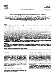
to a new arclength s. For the system under pressure, the tangent at each point (x(s), y(s)) on the segment makes an angle θ with the horizontal axis. Figure 1 shows the schematic of our cell wall system. The cell wall segment does not have any bending resistance, but has resistance to stretching. This stretching resistance is characterized by the Young’s modulus, E, of the cell wall segment. The stretching factor α is the ratio of the arclength under pressure compared to the zero pressure arc length s˜.

θ

(x(˜ s), y(˜ s))

s˜ = 0

s˜ = L

Figure 1: Schematic of a segment of the plant root cell wall. The segment is anchored at points (−b, 0) and (b, 0)

2.2

Expansion of the cell wall under turgor pressure

When the plant cell wall is subjected to a turgor pressure P , it expands. The expansion of the cell is governed by the Young-Laplace law P = T κ, where κ is the curvature of the cell wall. Under linear elasticity limits, the tension on the cell wall is T = E(α − 1). We develop a model for the final shape of the cell wall segment (x(s), y(s)), and the extension factor α, given a pressure P and a Young’s modulus E. The final state of the expanded cell wall segment is given by the following system of equations: dy dx = α cos θ, = α sin θ, d˜ s d˜ s T dθ ds P = , T = E(α − 1), α= , α d˜ s d˜ s where E is Young’s modulus, T is tension and α is the extension. The boundary conditions satisfied by these equations are x(˜ s = 0) = b,

x(˜ s = L) = −b,

y(˜ s = 0) = 0,

y(˜ s = L) = 0,

s(˜ s = 0) = 0.

It is convenient to solve this system of equations in a non-dimensional setting. We scale all length units by the arclength of the initial cell wall segment L which yields: x† =

x , L

y† =

y , L

s† = 2

s , L

s˜† =

s˜ , L

T† =

T . E

The dimensionless system of equations are: dx† = α cos θ, d˜ s† T † = α − 1,

dy † = α sin θ, d˜ s† ET † dθ ds† P = , α = †, αL d˜ s† d˜ s

with boundary conditions: x† (˜ s = 0) = b∗ ,

y † (˜ s = 0) = 0,

x† (˜ s = 1) = −b∗ ,

y † (˜ s = 1) = 0,

s† (˜ s† = 0) = 0,

where b∗ = b/L. Solving this set of equations yields: T† T† † sin θ + C, y = − cos θ + D, P∗ P∗ where the constants and other dependent parameters are given by the following equations:  ∗  T† P α C = 0, D = − cos , T † = α − 1. P 2T † x† =

The value of α is calculated by solving the following equation numerically:   P ∗ b∗ P ∗α = . sin 2(α − 1) (α − 1)

Figure 2: Final cell wall profiles for different pressures. Under no applied force from the AFM tip, the cell wall profiles all adopt sections of a circle. The symbol P on the figure refers to non-dimensional quantity P ∗ = P L/E. The cell wall is anchored at b = 1.

Figure 2 shows the profiles of the cell wall segment for a given initial segment length for different turgor pressures. We can clearly see that as the pressure increases, the arclength of the cell wall segment and the volume of the cell increase. What is the effect of the starting arclength L on the extension α? One would expect that for a given pressure P ∗ , as the length of the initial segment increases α would decrease. Figure 3 shows the extension α as a function of the initial arc length L for various pressures P ∗ . 3

Figure 3: The cell wall extension as a function of the initial starting lengths for different pressures. At a given pressure a longer cell wall segment expands less than a shorter segment. The symbol P on the figure refers to the non-dimensional quantity P ∗ = P L/E. The cell wall is anchored at b = 1.

2.3

Indentation of the cell wall under constant turgor pressure

In a typical AFM experiment (see Figure 4), a cantilever tip of cross-sectional area A, is brought into contact with the cell wall segment. A force is applied to indent the cell wall segment and the corresponding displacement of the cantilever tip is noted. We assume that the AFM probe is placed exactly at the center of the cell wall segment. Our aim here is to extend our model from the previous section to calculate the final shape of the cell wall segment given that a force F is acting at the point x† = 0 and y † = η.

Figure 4: A schematic of the AFM experiment with forcing at constant pressure conditions.

The system of equations we solve is the same set of equations presented in the previous section. The new boundary conditions are: x† (˜ s† = 0) = b∗ ,

x† (˜ s† = 1/2) = 0,

y † (˜ s† = 0) = 0,

F ∗ − P ∗ A∗ + 2T † sin θ1 = 0, 4

s† (˜ s† = 0) = 0,

Figure 5: The force versus displacement curve for the constant pressure forcing model.

where we use the following notation for convenience: θ(˜ s† = 0) = θ0 ,

θ(˜ s† = 1/2) = θ1 ,

y † (˜ s† = 1/2) = η.

Solving the system of equations using the new boundary conditions yields: x† =

T† sin θ + C, P∗

y† = −

T† cos θ + D, P∗

where P ∗α T† T† † + θ , T = α − 1, C = − sin θ , D = cos θ0 . 0 0 2T † P∗ P∗ The above set of equations can be reduced to the following two equations: θ1 =

P ∗ (2 sin θ1 + P ∗ A∗ − F ∗ ) , 2(P ∗ A∗ − F ∗ ) P ∗ A∗ − F ∗ (sin θ0 − sin θ0 ) , b∗ = 2P ∗ sin θ1 where the unknowns θ0 and θ1 are solved for numerically. θ1 − θ0 =

Figure 5 shows the force versus displacement curve for a given pressure P ∗ and initial length L. At a given pressure P ∗ , the indentation d, is a monotonically increasing function of the applied force F ∗ . This result is consistent with what is observed in typical AFM experiments. Figure 6 shows the final cell wall profiles for a given pressure under different applied forces on the AFM cantilever. We observe that as the applied force increases, the indentation increases, and the cell volume decreases to maintain the constant pressure inside the cell. Figure 7 shows the displacement of the AFM cantilever for a given applied force F ∗ as function of the internal pressure P ∗ . As the pressure inside the cell increases, the displacement or indentation due to the applied force decreases. These calculations suggest that our model is able to reproduce experimentally observed trends reasonably well. 5

Figure 6: Final cell profiles at equilibrium for applied forces. Note that the pressure inside the cell is constant, so the volume of the cell decreases as the applied force increases.

Figure 7: The displacement for a given applied force as a function of different cell pressures. For a given applied force, the displacement is smaller for higher cell pressures.

6

2.4

Indentation of the cell wall under constant cell volume

The AFM experiment can also be carried out at constant cell volume conditions, i.e. as we apply a force on the cell wall segment, the volume of the cell remains a constant, while the pressure inside the cell increases. The initial volume of the cell is calculated at a given initial pressure using the following expression  † Z θ1  † Z θ1 T T 0 y(θ)x (θ)dθ = V0 = cos θ + D cos θdθ P∗ P∗ θ0 θ0 2

=

2

T† T† T† (sin θ1 − sin θ0 ). (θ − θ ) − (sin 2θ − sin 2θ ) + D 1 0 1 0 P∗ 2P ∗ 2 4P ∗ 2

The additional constraint on the volume of the cell when a force is applied results in the following set of equations: x† =

T† sin θ + C, P∗

y† = −

T† sin(θ0 ) + C = b∗ , ∗ P −

T† cos(θ0 ) + D = 0, P∗

2

T† cos θ + D, P∗

T† sin(θ1 ) + C = 0, P∗ F ∗ − P ∗ A∗ + 2T † sin(θ1 ) = 0,

2

T† T† T† (θ − θ ) − (sin 2θ − sin 2θ ) + D (sin θ1 − sin θ0 ) = V0 , 1 0 1 0 P∗ 2P ∗ 2 4P ∗ 2 which are solved numerically.

Figure 8: Final cell profiles at different forcing conditions. Note that the pressure inside the cell is changing, and the volume of the cell is constant as the applied force increases.

7

Figure 8 shows the cell wall profiles under equilibrium for different forces. The volume of the cell is held constant and the pressure inside the cell increases. As the applied force increases, the indentation increases. The cell expands laterally to maintain a constant volume. This is consistent with physical expectations.

3

Conclusions

We have developed a simple 2D model for the outer wall of a plant root cell. This model is able to capture the effects of the turgor pressure on the final configuration/shape of the cell wall segment. The model was extended to calculate the final shape of the cell when it is subjected to a force from an AFM cantilever tip under constant pressure and constant volume conditions. The numerical solution of our model yields results which agree with expected experimental trends. The main limitation of our model is that it does not capture the presence of an inner cell membrane in plant cells. Typical AFM experiments are conducted on live roots. The response observed in these experiments will be from a system of pressurized cells which have common nodes. Our model explores the response of a single cell upon the application of a force by a cantilever beam. Future work on this project could be in the direction of developing models which calculates the mechanical properties of a network of pressurized cells. The future models can also incorporate flow of fluid in and out of the cell.

8