Introduction to Equivariant Cohomology in Algebraic Geometry Dave Anderson April 30, 2011 Abstract Introduced by Borel in the late 1950’s, equivariant cohomology encodes information about how the topology of a space interacts with a group action. Quite some time passed before algebraic geometers picked up on these ideas, but in the last twenty years, equivariant techniques have found many applications in enumerative geometry, Gromov-Witten theory, and the study of toric varieties and homogeneous spaces. In fact, many classical algebro-geometric notions, going back to the degeneracy locus formulas of Giambelli, are naturally statements about certain equivariant cohomology classes. These lectures survey some of the main features of equivariant cohomology at an introductory level. The first part is an overview, including basic definitions and examples. In the second lecture, I discuss one of the most useful aspects of the theory: the possibility of localizing at fixed points without losing information. The third lecture focuses on Grassmannians, and describes some recent “positivity” results about their equivariant cohomology rings.

Contents 1 Lecture 1: Overview 1.1 The Borel construction 1.2 Approximation spaces 1.3 Functorial properties . 1.4 Fiber bundles . . . . . 1.5 Two notions . . . . . .

. . . . .

. . . . .

. . . . .

. . . . . 1

. . . . .

. . . . .

. . . . .

. . . . .

. . . . .

. . . . .

. . . . .

. . . . .

. . . . .

. . . . .

. . . . .

. . . . .

. . . . .

. . . . .

. . . . .

. . . . .

. . . . .

. . . . .

2 3 4 5 7 8

2 Lecture Two: Localization 2.1 Restriction maps . . . . . . . . . . . . . . . . . . 2.2 Gysin maps . . . . . . . . . . . . . . . . . . . . . 2.3 First localization theorem . . . . . . . . . . . . . 2.4 Equivariant formality . . . . . . . . . . . . . . . . 2.5 Integration formula (Atiyah-Bott-Berline-Vergne) 2.6 Second localization theorem . . . . . . . . . . . . 3 Lecture 3: Grassmannians and Schubert 3.1 Pre-history: Degeneracy loci . . . . . . . 3.2 The basic structure of Grassmannians . . 3.3 Fixed points and weights . . . . . . . . . 3.4 Schubert classes in HT∗ X . . . . . . . . . 3.5 Double Schur functions . . . . . . . . . . 3.6 Positivity . . . . . . . . . . . . . . . . . 3.7 Other directions . . . . . . . . . . . . . .

1

. . . . . .

calculus . . . . . . . . . . . . . . . . . . . . . . . . . . . . . . . . . . . . . . . . . .

. . . . . . . . . . . . .

. . . . . . . . . . . . .

. . . . . . . . . . . . .

. . . . . . . . . . . . .

. . . . . . . . . . . . .

. . . . . .

9 9 10 12 12 13 14

. . . . . . .

15 15 17 18 19 19 22 24

Lecture 1: Overview

A general principle of mathematics holds that one should exploit symmetry to simplify a problem whenever possible. A common manifestation of symmetry is the action of a Lie group G on a topological space X — and when one is interested in understanding the cohomology ring H ∗ X, the equivariant cohomology HG∗ X is a way of exploiting this symmetry. Topologists have long been interested in a sort of converse problem: given some topological (or cohomological) information about X, what can one say about the kinds of group actions X admits? For example, must there be fixed points? How many? It was in this context that Borel originally defined what is now called equivariant cohomology, in his 1958–1959 seminar on transformation groups [Bo]. The goal of these lectures is to give a quick introduction to equivariant cohomology in the context of algebraic geometry. We will review the basic properties of HG∗ X and give some examples of applications. Ackowledgements. I learned much of what I know about equivariant cohomology from William Fulton, and the point of view presented here owes a debt to his lectures on the subject. I am grateful to the organizers of IMPANGA for arranging the excellent conference in which these lectures took 2

place. These notes were assembled with the help of Piotr Achinger, and I thank him especially for assistance in typing, researching literature, and clarifying many points in the exposition. I also thank the referee for valuable input and careful reading.

1.1

The Borel construction

Let G be a complex linear algebraic group, and let X be a complex algebraic variety with a left G-action. The construction Borel introduced in [Bo] goes as follows. Find a contractible space EG with a free (right) G-action. (Such spaces exist, and are universal in an appropriate homotopy category; we will see concrete examples soon.) Now form the quotient space EG ×G X := EG × X/(e · g, x) ∼ (e, g · x). Definition 1.1 The equivariant cohomology of X (with respect to G) is the (singular) cohomology of EG ×G X: HG∗ X := H ∗ (EG ×G X). (We always use singular cohomology with Z coefficients in these notes.) The idea behind the definition is that when X is a free G-space, we should have HG∗ X = H ∗ (G\X). To get to this situation, we replace X with a free G-space of the same homotopy type. From a modern point of view, this is essentially the same as taking the cohomology of the quotient stack [G\X] (see, e.g., [Be]). General facts about principal bundles ensure that this definition is independent of the choice of space EG; for instance, BG = EG/G is unique up to homotopy. When X is a point, EG ×G {pt} = BG usually has nontrivial topology, so HG∗ (pt) 6= Z! This is a key feature of equivariant cohomology, and HG∗ (pt) = H ∗ BG may be interpreted as the ring of characteristic classes for principal G-bundles. Other functorial properties are similar to ordinary cohomology, though. (In fact, HG∗ (−) is a generalized cohomology theory, on a category of reasonable topological spaces with a left G-action.) Example 1.2 Let G = C∗ . The space EG = C∞ r {0} is contractible, and G acts freely, so BG = EG/G = P∞ . We see that HC∗ ∗ (pt) = H ∗ P∞ ≃ Z[t], 3

where t = c1 (OP∞ (−1)) is the first Chern class of the tautological bundle.

1.2

Approximation spaces

The spaces EG and BG are typically infinite-dimensional, so they are not algebraic varieties. (This may partly account for the significant lag before equivariant techniques were picked up by algebraic geometers.) However, there are finite-dimensional, nonsingular algebraic varieties Em → Bm = Em /G which serve as “approximations” to EG → BG. This works because of the following lemma: Lemma 1.3 Suppose Em is any (connected) space with a free right G-action, and H iEm = 0 for 0 < i < k(m) (for some integer k(m)). Then for any X, there are natural isomorphisms H i (Em ×G X) ≃ H i(EG ×G X) =: HGi X, for i < k(m). Example 1.4 For G = C∗ , take Em = Cm r {0}, so Bm = Pm−1 . Since Em is homotopy-equivalent to the sphere S 2m−1 , it satisfies the conditions of the lemma, with k(m) = 2m − 1 in the above lemma. Note that k(m) → ∞ as m → ∞, so any given computation in HG∗ X can be done in H ∗ (Em ×G X), for m ≫ 0. We have Bm = Pm−1 , so Em → Bm is an intuitive choice for approximating EG → BG. Example 1.5 Similarly, for a torus T ≃ (C∗ )n , take Em = (Cm r {0})×n → (Pm−1 )×n = Bm . We see that HT∗ (pt) = HT∗ ((P∞ )n ) = Z[t1 , . . . , tn ], with ti = c1 (Oi(−1)). (Here Oi (−1)) is the pullback of O(−1) by projection on the ith factor.) The above example is part of a general fact: For linear algebraic groups G and H, one can always take E(G × H) = EG × EH. Indeed, G × H acts freely (on the right) on the contractible space EG × EH. ◦ Example 1.6 Consider G = GLn , and let Em := Mm×n be the set of full rank m × n matrices, for m > n. This variety is k(m)-connected, for k(m) =

4

◦ 2(m − n). Indeed, Mm×n is the complement of a closed algebraic set of codimension (m−1)(n−1) in Mm×n , and it is a general fact that πi (Cn rZ) = 0 for 0 < i ≤ 2d − 2 if Z is a Zariski closed subset of codimension d. See [Fu2, §A.4]. It follows that the maps

Em → Bm = Gr(n, Cm ) approximate EG → BG, in the sense of Lemma 1.3. We have HG∗ (pt) = Z[e1 , . . . , en ], where ei = ci (S) is the ith Chern class of the tautological bundle over the Grassmannian. Since any linear algebraic group G embeds in some GLn , the above example gives a construction of approximations Em that works for arbitrary G. Example 1.7 The partial flag manifold F l(1, 2, . . . , n; Cm ) parametrizes nested chains of subspaces E1 ⊂ E2 ⊂ · · · ⊂ En ⊂ Cm , where dim Ei = i. There is also an infinite version, topologized as the limit taking m → ∞. If B ⊂ GLn is the subgroup of upper-triangular matrices, we have ◦ Mm×n

Em =

?

?

Bm =F l(1, 2, . . . , n; Cm ), so BB is the partial (infinite) flag manifold F l(1, 2, . . . , n; C∞ ). Remark 1.8 The idea of approximating the infinite-dimensional spaces EG and BG by finite-dimensional ones can be found in the origins of equivariant cohomology [Bo, Remark XII.3.7]. More recently, approximations have been used by Totaro and Edidin-Graham to define equivariant Chow groups in algebraic geometry.

1.3

Functorial properties

Equivariant cohomology is functorial for equivariant maps: given a homoϕ f morphism G − → G′ and a map X − → X ′ such that f (g · x) = ϕ(g) · f (x), we get a pullback map f ∗ : HG∗ ′ X ′ → HG∗ X, 5

′

by constructing a natural map E ×G X → E′ ×G X ′ . There are also equivariant Chern classes and equivariant fundamental classes: • If E → X is an equivariant vector bundle, there are induced vector bundles Em ×G E → Em ×G X. Set G 2i 2i G cG i (E) = ci (Em × X) ∈ HG X = H (Em × X),

for m ≫ 0. • When X is a nonsingular variety, so is Em ×G X. If V ⊆ X is a Ginvariant subvariety of codimension d, then Em ×G V ⊆ Em ×G X has codimension d. We define [V ]G = [Em ×G V ] ∈ HG2d X = H 2d (Em ×G X), again for m ≫ 0. (Any subvariety of a nonsingular variety defines a class, using e.g. Borel-Moore homology.) G In fact, the Chern classes could be defined directly as cG i (E) = ci (EG × G E), but for [V ] one needs the approximation spaces. (Of course, one has to check that these definitions are compatible for different Em ’s.) In the special case X = pt, an equivariant vector bundle E is the same as a representation of G. Associated to any representation, then, we have 2i characteristic classes cG i (E) ∈ HG (pt).

Example 1.9 Let La = C be the representation of C∗ with the action z · v = za v where a is a fixed integer. Then ∗

Em ×C La ≃ OPm−1 (−a) ∗

as line bundles on Bm = Pm−1 , so cC1 (La ) = at ∈ Z[t]. (This also explains our choice of generator for HC∗ ∗ (pt) = Z[t]: we want t to correspond to the standard representation, L1 .)

6

Example 1.10 Let T = (C∗ )n act on E = Cn by the standard action. Then cTi (E) = ei (t1 , . . . , tn ) ∈ HT∗ (pt) = Z[t1 , . . . , tn ], where ei is the i-th elementary symmetric function. To see this, note that Em ×T E ≃ O1 (−1) ⊕ . . . ⊕ On (−1) as vector bundles on Bm = (Pm−1 )n . Problem 1.11 Let T be the maximal torus in GLn , and let E be an irreducible polynomial GLn -module. The above construction assigns to E its equivariant Chern classes cTi (E), which are symmetric polynomials in variables t1 , . . . , tn . What are these polynomials? Since they are symmetric polynomials, we can write X cTi (E) = aλ sλ (t), λ

where sλ are the Schur polynomials (which are defined in §3 below). A theorem of Fulton and Lazarsfeld implies that the integers aλ are in fact nonnegative, as was observed by Pragacz in [P, Corollary 7.2]. This provides further motivation for the problem: we are asking for a combinatorial interpretation of the coefficients aλ .

1.4

Fiber bundles

The formation of E×G X is really an operation of forming a fiber bundle with ρ ρ fiber X. The map X − → pt becomes E ×G X − → B (via the first projection); ordinary cohomology H ∗ X is an algebra over H ∗ (pt) = Z (i.e., a ring), while HG∗ X is an algebra overHG∗ (pt); and one can generally think of equivariant geometry as the geometry of bundles. From this point of view, many statements about equivariant cohomology are essentially equivalent to things that have been known to algebraic geometers for some time—for instance, the Kempf-Laksov formula for degeneracy loci is the same as a “Giambelli” formula in HT∗ Gr(k, n). Example 1.12 (Equivariant cohomology of projective space) Let T = (C∗ )n act on Cn in the usual way, defining an action on Pn−1 = P(Cn ). This makes OP(Cn ) (1) a T -equivariant line bundle. Write ζ = cT1 (OPn−1 (1)). 7

Claim 1 We have HT∗ Pn−1 ≃ Z[t1 , . . . , tn ][ζ]/(ζ n + e1 (t)ζ n−1 + · · · + en (t)) Q = Z[t1 , . . . , tn ][ζ]/( ni=1 (ζ + ti )). Proof. Pass from the vector space Cn to the vector bundle E = Em ×T Cn on Bm . We have Em ×T Pn−1 ≃ P(E)

Em ×T OPn−1 (1) ≃ OP(E) (1),

and

all over Bm . The claim follows from the well-known presentation of H ∗ P(E) over H ∗ B, since ei (t) = cTi (Cn ) = ci (E)

ζ = cT1 (OPn−1 (1)) = c1 (OP(E) (1)),

and

as in Example 1.10.

1.5

Two notions

There are two general notions about equivariant cohomology to have in mind, especially when G is a torus. The first notion is that equivariant cohomology determines ordinary cohomology. From the fiber bundle picture, with the commutative diagram X

⊂

-

E ×G X ?

?

pt ⊂

-

B,

HG∗ X is an algebra over HG∗ (pt), and restricting to a fiber gives a canonical map HG∗ X → H ∗ X, compatible with HG∗ (pt) → H ∗ (pt) = Z. In nice situations, we will have: HG∗ X → H ∗ X is surjective, with kernel generated by the kernel of HG∗ (pt) → Z. The second notion is that equivariant cohomology is determined by information at the fixed locus. By functoriality, the inclusion of the fixed locus ι : X G ֒→ X gives a restriction (or “localization”) map ι∗ : HG∗ X → HG∗ X G . In nice situations, we have: 8

ι∗ : HG∗ X → HG∗ X G is injective. Example 1.13 Both of these notions can fail, even when G is a torus. For example, take G = X = C∗ , where G acts on itself via left multiplication. One the one hand, ∗

HC1 ∗ (C∗ ) = H 1 ((C∞ r {0}) ×C C∗ ) = H 1 (C∞ r {0}) = 0, but on the other hand, H 1 (C∗ ) = H 1 (S 1 ) = Z, so the first notion fails. Since the action has no fixed points, the second cannot hold, either. However, we will see that the “nice” situations, where both notions do hold, include many interesting cases. When the second notion holds, it provides one of the most powerful techniques in equivariant theory. To get an idea of this, suppose X has finitely many fixed points; one would never expect an injective restriction map ι∗ in ordinary cohomology, by degree reasons! Yet in many situations, all information about HT∗ X is contained in the fixed locus. This will be the topic of the next lecture.

2

Lecture Two: Localization

From now on, we will consider only tori: G = T ≃ (C∗ )n . Since it comes up often, it is convenient introduce notation for the equivariant cohomology of a point: Λ = ΛT = HT∗ (pt) ≃ Z[t1 , . . . , tn ].

2.1

Restriction maps

If X is a T -space and p ∈ X is a fixed point, then the inclusion ιp : {p} → X is equivariant, so it induces a map on equivariant cohomology ι∗p : HT∗ X → XT∗ ({p}) = Λ. Example 2.1 Let E be an equivariant vector bundle of rank r on X, with Ep the fiber at p. Then ι∗p (cTi (E)) = cTi (Ep ), as usual. Now Ep is just a representation of T , say with weights (characters) χ1 , . . . , χr . That is, Ep ≃ Cr , and t · (v1 , . . . , vr ) = (χ1 (t)v1 , . . . , χr (t)vr ) for homomorphisms 9

χi : T → C∗ . So cTi (Ep ) = ei (χ1 , . . . , χr ) is the ith elementary symmetric polynomial in the χ’s. In particular, the top Chern class goes to the product of the weights of Ep : ι∗p (cr (E)) = χ1 · · · χr . Example 2.2 Consider X = Pn−1 with the standard action of T = (C∗ )n , so (t1 , . . . , tn ) · [x1 , . . . , xn ] = [t1 x1 , . . . , tn xn ]. The fixed points of this action are the points pi = [0, . . . , 0, 1, 0, . . . , 0] for i = 1, . . . , n. | {z } i

The fiber of the tautological line bundle O(−1) at pi is the coordinate line C · εi , so T acts on O(−1)pi by the character ti , and on O(1)pi by −ti . In the notation of Example 1.9, O(−1)pi ≃ Lti and O(1)pi ≃ L−ti . Setting ζ = cT1 (O(1)), we see that ι∗pi ζ = −ti . Exercise 2.3 Show that the map of Λ-algebras Λ[ζ]/

n Y

(ζ + ti )

-

i=1

ζ

-

Λ⊕n

(−t1 , . . . , −tn ) ι∗

is injective. (By Examples 1.12 and 2.2, this is the restriction map HT∗ Pn−1 − → L ∗ n−1 T ∗ HT (P ) = HT (pi ).)

2.2

Gysin maps

For certain kinds of (proper) maps f : Y → X, there are Gysin pushforwards f∗ : HT∗ Y → HT∗+2d X, as in ordinary cohomology. Here d = dim X − dim Y . We’ll use two cases, always assuming X and Y are nonsingular varieties. 1. Closed embeddings. If ι : Y ֒→ X is a T -invariant closed embedding of codimension d, we have ι∗ : HT∗ Y → HT∗+2d X. This satisfies: 10

(a) ι∗ (1) = ι∗ [Y ]T = [Y ]T is the fundamental class of Y in HT2d X. (b) (self-intersection) ι∗ ι∗ (α) = cTd (NY /X ) · α, where NY /X is the normal bundle. 2. Integral. For a complete (compact) nonsingular variety X of dimension n, the map ρ : X → pt gives ρ∗ : HT∗ X → HT∗−2n (pt). Example 2.4 Let T act on P1 with weights χ1 and χ2 , so t · [x1 , x2 ] = [χ1 (t)x1 , χ2 (t)x2 ]). Let p1 = [1, 0], p2 = [0, 1] as before. Setting χ = χ2 − χ1 , the tangent space Tp1 P1 has weight χ: t · [1, a] = [χ1 (t), χ2 (t)a] = [1, χ(t)a]. Similarly, Tp2 P1 has weight −χ. So ι∗p1 [p1 ]T = cT1 (Tp1 P1 ) = χ, and ιp2 [p2 ]T = −χ. (And the other restrictions are zero, of course.) From Example 2.2, we know ι∗p1 ζ = −χ1 = χ − χ2 and ι∗p1 ζ = −χ2 = −χ − χ1 , so [p1 ]T = ζ + χ2

and

[p2 ]T = ζ + χ1

in HT∗ P1 . Exercise 2.5 More generally, show that if T acts on Pn−1 with weights χ1 , . . . , χn , then Y [pi ]T = (ζ + χj ) j6=i

in HT∗ Pn−1 . Example 2.6 If p ∈ Y ⊆ X, with X nonsingular, and p a nonsingular point on the (possibly singular) subvariety Y , then ι∗p [Y ]T = cTd (Np ) =

d Y

χi

i=1

in Λ = HT∗ (p), where the χi are the weights on the normal space Np to Y at p.

11

2.3

First localization theorem

Assume that X is a nonsingular variety, with finitely many fixed points. Consider the sequence of maps M M ι∗ ι∗ Λ = HT∗ X T − → HT∗ X − → HT∗ X T = Λ. p∈X T

p∈X T

L L The composite map ι∗ ι∗ : Λ→ Λ is diagonal, and is multiplication by T cn (Tp X) on the summand corresponding to p. Theorem 2.7 Let S ⊆ Λ be a multiplicative set containing the element Y c := cTn (Tp X). p∈X T

(a) The map S −1 ι∗ : S −1 HT∗ X → S −1 HT∗ X T

(∗)

is surjective, and the cokernel of ι∗ is annihilated by c. (b) Assume in addition that HT∗ X is a free Λ-module of rank at most #X T . Then the rank is equal to #X T , and the above map (*) is an isomorphism. Proof. For (a), it suffices to show that the composite map S −1 (ι∗ ◦ι∗ ) = S −1 ι∗ ◦ S −1 ι∗ is surjective. This in turn follows from the fact that the determinant Y det(ι∗ ◦ ι∗ ) = cTn (Tp X) = c p

becomes invertible after localization. For (b), surjectivity of S −1 ι∗ implies rank HT∗ X ≥ #X T , and hence equality. Finally, since S −1 Λ is noetherian, a surjective map of finite free modules of the same rank is an isomorphism.

2.4

Equivariant formality

The question arises of how to verify the hypotheses of Theorem 2.7. To this end, we consider the following condition on a T -variety X:

12

(EF) HT∗ X is a free Λ-module, and has a Λ-basis that restricts to a Z-basis for H ∗ X. Using the Leray-Hirsch theorem, this amounts to degeneration of the LeraySerre spectral sequence of the fibration E ×T X → B. A space satisfying the condition (EF) is often called equivariantly formal, a usage introduced in [GKM]. One common situation in which this condition holds is when X is a nonsingular projective variety, with X T finite. In this case, the Bialynicki-Birula decomposition yields a collection of T -invariant subvarieties, one for each fixed point, whose classes form a Z-basis for H ∗ X. The corresponding equivariant classes form a Λ-basis for HT∗ X restricting to the one for H ∗ X, so (EF) holds. Moreover, since the basis is indexed by fixed points, HT∗ X is a free Λ-module of the correct rank, and assertion (b) of Theorem 2.7 also holds. Corollary 2.8 The “two notions” from §1.5 hold for a nonsingular projective T -variety with finitely many fixed points: HT∗ X ։ H ∗ X

and

HT∗ X ֒→ HT∗ X T .

Remark 2.9 Condition (EF) is not strictly necessary to have an injective localization map S −1 HT∗ X → S −1 HT∗ X T . In fact, if one takes S = Λ r {0}, no hypotheses at all are needed on X: this map is always an isomorphism (though the rings may become zero); see [H, §IV.1]. On the other hand, this phenomenon is peculiar to torus actions. For example, the group B of upper-triangular matrices acts on Pn−1 with only one fixed point. However, since B admits a deformation retract onto the diagonal torus T , the ring HB∗ Pn−1 = HT∗ Pn−1 is a free module over ΛB = ΛT . There can be no injective map to HB∗ (Pn−1 )B = HB∗ (pt) = Λ, even after localizing. (The difference is that HB∗ (X r X B ) is not necessarily a torsion ΛB -module when B is not a torus.)

2.5

Integration formula (Atiyah-Bott-Berline-Vergne)

Theorem 2.10 Let X be a compact nonsingular variety of dimension n, with finitely many T -fixed points. Then X ι∗p α ρ∗ α = cTn Tp X T p∈X

for all α ∈

HT∗ X. 13

Proof. Since ι∗ : S −1 HT∗ X T → HT∗ X is surjective, it is enough to assume α = (ιp )∗ β, for some β ∈ HT∗ (p) = Λ. Then the LHS of the displayed (ιp )∗

ρ∗

equation is ρ∗ α = ρ∗ (ιp )∗ β = β. (The composition HT∗ (p) −−→ HT∗ X −→ Λ is an isomorphism.) The RHS is X ι∗q (ιp )∗ β ι∗p (ιp )∗ β = T = β, cTn Tq X cn Tp X T

q∈X

using the self-intersection formula for the last equality. Example 2.11 Take X = Pn−1 , with the standard action of T via character t1 , . . . , tn , and let ζ = cT1 (O(1)). Then one computes  2k−2(n−1) 0 if k < n − 1, by degree: HT (pt) = 0; k ρ∗ (ζ ) = 1 if k = n − 1, by ordinary cohomology. On the other hand, using the localization formula, we obtain k

ρ∗ (ζ ) =

n X i=1

(−ti )k , j6=i (tj − ti )

Q

yielding a nontrivial algebraic identity! Remark 2.12 Ellingsrud and Strømme [ES] used this technique, with the aid of computers, to find the answers to many difficult enumerative problems, e.g., the number of twisted cubics on a Calabi-Yau three-fold. As an illustrative exercise, one could compute the number of lines passing through to four given lines in P3 . (Use localization for the action of T ≃ (C∗ )4 on the Grassmannian Gr(2, 4).) A more challenging problem is to compute number of conics tangent to five given conics in P2 , via localization for the action of T ≃ (C∗ )2 on the space of complete conics; see, e.g., [Br2, p. 15].

2.6

Second localization theorem

A remarkable feature of equivariant cohomology is that one can often characterize the image of the restriction map ι∗ : HT∗ X → HT∗ X T , realizing HT∗ X as a subring of a direct sum of polynomial rings. To state a basic version of the theorem, we use the following hypothesis. For characters χ and χ′ appearing as weights of Tp X, for p ∈ X T , assume: 14

(*). if χ and χ′ occur in the same Tp X they are relatively prime in Λ. Condition (*) implies that for each p ∈ X T and each χ occurring as a weight for Tp X, there exists a unique T -invariant curve E = Eχ,p ≃ P1 through p, with Tp E ≃ Lχ . By Example 2.4, E T = {p, q}, and Tq E has character −χ. Theorem 2.13 Let X be a nonsingular variety with X T finite, and assume (*) holds. Then an element M (up ) ∈ Λ = HT∗ X T p∈X T

lies in ι∗ HT∗ X if and only if, for all E = Eχ,p = E−χ,q , the difference up − uq is divisible by χ. As with the other localization theorems, the idea of the proof is to use the Gysin map and self-intersection formula, this time applied to the compositions HT∗ X T → HT∗ X χ → HT∗ X → HT X χ → HT∗ X T , where X χ is a union of invariant curves Eχ for a fixed character χ. For a detailed proof, see [Fu2, §5]. The theorem is originally due to Chang and Skjelbred [CS]. It was more recently popularized in an algebraic geometry context by Goresky-KottwitzMacPherson [GKM]. The utility of this characterization is that it makes HT∗ X a combinatorial object: the ring can be computed from the data of a graph whose vertices are the fixed points X T and whose edges are the invariant curves E = Eχ,p = E−χ,q .

3 3.1

Lecture 3: Grassmannians and Schubert calculus Pre-history: Degeneracy loci

Let X be a Cohen-Macaulay variety, and let E be a rank n vector bundle on X, admitting a filtration 0 = E0 ⊂ E1 ⊂ . . . ⊂ En = E,

15

where

rank Ei = i.

Let F be a rank r vector bundle, and let ϕ : E → F be a surjective morphism. Given a partition λ = (r ≥ λ1 ≥ λ2 ≥ . . . ≥ λn−r ≥ 0), the associated degeneracy locus is defined as ϕ(x)

Dλ (ϕ) = {x ∈ X | rank(Er−λi +i (x) −−→ F (x)) ≤ r−λi for 1 ≤ i ≤ n−r} ⊆ X. Since these schemes appear frequently in algebraic geometry, it is very useful to have a formula for their cohomology classes. Such a formula was given by Kempf and Laksov [KL], and independently by Lascoux [L]: Theorem 3.1 (Kempf-Laksov) Set k = n − r. When codim Dλ = |λ| := P λi , we have [Dλ ] = ∆λ (c(F − E)) := det(cλi +j−i (i)) cλ1 (1) cλ1 +1 (1) · · · cλ1 +k−1 (1) .. cλ2 (2) . cλ2 −1 (2) = . .. . .. .. . c ··· ··· cλk (k) λk −k+1 (k)

in H ∗ X, where cp (i) = cp (F − Er−λi +i ).



Here the notation c(A − B) = c(A)/c(B) means the formal series expansion of (1 + c1 (A) + c2 (A) + · · · )/(1 + c1 (B) + c2 (B) + · · · ), and cp is the degree p term. The proof of this theorem starts with a reduction to the Grassmannian bundle π : Gr(k, E) → X. Since ϕ is surjective, the subbundle K = ker(ϕ) ⊆ E has rank k, and it defines a section σ : X → Gr(k, E) such that σ ∗ S = K. (Here S ⊆ π ∗ E is the tautological rank k bundle on Gr(k, E).) In fact, the theorem is equivalent to a formula in equivariant cohomology. The universal base for rank n bundles with filtration is BB; see Example 1.7. Consider the following diagram: Gr(k, E) - Gr(k, E ) g π ? f - ? X BB. Writing E1 ⊂ E2 ⊂ · · · ⊂ En = E for the tautological sequence on BB = F l(1, 2, . . . , n; C∞ ), the map f is defined by Ei = f ∗ Ei for 1 ≤ i ≤ n. The 16

map g is defined by F = g ∗ F , where E → F is the universal quotient on Gr(k, E ). Now a formula for Dλ in H ∗ X can be pulled back from a universal formula for a corresponding locus Ωλ in H ∗ Gr(k, E ) = HB∗ Gr(k, Cn ) = HT∗ Gr(k, Cn ). We will see how such a formula can be deduced combinatorially, using equivariant localization. Remark 3.2 Some extra care must be taken to ensure that the bundles Ei and F are pulled back from the algebraic approximations Bm ; see, e.g., [G1, p. 486].

3.2

The basic structure of Grassmannians

The Grassmannian X = Gr(k, Cn ) is the space of k-dimensional linear subspaces in Cn and can be identified with the quotient ◦ Mn×k /GLk

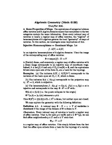
of the set of full-rank n by k matrices by the action of GLk by right multiplication. The groups T ≃ (C∗ )n ⊂ B ⊂ GLn act on X by left multiplication. For any k-element subset I ⊂ {1, . . . , n}, we denote by UI the set of all k-dimensional linear subspaces of Cn whose projection on the subspace spanned by the vectors {ei | i ∈ I}, where {e1 , . . . , en } is the standard basis for Cn . It follows that UI ≃ Ck(n−k) and UI is open in X. Indeed, UI can be identified with the set of k × (n − k) matrices M whose square submatrix on rows I is equal to the k × k identity matrix. For I = {2, 4, 5}, we have   ∗ ∗ ∗        1 0 0         ∗ ∗ ∗    . UI =  0 1 0            0 0 1        ∗ ∗ ∗

In particular, dim X = k(n − k). The topology of Gr(k, Cn ) is easily studied by means of the decomposition into Schubert cells: Each point p ∈ X has an “echelon” form, that is, it can

17

be represented by a full rank n × k  ∗  1   ∗   0   0 0

matrix such as  ∗ ∗ 0 0   ∗ 0  . 1 0   0 1  0 0

We denote the set of rows with 1’s by I (so in the example above, I = {2, 4, 5}) and call it the pivot of the corresponding subspace. For any k-element subset I ⊂ {1, . . . , n}, the set Ω◦I of points with pivot I forms a cell, isomorphic to an affine space of dimension equal to the number of stars in the matrix. These are called Schubert cells, and they give a cell decomposition of X. Summarizing, we have open

closed

Ω◦I ֒→ UI ֒→ X. Note that Ω◦I and UI are T -stable.

3.3

Fixed points and weights

Let pI ∈ UI be the origin, that is, the point corresponding to the subspace spanned by {ei | i ∈ I}. Working with matrix representatives, the following basic facts are easy to prove: sees that • The T -fixed
points in X are precisely the points pI . In particular, #X T = nk . • The weights of T on TpI X = TpI UI ≃ UI are {tj − ti | i ∈ I, j ∈ / I}. • The weights of T on TpI Ω◦I are {tj − ti | i ∈ I, j ∈ / I, i > j}. • The weights of T on NΩI /X,pI are {tj − ti | i ∈ I, j ∈ / I, i < j}. Example 3.3 With I  0 0  1 0   0 a z·  0 1   0 0 0 0

= {2, 4, 5}, one sees that t4 − t3 is a     0 0 0 0 0 0  z2 0 0   1 0 0      z3    0   =  0 z3 a 0  ≡  0 z4 a    0    0 z4 0   0 1 1   0 0 z5   0 0 0 0 0 0 0 0 18

weight on TpI Ω◦I :  0 0   0  . 0   1  0

The other weights can be determined in a similar manner.

3.4

Schubert classes in HT∗ X

The closure ΩI := Ω◦I of a Schubert cell is called a Schubert variety. It is a disjoint union of all Schubert cells Ω◦J for J ≤ I with respect to the Bruhat order : J ≤ I iff j1 ≤ i1 , j2 ≤ i2 , . . . , jk ≤ ik . Since the Schubert cells have even (real) dimension, it follows that the classes of their closures form bases for H ∗ X and HT∗ X: M M Z · [ΩI ] and HT∗ X = Λ · [ΩI ]T . H ∗X = I

I

In particular, HT∗ X is free over Λ, of the correct rank, so the localization theorems apply. Let us record two key properties of Schubert classes. From the description of weights, and from Example 2.6, it follows that Y ι∗pI [ΩI ]T = (tj − ti ). (1) i∈I j ∈I / i