Federal Reserve Bank of Dallas Globalization and Monetary Policy Institute Working Paper No. 181 http://www.dallasfed.org/assets/documents/institute/wpapers/2014/0181.pdf

International Capital Flows and the Boom-Bust Cycle in Spain * Jan In’t Veld DG-ECFIN, EU Commission Beatrice Pataracchia JRC, EU Commission

Robert Kollmann ECARES, Université Libre de Bruxelles and CEPR

Werner Roeger DG-ECFIN, EU Commission

Marco Ratto JRC, EU Commission

May 2014 Abstract We study the joint dynamics of foreign capital flows and real activity during the recent boom- bust cycle of the Spanish economy, using a three-country New Keynesian model with credit- constrained households and firms, a construction sector and a government. We estimate the model using 1995Q1-2013Q2 data for Spain, the rest of the Euro Area (REA) and the rest of the world. We show that falling risk premia on Spanish housing and nonresidential capital, a loosening of collateral constraints for Spanish households and firms, as well as a fall in the interest rate spread between Spain and the REA fuelled the Spanish output boom and the persistent rise in foreign capital flows to Spain, before the global financial crisis. During and after the global financial crisis, falling house prices, and a tightening of collateral constraints for Spanish borrowers contributed to a sharp reduction in capital inflows, and to the persistent slump in Spanish real activity. The credit crunch was especially pronounced for Spanish households; firm credit constraints tightened later and more gradually, and contributed much less to the slump. JEL codes: C11, E21, E32, E62

*

Jan in’t Veld, DG-ECFIN, EU Commission, [email protected]. Robert Kollmann, European Centre for Advanced Research in Economics and Statistics (ECARES), CP 114, Université Libre de Bruxelles, 50 Av. Franklin Roosevelt, B-1050 Brussels, Belgium. 32-2-650-4474. [email protected]. www.robertkollmann.com. Beatrice Pataracchia, JRC, EU Commission. [email protected]. Marco Ratto, JRC, EU Commission, [email protected]. Werner Roeger, DG-ECFIN, EU Commission, [email protected]. We thank Menzie Chinn and Massimiliano Pisani for advice. Useful suggestions were also received from Francisco de Castro, Massimo Suardi and from conference participants at the European Commission. Research support from Jukka Heikkonen is gratefully acknowledged. The views in this paper are those of the authors and do not necessarily reflect the views of the European Commission, the Federal Reserve Bank of Dallas or the Federal Reserve System.

1. Introduction After the launch of the Euro in 1999, Greece, Ireland, Portugal, Spain, and other countries in the EU periphery ran sizable current account deficits. This was often accompanied by output and construction booms in these countries, and by inflation rates above the Euro Area average. In the wake of the global financial crisis (2008-09), private capital flows to the periphery countries fell sharply, and a strong contraction in real activity and asset prices occurred.1 This paper provides a quantitative analysis of the joint dynamics of the trade balance and real activity in Spain, the largest of the Euro Area countries that received sizable capital inflows after the creation of the Euro, and then experienced a sudden stop. We do so using a three-country New Keynesian Dynamic Stochastic General Equilibrium (DSGE) model consisting of Spain, an aggregate of the Rest of the Euro Area (REA) and an aggregate of the rest of the world (ROW).2 We estimate the model using quarterly data for Spain, the REA and the ROW during the period 1995Q1-2013Q2. The Spanish block of the model has a rich structure that allows us to capture the key features of the Spanish boom-bust cycle. In particular, we assume a construction sector and a government; Spanish households and nonfinancial firms face collateral constraints (à la Kiyotaki and Moore (1997)). The model assumes nominal price and wage rigidities, as well as demand and supply shocks in goods, labor and asset markets. We use the model as a laboratory for quantifying the key drivers and transmission mechanisms that have affected the Spanish economy since 1995. The creation of the Euro eliminated intra-Euro Area currency risk and led to a convergence of Spanish interest rates to the lower interest rates in the REA. Two other factors that may have caused the boom in the Spanish economy were loosening credit conditions, and asset bubbles. Our estimates suggest that these three factors all fuelled a sharp rise in Spanish investment and house prices, and increased the fragility of the balance sheets of Spanish households and non-financial firms. During the global financial crisis, a fall in Spanish asset prices, and a tightening of collateral constraints, led to a sharp improvement in the Spanish trade balance and current account, and to a persistent fall in Spanish residential and nonresidential investment and output. The credit crunch was especially pronounced for Spanish households. Firm credit constraints tightened later and more gradually, and contributed much less to the slump.

1

See Hale and Obstfeld (2014) and Hobza and Zeugner (2014) for detailed overviews of capital flows in the European Union. 2 Throughout this paper, the term ‘Euro Area’ (EA) refers to the 17 countries that were members of the Euro Area in 2013. REA is the EA less Spain. 2

Our analysis highlights the key role of domestic asset bubbles (explained in the model by exogenous asset risk-premium shocks) for the Spanish boom-bust cycle. In related analyses (not based on quantitative models), Reis (2013) and Fernández-Villaverde et al. (2013) argue that the pre-crisis boom in Spain (and in other Euro Area periphery countries) was largely driven by the convergence of Spanish interest rates to REA rates. While our model estimates show that interest rate convergence mattered for Spain, we find that asset bubbles and the loosening of credit constraints for households and firms had a more pronounced role. In the aftermath of the global financial crisis, Spanish real house prices continued to fall, while equity prices stabilized after 2010. Household deleveraging during this period has been achieved through a fall in residential investment, while aggregate consumption as a share of GDP has remained comparatively stable. The tightening of firm credit constraints during the aftermath of the global crisis was partly off-set by a fall in the risk-premium on production capital. During the Spanish sovereign debt crisis, foreign private lending to Spain fell sharply—however, credit to Spanish households and non-financial firms was stabilized through the massive substitution of foreign private lending by central bank lending. The recovery of the world economy and increased productivity growth in Spain also contributed to the Spanish trade balance improvement, in the aftermath of the global financial crisis. Our paper contributes to the literature that quantifies financial shocks before and during the financial crisis. By analyzing a wider range of financial shocks (interest rate spreads, risk premia on housing and production capital, shocks to collateral constraints of households and firms) in an estimated open economy model, we can more precisely identify the timing and relative importance of individual financial shocks. In related studies, Justiniano et al. (2013, 2014) quantify the effect of household leveraging and deleveraging in the US economy, using a calibrated DSGE model.3 These authors emphasize the importance of distinguishing changes in credit due to shocks to loan-to-value (LTV) ratios from changes in credit induced by asset price fluctuations. Justiniano et al. argue that shocks to LTV ratios per se cannot explain the recent boom-bust cycle of US house prices. The results in the paper here (for Spain) are consistent with this conclusion. We show that the boom-bust cycle in asset prices and real activity is better explained by shocks to risk premia on housing and other capital assets. Different from Justiniano et al., the model here also allows for credit constraints

3

See also Eggertsson and Krugman (2012) and Guerrieri and Lorenzoni (2012) for theoretical analyses of the macroeconomic effects of a credit constraint tightening, in a closed economy. 3

for firms. The fact that within the Euro Area monetary policy only very partially targets the Spanish economy is an additional amplifying mechanism, in our model. Several recent empirical studies have also highlighted the role of housing and credit markets for the dynamics of the current account (e.g., Aizenman and Jinjarak (2013), Chinn et al. (2013), Obstfeld and Rogoff (2010)). The paper here analyzes that role using an estimated DSGE model. The present paper is also related to a literature that analyzes current account dynamics using DSGE models (e.g., Kollmann (1998, 2001), Erceg et al. (2006), Gomes et al. (2012), Hürtgen and Rühmkorf (2014)); by contrast to the paper here, that literature has typically used calibrated models (not estimated), and it has abstracted from housing markets and the key financial frictions and shocks considered in the present model. The economic events in Spain (and other European periphery countries) during the past 15 years are reminiscent of the boom-bust cycles characterized by capital inflows and sudden stops experienced by many economies in Latin America and Asia during the 20 th century; see Adalet and Eichengreen (2007) for an empirical overview. The theoretical literature on sudden stops uses highly stylized models; see, e.g., Calvo (1998). By contrast, the present paper analyzes a boom-bust cycle linked to international capital in- and outflows, using a fully-fledged estimated DSGE model. Economic theory suggests that a country’s external balance reflects domestic and foreign macroeconomic and financial shocks, and the structural features of the domestic and foreign economies. This underscores the importance of analyzing the external balance using an estimated state-of-the art dynamic general equilibrium model that captures the relevant shocks, and their transmission to the macroeconomy. The paper here builds on in’t Veld et al. (2012) who analyzed the Spanish business cycle using a small open economy model that assumes a housing sector and credit constrained household, while firms are not credit constrained. As the creation of the Euro has increased financial integration in Europe, the present paper assumes that Spanish households too can borrow internationally, subject to collateral constraints (we also assume that firms are financially constrained, as mentioned above). In addition, the paper here uses a three-country model that allows to better capture the key external shocks affecting Spain. Sect. 2 describes the Spanish macroeconomy since the 1990s. Sect. 3 presents our model. Sect. 4 and 5 discuss the econometric approach and present the empirical results.

2. Dynamics of the Spanish macroeconomy For most of the decade up to 2007, GDP growth in Spain exceeded growth in the REA (see Fig. 1.a). But the global crisis hit Spain severely, with the year-on-year GDP growth rate falling to -4.6% in 2009Q2. Spain experienced a weaker recovery in 2010-11 than the REA, 4

and entered into a second-dip recession in 2012. During the Spanish boom years, the growth of domestic demand exceeded GDP growth. In particular, the ratios of residential and nonresidential investment to GDP both grew by about 5 percentage points until the financial crisis, and then experienced a downward correction of the same amount (Fig. 1.b). By contrast the Spanish consumption-to-GDP ratio rose only mildly until the crisis, and then fell slightly. The Spanish trade balance/GDP ratio showed a large and persistent decline between the end of the 1990s and 2007 (reaching -6% in 2007). The trade balance then rose rapidly in 2008, was stable at about -2% until the end of 2010, and then started to improve again, reaching positive values in 2012-13 (Fig. 1.c). These trade balance fluctuations were largely driven by the sizable rise in Spanish investment during the boom, and the subsequent contraction of investment. The Spanish saving rate shows positive co-movement with the investment rate (rising during the boom, and falling after the crisis), but fluctuated much less (Fig.1.d). 4 The Spanish balance of net foreign income and transfers has become gradually more negative during the sample period (reflecting Spain’s growing net foreign liabilities). Spain’s current account balance has, thus, been smaller than the trade balance; however, the fluctuations of the current account are dominated by the dynamics of the trade balance (Fig. 1.c). The external deficits prior to the crisis led to a strong rise in Spain’s net foreign liabilities--from around 20% of GDP in the mid-1990s to more than 90% of GDP by 2009 (Fig. 1.e). The rise in the trade balance since the global crisis has stabilized Spain’s net foreign liabilities. Flow of funds data show that the sharp increase in Spanish net foreign liabilities before the crisis was largely driven by a rise in the net foreign liabilities of the Spanish corporate sector, especially of banks; the net foreign liabilities of the financial sector reached 50% of annual GDP in 2008Q1, and stayed at about that value until 2011Q2. After 2011Q2, foreign investors sharply reduced their lending to Spanish commercial banks. Those banks then borrowed from the Bank of Spain to repay foreign liabilities, and the Bank of Spain borrowed abroad, essentially from the ECB (‘target balances’). This official financing stabilized aggregate Spanish net foreign liabilities (see Fig. 1.e). Spanish inflation (GDP deflator) averaged 3.5% p.a. in 1995-2007, and thus markedly exceeded the EA average (2.0%); the financial crisis led to a fall in inflation, below average EA inflation (Fig. 1.g). Thus, the Spanish real effective exchange rate appreciated steadily during the boom period, and depreciated during and after the bust. High inflation also implied that Spain had markedly lower real interest rates than the REA, prior to the financial crisis.

4

The ‘saving’ rate in Fig. 1.d is s≡(GDP-private consumption-government consumption)/ GDP; thus NX/GDP=s-investment/GDP; NX: net exports (all variables are in nominal terms). 5

Real house prices (relative to the GDP deflator) rose by 80% between 2001 and 2008, and have been falling steadily since then; by 2012 real house prices had fallen back to their 2003 values. This suggests that a housing bubble developed in Spain, before the crisis. Before the launch of the Euro (1.1.1999), Spanish nominal interest rates were markedly higher than rates in the REA. The creation of the Euro led to a convergence of Spanish nominal rates to Euro Area rates. The average Spanish government interest rate (interest payments/sovereign debt stock) fell from around 9% in the late 1990s to below 4% by 2010, but has since risen again (Fig. 1.f). While Spanish households’ borrowing costs have moved in line with the ECB policy rate, typically around 200 bps higher, there has been a marked increase in interest rates for non-financial firms in recent years, despite falling policy rates. Before the crisis, Spain’s public finances were in better health than the Euro Area average. Spanish government balances improved markedly between the mid-1990s and the mid-2000s (Fig. 1.c). The crisis then led to a sharp deterioration of public finances. [INSERT FIGURE 1 ABOUT HERE]

3. Model description We consider a three-country world consisting of Spain, the rest of Euro Area (REA), and the rest of the world (ROW). The Spanish block of the model is rather detailed, while the REA and the ROW blocks are more stylized.5 The Spanish block assumes two (representative) households, firms and a government. Spanish households provide labor services to firms, and accumulate housing capital. The two households have different rates of time preference. The more patient household owns the country’s firms, and holds financial assets. The other (impatient) household borrows from the domestic patient household and from abroad, using her housing capital as collateral. We refer to the patient and impatient household as ‘Ricardian’ and ‘credit-constrained’, respectively. There is an intermediate goods producing sector in Spain that uses domestic labor and capital; the sector borrows domestically and internationally, using production capital as collateral. A Spanish final good sector combines domestic and imported intermediates and produces a homogeneous final good that is used for domestic consumption, capital accumulation and exports. Spanish intermediate goods firms are monopolists; Spanish wages are set by monopolistic trade unions. Nominal intermediate good prices and wages are sticky. All other markets are competitive. The Spanish government 5

The Spanish block builds on the QUEST model of the EU economy (Ratto et al., 2009). Other versions of that model have been estimated with US and German data (in 't Veld et al. (2011); Kollmann et al. (2014)). The presentation here abstracts from factor adjustment costs and variable capacity utilization rates assumed in the estimated model. Also, we only present the main exogenous shocks. The detailed model is available in a Not-for-Publication Appendix. 6

levies distorting taxes and issues debt. We next present the key aspects of Spanish agents’ decision problems, and we then give an overview of the REA and ROW model blocks. 3.1. Spanish households A household’s welfare depends on consumption, hours worked and her stock of housing capital. Household h=r,c (r: Ricardian, c: credit-constrained) period t utility, U th, is: Uth ln (Cth Cth1)( 1)/ (sH )1/ (H th )( 1)/ 

 /( 1)

utL 11{(1Lht )1 1}

with

0 1

and

0 sHh , , utL.

Cth , H th and Lht 1 are consumption, the housing stock and the labor hours of worker h in period t, respectively. There is habit persistence for consumption. The household’s time L endowment is normalized at 1, so that 1Lht is the household’s leisure. ut is an exogenous

random preference shock (common to both households). All exogenous random variables in the model follow independent AR(1) processes. The subjective discount factor of household c r h h=r,c,  t ,t 1 , is an exogenous random variable, with 0t ,t 1t ,t 11. Date t expected life-time h h h h h utility of household h, Vt , is defined by Vt Ut  Et t ,t 1Vt 1.

3.1.1. The Spanish Ricardian household The Ricardian household owns all domestic firms, and she holds one-period bonds issued by domestic and foreign borrowers. The household’s period t budget constraint is:

(1 C ) pt Ctr (1 C ) ptH I tH ,r Tt r  Btr1(1 rt )Btr (1 W )wt Lrt divti divtH divtK ,

(1)

r where Bt 1 are nominal bond holdings at the end of date t; the interest rate earned on those H ,r bonds, rt 1 , equals the policy rate. All bonds are denominated in Euros. I t is the agent’s

r H, r H H, r housing investment. The law of motion of her housing stock is H t 1I t (1 )H t where

1 H 1 is the depreciation rate of housing. pt , ptH and wt are the final good price, the house price and the wage rate, respectively.  C is a (constant) tax rate on consumption and house r I H K purchases, while  W is the labor income tax rate; Tt is a lump-sum tax. divt , divt and divt

are the dividends of the intermediate goods, construction and investment good sectors. A large body of research finds that house prices (and other asset prices) are not closely tied to interest rates or to other macroeconomic fundamentals. For Spain, this is i.a. documented by Hott and Jokipii (2012). Building on Bernanke and Gertler (1999), we thus

7

assume that housing investment decisions are subject to non-fundamental shocks.6 Specifically, the Ricardian household’s Euler equation for housing capital is disturbed by a stationary exogenous shock (with zero unconditional mean), ztH :

1  (1 ztH ) Et tr,t 1{(1 H ) ptH1/ pt 1 U Hr ,t 1/UCr ,t 1}/( ptH / pt ) ,

(2)

where U Cr ,t 1 and U Hr ,t 1 are marginal utilities of consumption and of housing in t+1, while

tr,t 1tr,t 1UCr ,t 1/UCr ,t is the household’s intertemporal marginal rate of substitution (external habit formation is assumed). We refer to ztH as a ‘housing risk premium’ shock, and to house H price changes driven by zt as housing ‘bubbles.’ Bubbles can, e.g., be interpreted as

representing expectational biases (waves of optimism or pessimism) regarding future housing H returns. A rise in zt could also capture what Gorton (2010) calls a ‘panic’, i.e. a rise in

subjective uncertainty about future asset prices which leads investors to dump these assets, thus leading to a fall in asset values. 3.1.2. The Spanish credit constrained household The impatient household borrows domestically and internationally, subject to collateral H c c ,d c ,d H c constraints indexed to the value of her housing stock, pt H t : Dt 1  t pt H t 1 and

Dtc,1f  tc,1f ptH H tc1, where Dtc1 and Dtc,1f denote the household’s domestic and foreign debt, at c ,d c, f the end of period t. t , t 0 are domestic and foreign loan-to-value (LTV) ratios. We posit

separate domestic and foreign borrowing constraints, in order to disentangle the role of domestic and foreign credit supply shocks for the Spanish economy. These constraints are assumed to always bind in equilibrium (to ensure this, we posit that the rate of time preference of the constrained household is markedly greater than that of Ricardian and foreign agents). The period t budget constraint of the constrained household is

(1 C ) pt Ctc (1 C ) ptH I tH ,c Tt c (1rtc )(Dtc,d  Dtc, f ) Dtc,1d  Dtc,1f (1 W )wt Lct ,

(3)

where I tH ,c H tc1(1 H )H tc and Tt c are housing investment and a lump sum tax, respectively.

rtc is the interest rate on household loans. We assume that domestic and foreign lenders

6

This is admittedly a simple (but widely used) short-cut for generating asset bubbles. Tractable micro-foundations for big time-varying risk-premia in large-scale DSGE models such as ours have not yet been developed. Adam et al. (2011) study simple models with learning (and near-rational beliefs) that can generate persistent and large asset price swings. Integrating this mechanism into the model here is beyond the scope of the present paper, but would be an interesting avenue for future research. 8

charge the same household loan rate (available loan rate data do not allow to distinguish between rates charged by domestic and foreign lenders). That rate equals the policy rate plus c c an exogenous spread, sprtc : rt rt  sprt ; this is a short-cut for modeling costly financial

intermediation.7 The credit-constrained household’s Euler equation for housing capital is disturbed by the same bubble shock ztH as the Ricardian household’s Euler condition. 3.2. Spanish firms 3.2.1. Intermediate goods producers In Spain, there is a continuum of intermediate goods indexed by j [0,1] that are imperfect j j  j 1 substitutes. Each good is produced by a single firm. Firm j has technology Zt t (Kt ) (N t ) ,

where Zt j, Kt j, N t j are the firm’s output, capital stock and labor input. Total factor productivity (TFP), t 0, is exogenous and common to all firms. As all firms face symmetric decision problems, they make identical choices; we thus henceforth omit the firm superscript j (the superscript i indicates that a variable pertains to the intermediate goods sector). In period t, an intermediate good firm issues domestic and foreign debt, denoted by Dti,d1 and Dti, 1f , respectively. It faces the collateral constraints

Dti,d1  ti ,d ptK Kt 1,

Dti, 1f  ti , f ptK Kt 1,

K i ,d i, f where pt is the price of capital, while  t and  t are the firm’s domestic and foreign LTV

K K K K ratios. The law of motion of production capital is Kt 1(1 )Kt I t , with 0 1, where I t

is gross investment. The period t dividend of an intermediate good firm is

divti  pti Zt  Dti,d1  Dti, 1f (1rti )(Dti ,d Dti , f )wt Lt  ptK I tK  pt ti ,

(4)

i

where the (domestic and foreign) loan rate paid by the firm, rt , equals the policy rate plus an i i i i K exogenous spread, sprt : rt  rt sprt . pt is the price charged by the firm, while pt is the price

of production capital. At t, the firm faces a downward sloping demand curve for her output, with exogenous price elasticity  t 1 that equals the substitution elasticity between different i i i 2 intermediate good varieties (see below). The firm bears a real cost  t  12 P ( pt (1 ) pt 1) / pt

(in final good units) of changing her price, where

7

 is the steady state inflation rate.

Kollmann et al. (2011), Kollmann et al. (2012) and Kollmann et al. (2013) develop models with a banking sector, in which interest rate spreads reflect bank operating costs. For simplicity, the paper here does not explicitly include a banking system. Here, we treat spreads as taxes on debt levied by borrowers; those taxes are rebated to borrowers in a lump sum fashion (lump sum taxes in borrowers’ budget constraints are expressed net of those rebates). 9

The firm maximizes the present value of dividends Vt divti Et ti,t 1( pt / pt 1)Vt 1, where

 ti,t 1 is a stochastic discount factor that is strictly smaller than the intertemporal marginal rate of substitution of the Ricardian household: ti,t 1(1zti )tr,t 1, where 0 zti 1 is an exogenous random variable. zti might reflect a ‘principal agent friction’ (Hall (2011)) between the owner and the management of the firm. The firm’s Euler equations for debt and capital are:

1(1zti ) Et tr,t 1( pt / pt 1)(1 rti1) ti ,d , 1(1zti ) Et tr,t 1( pt / pt 1)(1 rti1) ti , f , 1  (1zti ) Et tr,t 1( pt / pt 1){(11/ t 1) pti1MPKt 1/ ptK  (1 ) ptK1/ ptK}ti ,d ti  ti , f ti , f t ,

(5) (6)

where ti ,d , ti , f 0 are the Lagrange multipliers of the domestic and foreign collateral constraints; MPKt 1t 1(Kt 1)1(N t )1 is the date t+1 marginal product of capital. The term

 t depends on the future marginal price-adjustment cost ( t is zero, in steady state). We assume that the wedge zti is sufficiently big, so that the collateral constraints always bind in equilibrium.8 zti induces fluctuations in the price of capital that are unrelated to (conventional) fundamentals; we thus refer to zti as the ‘non-residential capital risk premium’ shock. i i i Price stickiness implies that the inflation rate of local intermediates,  t ln( pt / pt 1) i i i i i i obeys an expectational Phillips curve,  t    Et ( t 1 )   ( pt /MCt  1), up to a linear i approximation. Here MCt is the marginal cost on intermediate good firms and  /( 1) is the

steady state mark-up factor.  is the steady state subjective discount factor of intermediate i

i good firms, and  0 is a coefficient that depends on the cost of changing prices.

3.2.2. Spanish production of new capital goods H H H H New residential and non-residential capital is generated using final output. Let J t t  (I t ) K K K K H H,r H ,c K and J t t  (I t ) be the amounts of final output needed to produce I t I t I t and I t

H K units of residential and non-residential capital, respectively.  and  are increasing, H K strictly convex functions, while  t and  t are exogenous shocks. The prices of housing and H H H H K K K H production capital are pt t  '(I t ) and pt t  '(I t ). The dividends of the two

H H H H K K K K investment good sectors are divt  pt I t  pt J t and divt  pt I t  pt J t , respectively.

8

An alternative assumption ensuring binding collateral constraints would be that firms have a tax incentive to issue debt; see Jermann and Quadrini (2012). 10

3.2.3. Spanish final good sector The final good is produced using the technology Yt ((std )1/ (Dt )( /( 1) (1std )1/ (M t )( 1)/ ) /( 1), with 1

0.5 std 1. Dt { (Zt j )( 1)/ dj} /( 1) is an aggregate of the local intermediates, where  t 1 is the t

t

t

t

0

exogenous substitution elasticity between varieties; M t is a composite of intermediates imported from the REA and the ROW. The home bias parameter std is an exogenous random variable. The price (=marginal cost) of the final good is pt (std ( pti )1 (1std )( ptm )1 )1/(1 ), where ptm is the import price index. The final good is used for domestic consumption and investment, and exported: Yt Ctr Ctc Gt  J tH  J tK X t , where Gt and X t are government consumption and exports, respectively. 3.3. Wage setting in Spain We assume a trade union that ‘differentiates’ homogenous labor hours provided by the two workers into imperfectly substitutable labor services; the union then offers those services to intermediate good-producing firms--the labor input N t in those firms’ production functions is a CES aggregate of these differentiated labor services. The union sets nominal wage rates of the differentiated labor services to maximize the sum of the expected life-time utilities of the two workers, subject to a quadratic cost of changing the wage rate. This implies that the (log) w growth rate of the nominal wage rate,  t ln(wt /wt 1), obeys the

wage Phillips curve,

 tw  w  w Et ( tw1 w )  w ztw, up to a (log-)linear approximation (e.g., Kollmann (2002)); here  w is a weighted average of the two households’ discount factors,  w is steady state wage inflation, and w 0 is a coefficient that depends on the cost of changing nominal w wages; zt is the gap between a weighted average of workers’ marginal rates of substitution

between consumption and leisure, and the real wage rate. 3.4. Spanish Government The

period

t

government budget

constraint

is

(1rt g )Dtg  pt Gt  Dtg1 W wt (Lrt Lct )

 C{pt (Ctr Ctc ) ptH (I tH ,r I tH ,c )}Tt r Tt c, where Dtg1 is government debt; the interest rate paid by g g g the government equals the policy rate plus an exogenous spread, sprt : rt rt sprt . Before the

launch of the Euro, Spanish sovereign debt rates exceeded the REA rates. In December 1995 the EU Council announced that the Euro would irrevocably be launched on January 1, 1999. During the 1996-1998 run-up to the Euro, the spread between Spanish and REA sovereign 11

debt yields was gradually eliminated—the spread was close to zero between the launch of the Euro and the 2010 eruption of the Spanish sovereign debt crisis. Government consumption and lump-sum taxes respond to GDP growth and to public debt. Real government consumption is set according to the following policy rule:

ctG cG   G (ctG1cG )   YG ( 14 ln(Yt 1/Yt 5) gY )   DG (Dtg /( ptYt )  D)   tG ,

(7)

G where ct Gt /Yt denotes government consumption normalized by real GDP, while gY is the

steady state quarterly growth rate of GDP;  tG is a white noise disturbance.9 3.5. Euro Area monetary policy Euro Area (EA) monetary policy is set as a function of EA inflation and GDP growth, according to an interest rate feedback rule:

rt (1 R )r   R rt 1 (1 R )[ R (14 ln(Pt EA /Pt EA4 ) ) Yr (14 ln(Yt EA/ Yt EA4 ) gYEA)]   tR, EA

where Pt and Yt

EA

(8)

are the EA CPI and EA real GDP;  t is a white noise disturbance. R

3.6. The REA and ROW blocks The models of the REA and ROW economies are simplified structures with fewer shocks; specifically, the REA and ROW blocks each consist of a New Keynesian Phillips curve, a budget constraint for a representative household, demand functions for domestic and imported goods (derived from CES consumption good aggregators), and a production technology that uses labor as the sole factor input. The REA and ROW blocks abstract from capital accumulation. In the REA and the ROW there are shocks to labor productivity, price markups, the subjective discount rate, the relative preference for domestic vs. imported goods, as well as monetary policy shocks. 3.7. Exogenous shocks The estimated model assumes 44 exogenous shocks. Other recent estimated DSGE models likewise assume many shocks (e.g., Kollmann (2013)), as it appears that many shocks are needed to capture the key dynamic properties of macroeconomic and financial data. The large number of shocks used here is also dictated by the fact that we use a large number of observables (39) for estimation, to shed light on different potential causes of the Spanish boom-bust cycle. Note that the number of shocks has to be at least as large as the number of observables to avoid stochastic singularity of the model.

9

The estimated model also assumes government investment (set according to a rule similar to (7)); government capital raises the productivity of intermediate good producers. 12

4. Model solution and econometric approach We compute an approximate model solution by linearizing the model around its deterministic steady state. Following the recent literature that estimates DSGE models (e.g., Smets and Wouters (2007)), we calibrate a subset of parameters to match long-run data properties, and we estimate the remaining parameters using Bayesian methods.10 The 39 observables used in estimation are listed in the Data Appendix. The estimation uses quarterly data for the period 1995Q1- 2013Q2. Specifically, we calibrate the model so that steady state ratios of main economic aggregates to GDP match average historical ratios for Spain. The Spanish steady state ratios of private consumption, residential investment and non-residential investment to GDP are calibrated at 59.0%, 6.9% and 12.1%, respectively. The steady state shares of Spanish and REA GDP in world GDP are 1.3% and 13.0%, respectively. The steady state trade share (0.5*(exports+imports)/GDP) is set at 28%, and the quarterly depreciation rate of residential (non-residential) capital is 2.5% (1.0%). We set the steady state government debt/annual GDP ratio at 60% of GDP. The Spanish steady state real GDP growth rate and inflation are set at 0.55% and 0.5% per quarter respectively. The steady state rates of time preference of the Spanish Ricardian household and of foreign (ROW and REA) agents are set at 0.5% per quarter. The steady state rates of time preference of the credit-constrained household and of intermediate goods firms are set at a markedly higher value, 4% per quarter, to ensure that the collateral constraints of these agents bind in all periods. The steady state private [government] borrowing rate spread is set at 0.45% [0%] per quarter. The average ratio of the bank debt of non-financial firms divided by the productive capital stock is 0.75, in the Spanish data. We thus set the steady state total firm LTV ratio (sum of domestic and foreign LTV ratios) at 0.75. 34.6% of the liabilities of Spanish banks were foreign, during our sample period; hence, we set the steady state foreign LTV ratio of Spanish firms at 0.26 (=0.346*0.75), and the steady domestic LTV ratio of firms at 0.49 (=0.75-0.26). Calza et al. (2013) report that the typical LTV ratio for Spanish housing loans is 0.70. We thus set the Spanish steady state ‘total’ household LTV ratio at 0.70. We estimate the steady state household domestic LTV ratio through the lens of our model. The key results are robust to changing the steady state LTV ratios (in a reasonable range). [INSERT TABLE 1 ABOUT HERE]

10

We use DYNARE (Adjemian et al., 2011) to solve and estimate the linearized model. 13

5. Estimation results 5.1. Posterior parameter estimates The posterior estimates of key structural parameters are reported in Table 1. (Estimates of all other parameters can be found in a Not-for-Publication Appendix.) The steady state consumption share of the Ricardian household is estimated at 0.52. Estimated habit persistence is sizable ( 0.73), which indicates a sluggish adjustment of consumption to income shocks. The substitution elasticity for housing services  is estimated at 0.56, i.e. consumption and housing are complements. Most forcing variables are highly persistent; e.g., the estimated autocorrelations of the (exogenous) LTV ratios and interest rate spreads are in the range of 0.9. According to the estimates, innovations to LTV ratios are volatile (standard deviations in the range of 4%-6%). The model estimates also suggest substantial nominal and wage stickiness.11 The model properties discussed in what follows are evaluated at the posterior mode of the model parameters.12 5.2. Dynamic effects of financial shocks The model predicts standard responses of macroeconomic variables to TFP shocks and to monetary and fiscal policy shocks. We thus focus here on financial shocks that played a key role for the boom and bust cycle of the Spanish economy. Fig. 2 shows responses to negative shocks to risk premia on housing and non-residential capital and to the interest rate spread facing private Spanish borrowers, as well as to positive shocks to LTV ratios. All responses pertain to 1 standard deviation exogenous innovations. Responses of the trade balance (normalized by GDP) and of the real household loan rate represent differences from unshocked paths; responses of other variables are expressed as relative deviations from unshocked paths. The financial shocks considered in Figure 2 all boost aggregate demand in Spain, and lower the Spanish trade balance—however, they have differing effects on the composition of aggregate demand. Given nominal rigidities, the rise in aggregate demand triggers a persistent rise in Spanish GDP and employment; the demand boost also raises Spanish inflation (at least initially), and hence induces a Spanish real exchange rate appreciation. These responses are

11

The price and wage Phillips curves here are observationally equivalent to Phillips curves implied by Calvo (1983) price/wage setting. Our estimates imply a (Calvo) average price and wage change interval of 4 quarters. 12 We also computed model-implied statistics (impulse responses, variance decompositions and historical decompositions) at random parameter sub-draws of the Metropolis sample. Posterior means of those statistics are very close to statistics evaluated at the posterior mode of the model parameters (results available on request). 14

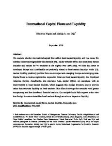
consistent with key facts about the Spanish economy, prior to the financial crisis, namely strong growth, high inflation and a deteriorating trade balance. Negative shock to Spanish housing risk premium (positive house price bubble), Fig. 2.a. A fall in the Spanish housing risk premium ztH (see (2)) raises Spanish residential investment and the Spanish house price. The housing boom crowds out private consumption (as households devote a greater share of their income to the purchase of new houses), and hence the saving rate (saving/GDP) rises. Non-residential investment rises weakly on impact, before falling persistently below the unshocked path. This is due to the fact that Spanish real interest rates fall in the short term, due to the rise in Spanish inflation, but rise over the medium term (as the price level reverts towards its pre-shock path). However, the total investment rate (total investment/GDP) rises strongly, due to the much more pronounced rise in residential investment, and the trade balance falls. Negative shock to risk premium on non-residential capital, Fig. 2.b. A fall in the risk premium on Spanish non-residential capital zti (see (5),(6)) strongly raises non-residential investment and the price of capital. Consumption and residential investment are crowded out initially, but rise in the medium run (due to the persistent rise in GDP). The initial fall of consumption (and its subsequent modest rise) imply that the saving rate rises. The total investment rate rises too; the trade balance falls. Negative shock to private borrowing rate spread in Spain, Fig. 2.c. Fig. 2.c shows the effects of a negative simultaneous shock to the Spanish private borrowing c i spreads (sprt and sprt ). This shock induces a simultaneous rise in private consumption and

in residential and non-residential investment. The saving rate falls, and the investment rate increases, and thus the trade balance deteriorates. Positive shocks to Spanish household/firm loan-to-value (LTV) ratios, Fig. 2.d. & 2.e Shocks to firm LTV ratios and to household LTV ratios have different effects. However, domestic and foreign LTV ratio shocks have identical macroeconomic consequences. This follows from the fact that the Ricardian household is indifferent between lending domestically or internationally, and has free access to the international financial market. We view these model features as realistic, given the absence of exchange rate uncertainty and the high degree of financial integration in the Euro Area. In response to an expansion in the foreign LTV ratio, the constrained household/firm borrows more abroad. When a rise in domestic LTV ratios occurs, the higher loan demand is indirectly funded abroad, as the Ricardian household accommodates the rise in domestic loan demand, by borrowing abroad (or by reducing her 15

international lending). Thus, domestic and foreign LTV ratio shocks have the same effects on aggregate demand and on GDP, i.e. only total LTV ratios matter for real activity. Fig. 2.d shows that a positive shock to the credit constrained household’s LTV ratio raises aggregate consumption and residential investment, but that it crowds out nonresidential investment; the saving rate and the total investment rate fall.13 A loosening of the borrowing constraint faced by Spanish firms boosts investment in productive capital, but it (initially) crowds out consumption and residential investment (Fig. 2.e). However, the rise in non-residential investment exceeds the fall in residential investment, and thus the total investment/GDP ratio rises; due to the fall in consumption, the saving rate rises too. Positive shocks to household and firm LTV ratios both worsen the trade balance. In summary, reductions in risk premia on Spanish residential and non-residential capital, and a rise of the firm LTV ratio all raise the Spanish saving and investment rates. By contrast, a rise in the household LTV ratio lowers the saving and investment rates. A negative shock to Spanish interest rate spreads lowers the saving rate, but raises the investment rate. [INSERT FIGURE 2 ABOUT HERE] 5.3. Business cycle moments implied by posterior parameter estimates Table 2 reports model-predicted and empirical standard deviations of key Spanish, REA and ROW macroeconomic variables, as well as their correlations with Spanish GDP. The empirical statistics are based on quarterly data for 1995Q1-2013Q2. (The statistics for all variables, except net exports/GDP, pertain to logged first differences.) Empirically, the growth rates of Spanish private and government consumption and investment are more volatile than Spanish GDP growth; these variables are all positively correlated with Spanish GDP growth. Spanish net exports (normalized by GDP) are highly volatile, and weakly countercyclical. Spanish inflation (GDP deflator) is less volatile than the GDP growth rate, while the growth rate of the Spanish house price and the rate of appreciation of the Spanish effective nominal exchange rate are more volatile than GDP growth. Spanish GDP growth is positively correlated with REA GDP growth, but uncorrelated with ROW GDP growth. The estimated model captures most of these empirical regularities rather closely. In particular, it captures the fact that Spanish domestic demand components are more volatile

13

Steady state non-residential investment is twice as large as residential investment; the fall in non-residential investment and the rise in GDP dominate the rise in residential investment, and the total investment/GDP ratio falls. 16

than Spanish GDP, and it also matches the high volatility of Spanish net exports, of the Spanish house price and of the Spanish effective exchange rate. 14 [INSERT TABLE 2 ABOUT HERE] 5.4. Variance shares accounted for by different shock types Table 3 reports the percentage shares of predicted variances (of variables considered in Table 2) that are accounted for by different types of exogenous shocks. We group together related shocks, for the sake of legibility. Specifically we consider these (groups of) shocks originating in Spain: (1) Housing risk premium; (2) (Non-residential) Capital risk premium; (3) Household LTVs; (4) Firm LTVs; (5) Interest rate spreads; (6) TFP and investment efficiency (‘Technology’); (7) Price mark-up; (8) Wage mark-up; (9) Fiscal policy; (10) All shocks originating in the REA and the ROW, as well as shocks to trade flows due to changes in the Spanish final good home bias (see Section 3.2.3) are summarized in a group labeled ‘Trade’; (11) the remaining shocks are markedly less important for the main Spanish variables, and are hence combined into a category labeled ‘Other’ shocks. Spanish financial shocks (shocks to risk premia, LTV ratios and spread) explain about 20% of the variance of Spanish net exports and of growth rates of Spanish GDP and hours worked, and 12% of the variance of Spanish inflation; about half of those variance shares are accounted for by shocks to Spanish LTV ratios and interest rate spreads. Household LTV shocks account for 40% of the variance of Spanish consumption growth. Firm LTV shocks account for a non-negligible share of the variance of non-residential investment (5%), but matter very little for the other variables. About 80% of the variances of Spanish nonresidential investment growth is driven by non-residential capital risk premium (bubble) shocks, while an equivalent share of the variance of residential investment growth and of the growth rate of house prices is accounted for by housing risk premium shocks. Only about 6% of non-residential investment variance is explained by LTV and spread shocks. Trade shocks account for about 30% of the variance of Spanish GDP growth. Although foreign factors play a non-negligible role, fluctuations in Spanish real activity are thus largely driven by local factors--domestic technology shocks (8%), price mark-up shocks (12%) and fiscal policy shocks (11%) account for non-negligible Spanish GDP variance 14

The model-predicted correlation between Spanish and REA GDP growth (0.12) is positive but smaller than the empirical correlation (0.69). This reflects the assumption that shocks originating in Spain and in the REA are independent. Standard open economy models are generally unable to generate realistic cross-country output correlations, when independent shocks are assumed (e.g., Kollmann (2013)). Empirically, aggregate supply and demand shocks are positively correlated across countries. Model versions with correlated Spanish and REA shocks generate realistic cross-country output correlations. 17

shares. As Spanish GDP is much smaller than REA and ROW output, more than 98% of the variance of REA and ROW GDP growth and inflation is driven by REA and ROW shocks. [INSERT TABLE 3 ABOUT HERE] 5.5. Decomposing Spanish historical time series To quantify the role of the different shocks as drivers of historical Spanish macro data, we plot the estimated contributions of the 11 groups of shocks described in Section 5.4 to the following Spanish time series: the nominal trade balance divided by nominal GDP; nominal GDP minus private and government nominal consumption normalized by nominal GDP (referred to as ‘saving rate’ in what follows); nominal total investment divided by nominal GDP (‘investment rate’); the year-on-year GDP growth rate; the real exchange rate. See Fig. 3.a-3.e, where lines with black lozenges show the historical data. In each Figure, the horizontal line represents the steady state value (of the variable plotted in the Figure). Vertical bars above the steady state (horizontal) line represent positive shock contributions to a variable, while bars below the horizontal line represent negative contributions. Sums of all shock contributions equal the historical data. As discussed in Section 2, the dynamics of the Spanish trade balance is dominated by a sizable expansion of the investment rate during the boom period, and a subsequent sharp correction. The historical decomposition shows that negative shocks to risk premia (bubbles) on housing and non-residential capital were major drivers of the long-lasting Spanish investment boom before the 2008-09 global financial crisis (see Fig. 3.c), and thus these shocks contributed noticeably to the gradual worsening of the Spanish trade balance (Fig. 3.a). In 2007 (i.e. just before the start of the financial crisis), the bubble shocks contributed roughly -2 percentage points to the observed Spanish net exports/GDP ratio of close to -6%. (The housing risk premium shock was the main driver of the expansion of residential investment and of the real house price in Spain, while the non-residential capital risk premium shock was the main driver of the rise in non-residential investment.) Shocks to LTV ratios too had a noticeable effect on saving, investment and the trade balance, during the boom phase. For the saving rate and the trade balance, the household LTV ratio shocks mattered more than firm LTV shocks. According to our estimates, the late 1990s saw a tightening of household LTV ratios, as is evident from the growing positive contribution of household LTV shocks to the Spanish saving rate (Fig. 3.b) and trade balance between 1997 and 1999. However, after 1999 (launch of the Euro), the estimates indicate a

18

gradual loosening in household LTV constraints that lasted until the financial crisis.15 During the global financial crisis, a sharp tightening of household LTV constraints occurred. According to the estimates, firm LTV constraints too tightened in the late 1990s and then loosened gradually. (This manifested itself in a negative contribution of the firm LTV shocks to saving and investment rates in the late 1990s that subsequently became less negative, and then turned positive in 2004.) However, that loosening only had a non-negligible positive effect on the saving and investment rates in the last two years before the financial crisis—and even then its effect on the trade balance remained very modest. During the boom phase, the convergence of Spanish rates to REA rates (i.e. negative shocks to Spanish borrowing rate spreads) had a sizable and persistent negative effect on the Spanish saving rate, and a smaller positive effect on the investment rate; thus, the spread shocks made a significant and persistent contribution to the deterioration of the Spanish trade balance, during that phase: between the late 1990s and the financial crisis, the spread shocks lowered the Spanish trade balance/GDP ratio by about 2.3 percentage points. Our estimates suggest that the expansion in Spanish loan demand triggered by the housing and non-residential capital bubbles and by falling spreads was not counteracted by a tightening of LTV ratios; given the magnitude of asset price increases, the resulting credit expansion was substantial. Especially after 2004 we even identify a sizable ‘active’ credit loosening, in the form of a marked rise in LTV ratios, that accentuated the worsening of the Spanish trade balance. According to our estimates, technology or fiscal policy shocks only had a very minor influence on Spanish saving and investment rates in the boom phase. Negative risk premium shocks and the loosening of LTV constraints also contributed noticeably to strong Spanish GDP growth before the financial crisis (see Fig. 3.d). The boom saw strong growth in the employment of unskilled labor that was also fuelled by immigration. Hence, average Spanish labor productivity and measured TFP fell during the boom years. The model interprets the strong employment growth (accompanied by low productivity growth) as induced partly by a fall in the wage mark-up. As discussed above (and documented in Fig. 3.e), the Spanish real effective exchange rate appreciated steadily until 2009, and then depreciated until 2013. The appreciation during the boom reflects strong domestic demand driven i.a. by the fall in Spanish interest rate spreads and in housing risk premia, as well as the rise in household LTV ratios. Low

15

Fig. 3.a. and 3.b. show that, after 1999, the contribution of the household LTV shocks to the trade balance and the saving rate became smaller, and turned negative in 2005. As discussed in Section 5.2., a rise in the household LTV ratio lowers the trade balance and the saving rate. 19

productivity growth during the boom also contributed to high Spanish inflation and the real exchange rate appreciation (but low wage mark-ups had an offsetting effect on inflation). The 2008-09 ‘Great Recession’ was characterized by a strong decline of the Spanish investment rate. Our estimates suggest that this was largely driven by a rise in housing and non-residential capital risk premia that triggered a fall in the value of capital. In addition, household LTV constraints tightened sharply in 2008. This combination of shocks explains also the relatively modest fall of the Spanish savings rate in 2008-2009. Due to the strong decline of investment, the trade balance improved markedly in 2008 (the global trade collapse during the recession also contributed to this). The 2008-09 drop in Spanish GDP too is mostly explained by the financial factors--in particular by a tightening of household LTV constraints, and the rise in risk premia on housing and non-residential capital. Firm credit constraints tightened later and more gradually, and contributed much less to the slump. While the non-residential investment/GDP ratio began to recover gradually after 2009, residential investment (and house prices) continued to fall after 2009 and thus exerted a drag on total investment and on GDP over the whole remaining period. In addition, Spanish interest rate spreads started to rise during the 2010-11 sovereign debt crisis. However, financial shocks only explain a small part of the persistent Spanish output slump, in the aftermath of the 2008-09 recession. Our estimates suggest that, after 2009, fiscal austerity, and a rise in price and wage mark-ups too had a strong negative effect on GDP growth.16 While the fall of the total investment rate continued to contribute to external rebalancing, in the aftermath of the 2008-09 recession, a drop in the saving rate partly offset the fall in the investment rate. (Two major facts explain the fall in the saving rate, namely the continued fall in house price, and the muted fall in Spanish wages, interpreted in the model as a rise in the wage mark-up, that stabilizes the consumption of credit-constrained households.) After 2010, Spanish net exports were also positively affected by a rise in export demand, due to the gradual recovery of the world economy, and by strong Spanish productivity growth--these factors also had a positive influence on GDP growth, and on the saving rate (as collateral constraints and habit persistence dampen the expansion of consumption, in response to a positive productivity shock). [INSERT FIGURE 3 ABOUT HERE]

16

The model predicts that GDP falls when price and wage mark-ups rise. The negative contribution of mark-up increases to GDP growth during and after the recession is clearly noticeable in Fig. 3.d. Spanish firm-level micro data also suggest a rise in price mark-ups after the financial crisis; see Montero and Urtasun (2013). 20

5.6. Sensitivity analysis: the role of shocks to risk premia and to loan-to-value ratios We also estimated a model variant without housing and non-residential capital risk premium (bubble) shocks. That model variant fits the observables less well than the baseline model. The log marginal likelihood (ML) of the baseline model is 5356.34, while the log ML of the model variant without bubble shocks is 5210.14. (The ML measures the out-of-sample predictive ability of the model.) This implies a Bayes factor (ratio of posterior odds to prior odds) of e146.20 that massively favors the baseline model. In the ‘no-bubbles’ model variant, the estimated variances of household and firm LTV ratios are close to 100%, and thus unrealistically large. The predicted standard deviations of the GDP growth rate (0.81%), residential investment growth (7.90%), the net exports/GDP ratio (4.43%) and of other key macro variables are larger than in the baseline model, and hence less close to the empirical moments (0.66%, 2.82% and 3.74%, respectively), which also indicates that the ‘no-bubbles’ variant fits the data less closely. In addition, we considered a model variant with constant household and firm LTV ratios (while allowing for residential and non-residential bubble shocks). The log ML of that model variant is 5314.24. Hence, that variant too fits the observables less well than the baseline model—though better than the ‘no-bubbles’ model variant. Compared to the baseline model, the model version without LTV shocks likewise generates predicted standard deviations of key macro variables that are larger and less close to the data (predicted standard deviations of GDP and residential investment growth, and of the net exports/GDP ratio: 0.80%, 3.39% and 5.99%). Overall, these experiments suggest that residential and non-residential capital risk premium shocks are more important than exogenous LTV ratio shocks for explaining the volatility of real activity.

6. Concluding remarks This paper has used an estimated three-country New Keynesian model with financial frictions to study the joint dynamics of foreign capital inflows and real activity during the recent boombust cycle of the Spanish economy. The estimates suggest that a falling risk premium on Spanish housing capital, a loosening of collateral constraints for Spanish households and firms, as well as the fall in the interest rate spread between Spain and the REA fuelled the persistent rise in foreign capital flows to Spain during the boom that preceded the global financial crisis. During and after the global financial crisis, falling house prices, and a tightening of collateral constraints for Spanish borrowers contributed to a sharp reduction in capital flows to Spain, and to a persistent slump in Spanish real activity. The credit crunch 21

was especially pronounced for Spanish household; firm credit constraints tightened later and more gradually, and contributed much less to the slump.

Data Appendix The model is estimated using GDP (real and deflator) growth rates and GDP (real and nominal) shares. Specifically, the following 39 variables are used as observables: ●GDP growth (3) (Spain, REA and ROW), ●GDP shares (13): trade balances (Spain, REA, ROW), consumption, government consumption, government investment, transfers, construction investment, total investment, government deficit and debt, net foreign asset, loans to firms. ●Prices (10): GDP (Spain, REA, ROW), consumption, import, export, construction, house, government purchases, total investment. ●Spain, REA, Euro-Area and ROW (US) money market rates (3 months); Spanish government bond rates; Spanish household and firm loan rates (7). ●Effective exchange rates (Spain and REA), wages, employment, number of retirees and number of labor market non-participants (6). The effective exchange rate, the ROW price index and ROW GDP are based on trade-weighted averages across Spain's main trade partners. Data sources: Eurostat, ECB, Bank of Spain.

22

References Adalet, M., B. Eichengreen (2007). Current account reversals--always a problem?, In: R. Clarida (ed.), ‘G7 Current Account Imbalances,’ University of Chicago Press. Adam, K.. P. Kuan, A. Marcet (2011). House price booms and the current account. NBER Macroeconomics Annual 2011, vol. 26, 77–122. Adjemian, S., H. Bastani, M. Juillard, F. Mihoubi, G. Perendia, M. Ratto, S. Villemot (2011). Dynare: reference manual, Version 4, Dynare Working Paper 1. Aizenman, J., Y. Jinjarak (2013). Real estate valuation, current account and credit growth patterns, before and after the 2008-09 crisis. NBER Working Paper No 19190. Bernanke, B., M. Gertler (1999). Monetary policy and asset price volatility. Federal Reserve Bank of Kansas City Economic Review 1999 4, 17-51. Calza, A., T. Monacelli, L. Stracca (2013). Housing finance and monetary policy. Journal of the European Economic Association 11, 101-122. Calvo, G. (1983). Staggered prices in a utility-maximizing framework. Journal of Monetary Economics 12, 383–398. Calvo, G. (1998). Capital flows and capital-market crises: the simple economics of sudden stops. Journal of Applied Economics 1, 35-54. Chinn, M., B. Eichengreen, H. Ito (2013). A forensic analysis of global imbalances. Working Paper, University of Wisconsin. Eggertsson, G., P. Krugman (2012). Debt, deleveraging, and the liquidity trap: a FisherMinsky-Koo approach. Quarterly Journal of Economics 127, 1469-1513. Erceg, C., L. Guerrieri, C. Gust (2006). SIGMA: a new open economy model for policy analysis. International Journal of Central Banking 2, 1–50 Fernández-Villaverde, J., L. Garicano, T. Santos (2013). Political credit cycles: the case of the Eurozone. Journal of Economic Perspectives 27, 145-166. Gomes, S., P. Jacquinot, M. Pisani (2012). The EAGLE: a model for policy analysis of macroeconomic interdependence in the Euro Area. Economic Modelling 29, 1686–1714. Gorton, G. (2010). Slapped by the invisible hand: the panic of 2007. Oxford University Press. Guerrieri, V., G. Lorenzoni (2012). Credit crises, precautionary savings and the liquidity trap. Working Paper, Northwestern University. Hale, G., M. Obstfeld (2014). The Euro and the geography of international debt flows. NBER Working Paper 20033. Hall, R. (2011). The high sensitivity of economic activity to financial frictions. Economic Journal 121, 351-378. 23

Hobza, A., S. Zeugner (2014). Current accounts and financial flows in the Euro Area. Forthcoming, Journal of International Money and Finance. Hott, C., T. Jokipii (2012). Housing bubbles. Working Paper, Swiss National Bank. Hürtgen, P., R. Rühmkorf (2014). Sovereign default risk and state-dependent twin deficits. Forthcoming, Journal of International Money and Finance in’t Veld, J., R. Raciborski, M. Ratto, W. Roeger (2011). The recent boom-bust cycle: the relative contribution of capital Flows, credit Supply and asset bubbles. European Economic Review 55, 386-406. in’t Veld, J., A. Pagano, R. Raciborski, M. Ratto, W. Roeger (2012). Imbalances and rebalancing scenarios in an estimated structural model for Spain, European Economy Economic Papers 458. Jermann, U., V. Quadrini (2012). Macroeconomic effects of financial shocks. American Economic Review 102, 238-271. Justiniano, A., G. Primiceri, A. Tambalotti (2013). Household leveraging and deleveraging. Working Paper, Federal Reserve Bank of Chicago. Justiniano, A., G. Primiceri, A. Tambalotti (2014). The effects of the saving and banking glut on the U.S. economy. Journal of International Economics 92, S52-S67. Kiyotaki, N., J. Moore (1997). Credit cycles. Journal of Political Economy 105, 211-248. Kollmann, R. (1998). U.S. trade balance dynamics: the role of fiscal policy and productivity shocks. Journal of International Money and Finance 17, 637-669. Kollmann, R. (2001). The exchange rate in a dynamic-optimizing business cycle model with nominal rigidities. Journal of International Economics 55, 243-262. Kollmann, R. (2002). Monetary policy rules in the open economy: effects on welfare and business cycles. Journal of Monetary Economics 49, 989-1015. Kollmann, R., Z. Enders, G. Müller (2011). Global banking and international business cycles. European Economic Review 55, 407-426. Kollmann, R., W. Roeger, J. in’t Veld (2012). Fiscal policy in a financial crisis: standard policy vs. bank rescue measures. American Economic Review 102, 77-81. Kollmann, R. (2013). Global banks, financial shocks and international business cycles: evidence from an estimated model. Journal of Money, Credit and Banking 45, 159-195. Kollmann, R., M. Ratto, W. Roeger and J. in’t Veld (2013). Fiscal Policy, Banks and the Financial Crisis. Journal of Economic Dynamics and Control 37, 387-403. Kollmann, R., M. Ratto, W. Roeger, J. in’t Veld, L. Vogel (2014). What drives the German current account? And how does it affect the other EU member states? CEPR DP 9933. 24

Montero, J., A. Urtasun (2013). Recent developments in non-financial corporations’ markups. Bank of Spain Economic Bulletin (December), 3-10. Obstfeld, M., K. Rogoff (2010). Global imbalances and the financial crisis: products of common causes. In: Asia and the Global Financial Crisis. San Francisco Fed, pp.131-172. Ratto M., W. Roeger, J. in ’t Veld (2009). QUEST III: an estimated open-economy DSGE model of the Euro Area with fiscal and monetary policy. Economic Modelling 26, 222-233. Reis, R. (2013). The Portuguese slump-crash and the Euro Crisis. Brookings Papers on Economic Activity, 143-193. Smets, F., R. Wouters (2007). Shocks and frictions in US business cycles: a Bayesian DSGE approach. American Economic Review, 97, 586-606.

25

Table 1. Prior and posterior distributions of key model parameters Prior distributions Distribution Mean (1)

(2)

s.d.

(5)

(6)

0.73 1.31 0.56

0.05 0.39 0.11

Steady state consumption share of Ricardian households C r /C Beta 0.50 0.10

0.52

0.05

Autocorrelations of forcing variables  ( c,d ) Beta 0.85

0.07

0.88

0.06

Household preferences Beta  Gamma  Gamma 

 ( c, f )  (  i ,d )  (  i, f )  ( spr c )  ( spri )

(3)

(4)

0.70 1.00 0.50

0.10 0.40 0.10

Posterior distributions Mean s.d.

Beta

0.85

0.07

0.90

0.05

Beta

0.85

0.07

0.86

0.08

Beta

0.85

0.07

0.92

0.04

Beta

0.85

0.07

0.84

0.05

Beta

0.85

0.07

0.93

0.01

Standard deviations (%) of innovations to forcing variables sd ( c,d ) Gamma 4.0 1.6

5.58

2.38

sd ( c, f )

Gamma

4.0

1.6

5.85

1.84

sd (  ) sd (  i , f ) sd ( spr c )

Gamma

4.0

1.6

4.16

1.65

Gamma

4.0

1.6

5.87

1.94

Gamma

1.0

0.3

0.83

0.19

sd ( spr i )

Gamma

1.0

0.3

0.92

0.92

i ,d

Notes: Cols. (1) lists model parameters;  (x), sd (x) are the autocorrelation of variable ‘x’ and the standard deviation of the innovation to x, respectively.  c ,d and  c , f are exogenous LTV ratios facing Spanish credit constrained households when borrowing from domestic and foreign lenders, respectively.  i ,d and  i , f : corresponding domestic and foreign LTV ratios for Spanish intermediate good producing firms. spr c and spr i : interest rate spreads for loans to the Spanish credit-constrained household and intermediate goods-producing firms. Col. (2) shows the distribution functions of the priors. Cols. (3),(4): means and the standard deviations (s.d.) of the prior distributions of parameters. Cols. (5),(6): means and standard deviations of the posterior parameter distributions (based on Random Walk Metropolis algorithm, 400000 draws).

26

Table 2. Model-predicted and empirical business cycle statistics (1995Q1-2013Q2)

Model Standard deviation, % (1)

Data

Correl. with Spanish GDP

Standard deviation, %

Correl. with Spanish GDP

(2)

(3)

(4)

(5)

Spanish variables GDP Consumption (private) Government consumption Non-residential investment Residential investment Hours worked Net exports/GDP

0.74 1.07 1.46 3.00 4.14 0.74 3.94

1.00 0.51 0.41 0.49 0.46 0.75 -0.03

0.66 0.91 1.09 2.82 3.15 0.93 3.74

1.00 0.80 0.34 0.73 0.72 0.92 -0.15

Nominal exchange rate GDP deflator House price

4.44 0.77 2.54

-0.20 0.10 0.15

4.20 0.48 2.59

-0.04 0.60 0.58

REA variables GDP GDP deflator

0.85 0.39

0.12 0.13

0.64 0.30

0.69 -0.03

ROW variables GDP GDP deflator

1.00 2.09

0.19 0.17

0.79 1.89

0.07 0.22

Note: For the variables listed in Column (1), the Table reports model-predicted standard deviations and correlations with Spanish GDP (Columns (1)-(2)) and the corresponding empirical statistics based on quarterly data for the period 1995Q1-2013Q2 (Columns (3)-(4)). The statistics for all variables except net exports/GDP pertain to logged first differences of these variables. ‘Inflation’ is a quarter-to-quarter rate. The ‘Nominal exchange rate’ is the effective exchange rate between Spain and the ROW (a rise represents a Spanish appreciation). REA: Rest of Euro Area (EA less Spain); ROW: Rest of world.

27

Table 3. Shares (in %) of model-predicted variances accounted for by different shock types Financial shocks Housing Capital Houserisk risk hold Firm premium premium LTV LTV (1)

(2)

Interest rate Tech- Price spreads nology mark-up

(14)

Trade

Other

(10)

(11)

(12)

(13)

12.40 2.89 5.74 3.37 0.41 16.84 3.64

4.80 0.71 8.82 0.83 0.21 13.25 4.56

11.10 0.90 61.79 0.19 0.07 4.80 7.38

29.86 20.45 8.22 7.95 1.17 19.45 54.68

14.88 22.53 4.90 1.08 9.96 18.13 4.14

18.95 49.86 7.69 85.70 88.03 21.22 24.60

9.03 43.06 2.65 6.29 6.00 10.54 14.95

16.64 0.68 0.04

25.11 0.41 0.00

17.62 0.48 0.01

2.55 0.13 0.02

19.78 2.32 98.62

6.43 21.41 1.23

11.84 74.55 0.07

7.12 0.26 0.03

0.00 0.84

0.04 0.39

0.02 0.11

0.01 0.19

0.01 0.41

98.29 95.14

1.57 2.13

0.03 1.60

0.01 0.99

0.00 0.00

0.03 0.13

0.00 0.00

0.00 0.00

0.00 0.00

99.97 99.86

0.00 0.00

0.00 0.00

0.00 0.00

(4)

(5)

(6)

(7)

(8)

5.80 0.74 1.21 79.18 0.07 5.18 2.89

7.98 40.26 1.84 0.43 5.61 9.43 4.68

0.38 0.47 0.24 5.04 0.04 0.33 0.62

0.66 2.32 0.56 0.81 0.34 0.77 9.65

7.98 2.63 2.79 0.84 0.12 6.28 0.98

2.48 74.24 0.03

2.24 0.04 0.01

6.28 0.20 0.00

0.18 0.01 0.00

0.65 0.05 0.03

REA variables GDP GDP deflator

0.02 0.47

0.00 0.14

0.01 0.11

0.00 0.03

ROW variables GDP GDP deflator

0.00 0.00

0.00 0.00

0.00 0.00

0.00 0.00

GDP deflator House price Nominal Exchange rate

Fiscal policy

LTV & spread shocks

(9)

(3)

Spanish variables GDP 4.11 Consumption (private) 6.05 Government consumption 3.82 Non-residential investment 0.22 Residential investment 81.95 Hours worked 5.49 Net exports/GDP 6.74

Wage mark-up

All financial shocks

Note: this Table reports % shares of the model-predicted variances of variables listed in Column (1) that are accounted for by the types of shocks listed above Columns (2)-(14). The sum of the shares listed in Columns (2)-(13) is 100%. Column (13) reports the variance share explained by financial shocks (Columns (2)(6)), while Column (14) shows the variance share explained by LTV shocks and by shocks to Spanish interest rate spreads (sum of Columns (4)-(6)). See Section 5.4 for discussion of shock types. The variances of all variables except net exports/GDP pertain to logged first differences of these variables. ‘Inflation’ is a quarter-to-quarter rate. The ‘Nominal exchange rate’ is the effective exchange rate between Spain and the ROW (a rise represents a Spanish appreciation). REA: Rest of Euro Area (EA less Spain); ROW: Rest of world.

28

Figure 1 Spain: 1995Q1-2013Q2 Fig. 1.a. Year-on-year GDP growth (%): Spain and REA

Fig. 1.b Real demand shares % (ratios to real GDP, base yr. 2000)

I [IH]: non-residential [housing] investment; C: consumption Fig. 1.c Trade balance (TB), current account (CA) and gov’t deficit (GOC), % GDP

Fig. 1.d Savings, investment, net exports, % GDP

Fig. 1.e Net foreign claims against Spanish sectors, % GDP

Fig. 1.f Nominal interest rates,% p.a.

BoS: Bank of Spain, GOV: general government; HH: households; Corp: private corporations

Borrowing rates: Spanish households (HH), non-fin. firms (NFC), government (GOV). Bank of Spain (BoS) & ECB policy rates

Fig. 1.g YoY Growth of GDP deflator and house price, %

29

Figure 2. Impulse responses to financial shocks Figure 2.a. Negative shock to Spanish housing risk premium GDP

Consumption

0.35

Non-residential Investment 0.05

0.02

0.3

6 0

0

-0.02

-0.05

-0.04

-0.1

-0.06

-0.15

-0.08

-0.2

0.25

5

0.2 0.15

4 3

0.1

2

0.05 0

Residential Investment 7

1

10

20

30

40

10

Employment

20

30

40

Trade balance (% GDP)

0.35

0

0.3

-0.01

0.25

-0.02

0.2

-0.03

0.15

-0.04

10

20

30

40

Real effective exchange rate 0.3 0.25

0

10

20

30

40

Real interest rate (bp) 5 0

0.2

-5

0.15 -10 0.1 -15 0.05 0.1

-0.05

0.05

-0.06

0

10

20

30

40

-20

0

-25

-0.05

-0.07

10

20

30

40

-0.1

10

20

30

40

-30

10

20

30

40

Figure 2.b Negative shock to risk premium on Spanish non-resident capital GDP

Consumption

0.4

Non-residential Investment 5

0.15 0.1

0.3

Residential Investment 0.2 0.15

4

0.05

0.1

0

3

-0.05

2

0.05

0.2

0.1

-0.05 1

-0.15 0

0

-0.1

10

20

30

40

-0.2

Employment

10

20

30

40

Trade balance (% GDP)

0.35

0

0.3 -0.05

0.25 0.2

0

-0.1 10

20

30

40

-0.15

Real effective exchange rate 0.2

30

0.1

20

0

10

-0.1

0

-0.2

-10

10

20

30

40

Real interest rate (bp)

-0.1 0.15 0.1

-0.15

0.05 0

10

20

30

40

-0.2

10

20

30

40

-0.3

10

20

30

40

-20

10

20

30

40

Figure 2.c. Negative shock to Spanish private interest rate spread GDP

Consumption

0.07

Non-residential Investment 0.35

0.2

0.06

0.3 0.15

0.05

Residential Investment 0.25 0.2

0.25

0.04

0.2

0.15

0.15

0.1

0.1 0.03 0.02

0.1

0.05

0.01 0

0.05

0.05 10

20

30

40

0

Employment

10

20

30

40

Trade balance (% GDP)

0.07

0

0.06

-0.01

0.05

-0.02

0.04

-0.03

0.03

0

10

20

30

40

Real effective exchange rate 0.12

0

10

20

30

40

Real interest rate (bp) 0

0.1

-2

0.08

-4

0.06

-6

0.04

-8 -10

-0.04

0.02

-0.05

0.01

-0.06

0.02

0

-0.07

0

10

20

30

40

10

20

30

40

30

10

20

30

40

-12

10

20

30

40

Figure 2.d. Positive shock to Spanish household foreign loan-to-value ratio GDP

Consumption

Non-residential Investment 0.1

1

0.25

0.8

0.2

Residential Investment 1.2 1

0

0.6

0.8

0.15

0.4

-0.1

0.6

0.1

0.2

-0.2

0.4

0 0.05 0

0.2 -0.3

-0.2 10

20

30

40

-0.4

Employment

10

20

30

40

Trade balance (% GDP)

0.35

0.15

0

-0.4

10

20

30

40

-0.2

Real effective exchange rate 0.3

20 10

0.3

0.1

0.2

0.25

0.05

0.1

0.2

0

0

10

20

30

40

Real interest rate (bp)

0 -10

0.15

-0.05

-0.1

0.1

-0.1

-0.2

0.05

-0.15

-0.3

0

-0.2

-0.4

10

20

30

40

10

20

30

40

-20 -30

10

20

30

40

-40

10

20

30

40

Figure 2.e. Positive shock to Spanish firm foreign loan-to-value ratio GDP

Consumption

0.12

Non-residential Investment 1.4

0.04

Residential Investment 0.05

1.2

0.1 0.02

1

0.08

0.8 0.06

0

0 0.6

0.04

0.4

-0.02 0.02 0

0.2 10

20

30

40

-0.04

Employment

10

20

30

40

Trade balance (% GDP)

0.06

0

0.05

-0.005

0.04

-0.01

0.03

-0.015

0

10

20

30

40

Real effective exchange rate 0.02

-0.05

10

20

30

40

Real interest rate (bp) 4 3

0

2 -0.02 1 -0.04

0.02

-0.02

0.01

-0.025

0

10

20

30

40

-0.03

0 -0.06

10

20

30

40

-0.08

-1

10

20

30

40

-2

10

20

30

40

Note: A Spanish real appreciation is represented by a rise in the real exchange rate. The ‘real interest rate’ is the real household loan rate.

31

1.4 0.8 1.3 0.7

Figure 3. Historical decompositions Figure 3.a. Spain: trade balance/GDP quarter to quarter ES_TBYN

1995

1996

1997

1998

1999

2000

2001

2002

2003

2004

2005

1.2 Housing risk premium

0.06

Capital risk premium 1.1

0.04

Household LTVs Firms LTVs

0.02

Interest rate spreads

1

0

Technology

Price markup quarter to quarter ES_REE Wage markup

-0.02

0.9 1.5 -0.04

Fiscal policy Trade

-0.06

0.8 1.4

Others

-0.08 1995

1996

1997

1998

1999

2000

2001

2002

2003

2004

2005

2006

2007

Technology Stock market risk premium

2008

2009

0.7 1.3 1995

1996

2010

1997

2011

2012

1998

2013

1999

2000

2001

2002

2003

2004

2005

2

2005

2

Firms financing conditions Figure 3.b. Spain: (GDP-private consumption-government consumption)/GDP quarter to quarter ES_SY Housing risk premium Household financing conditions

0.32

0.3

Capital risk premium Household LTVs

Wage restraint Fiscal shocks

0.28

Housing risk premium

1.2

Trade shocks Price markup Risk premia shocks

1.1

Firms LTVs

Others

Interest rate spreads

0.26

Technology

1

0.24

Price markup 0.22

Wage markup 0.9

0.2

Fiscal policy Trade

0.18

Others

0.8 0.16

1995

1996

1997

1998

1999

2000

2001

2002

2003

2004

2005

2006

2007

2008

2009

2010

2011

2012

2013

Technology

0.7

Stock market risk premium Firms financing conditions

1995

1996

1997

1998

1999

2000

2001

2002

2003

2004

Figure 3.c. Spain: total investment/GDP

Housing risk premium Household financing conditions quarter to quarter ES_ITOTSN

0.32

Trade shocks Price markup Risk premia shocks

0.3

Housing risk premium Capital risk premium

Wage restraint Fiscal shocks

0.28

Household LTVs

Others

Firms LTVs 0.26

Interest rate spreads 0.24

Technology

0.22

Price markup Wage markup

0.2

Fiscal policy 0.18

Trade Others

0.16

0.14

1995

1996

1997

1998

1999

2000

2001

2002

2003

2004

2005

2006

2007

Technology Stock market risk premium Firms financing conditions Housing risk premium Household financing conditions Trade shocks Price markup Risk premia shocks Wage restraint Fiscal shocks Others

32

2008

2009

2010

2011

2012

2013

0.8 1.4

0.7 1.3

1995

1996

1997

1998

1999

2000

2001

2002

2003

2004

2005

2

2005

2

3.d. Spain: year-on-year GDP growth year on year ES_GY 0.08

Housing risk premium

1.2

Capital risk premium

0.06

Household LTVs 1.1

0.04

Firms LTVs Interest rate spreads

0.02

Technology

1 0

Price markup Wage markup

-0.02

0.9

Fiscal policy Trade

-0.04

-0.08

Others

0.8

-0.06

1996

1997

1998

1999

2000

2001

2002

2003

2004

2005

2006

2007

2008

0.7

1995

2009

1996

2010

1997

2011

2012

1998

2013

1999

2014

2000

2001

2002

2003

2004

Figure 3.e. Spain: log real exchange rate (deviation from steady state) Technology quarter to quarter ES_REER

0.5

Stock market risk premium Firms financing conditions Housing risk premium Household financing conditions Trade shocks Price markup Risk premia shocks Wage restraint Fiscal shocks Others

0.4

0.3

0.2

Housing risk premium Capital risk premium Household LTVs Firms LTVs Interest rate spreads Technology

0.1

Price markup Wage markup

0

Fiscal policy -0.1

Trade Others

-0.2

-0.3

1995

1996

1997

1998

1999

2000

2001

2002

2003

2004

2005

2006

2007

2008

2009

2010

2011

2012

2013

Technology Stock market risk premium Firms financing conditions Housing risk premium Household financing conditions

Note: The lines with black lozenges show the historical data. Thin horizontal line represents steady state values. Vertical bars show contributions of different types of shocks to the historical data. Vertical bars above the horizontal (steady state) line represent positive shock contributions to the historical data, while bars below the horizontal line represent negative contributions. The (groups of) shocks are describes in Section 5.4. In Fig. 3.e, a Spanish real exchange rate appreciation is represented by a rise in the real exchange rate. Trade shocks Price markup

Risk premia shocks Wage restraint Fiscal shocks Others

33