INTENSITY-RESOLVED ABOVE THRESHOLD IONIZATION YIELDS OF ATOMS WITH ULTRASHORT LASER PULSES
A Thesis by NATHAN ANDREW HART
Submitted to the Office of Graduate Studies of Texas A&M University in partial fulfillment of the requirements for the degree of MASTER OF SCIENCE
August 2011
Major Subject: Physics
Intensity-resolved Above Threshold Ionization Yields of Atoms with Ultrashort Laser Pulses Copyright 2011 Nathan Andrew Hart
INTENSITY-RESOLVED ABOVE THRESHOLD IONIZATION YIELDS OF ATOMS WITH ULTRASHORT LASER PULSES
A Thesis by NATHAN ANDREW HART
Submitted to the Office of Graduate Studies of Texas A&M University in partial fulfillment of the requirements for the degree of MASTER OF SCIENCE
Approved by: Co-Chairs of Committee, Gerhard Paulus Alexandre Kolomenski Committee Members, Hans Schuessler Winfried Teizer Stephen Fulling Head of Department, Edward Fry
August 2011
Major Subject: Physics
iii
ABSTRACT
Intensity-resolved Above Threshold Ionization Yields of Atoms with Ultrashort Laser Pulses. (August 2011) Nathan Andrew Hart, B.S., Texas A&M University Co-Chairs of Advisory Committee: Dr. Gerhard Paulus Dr. Alexandre Kolomenski
The above threshold ionization (ATI) spectra provide a diversity of information about a laser-atom ionization process such as laser intensity, pulse duration, carrier envelope phase, and atomic energy level spacing. However, the spatial distribution of intensities inherent in all laser beams reduces the resolution of this information. This research focuses on recovering the intensity-resolved ATI spectra from experimental data using a deconvolution algorithm. Electron ionization yields of xenon were measured for a set of laser pulse intensities using a time of flight (TOF) setup. Horizontally polarized, unchirped, pulses were used in the ionization process. All laser parameters other than the radiation intensity were held constant over the set of intensity measurements. A deconvolution algorithm was developed based on the experimental parameters. Then the deconvolution algorithm was applied to the experimental data to obtain the intensity-resolved total yield probability and ATI spectra. Finally, an error analysis was performed to determine the stability and accuracy of the algorithm as well as the quality of the data.
iv
It was found that the algorithm produced greater contrast for peaks in the ATI spectra where atom specific resonant behavior is observed. Additionally, the total yield probability showed that double ionization may be observed in the ionization yield. The error analysis revealed that the algorithm was stable under the experimental conditions for a range of intensities.
v
DEDICATION
To my Lord and Savior Jesus Christ.
vi
ACKNOWLEDGEMENTS
I would like to thank my advisor, Dr. Gerhard Paulus, and Dr. Hans Schuessler for their advice and for making this research possible. Additionally, I would like to thank the co-chair of my committee, Dr. Alexandre Kolomenski, for his guidance concerning my research and the completion of this thesis. To the committee members, Dr. Stephen Fulling and Dr. Winfreid Tiezer, I am grateful for all their time and help. I would like to thank Dr. James Strohaber for detailed discussions and assistance related to this experiment. I acknowledge the Department of Physics at Texas A&M and the US Air Force for their financial support over the past few years. It has been a privilege to work in the Attosecond and Fewcycle Laser Laboratory with Fransisco Pham, Feng Zhu, Ricardo Nava, Necati Kaya, Gamze Kaya and Cade Perkins. I would like to thank my ReJOYce IN JESUS family for their prayers. And finally, a special thanks goes to my mother, father and sister for their encouragement and support.
vii
TABLE OF CONTENTS
Page ABSTRACT ..................................................................................................................... iii DEDICATION ................................................................................................................... v ACKNOWLEDGEMENTS .............................................................................................. vi TABLE OF CONTENTS .................................................................................................vii LIST OF FIGURES ...........................................................................................................ix 1. INTRODUCTION AND LITERATURE REVIEW ..................................................... 1 2. IONIZATION OF ATOMS ........................................................................................... 3 A. Ponderomotive Energy.......................................................................................... 3 B. Multiphoton Ionization.......................................................................................... 7 C. Tunneling Ionization ............................................................................................. 9 D. Over the Barrier Ionization ................................................................................. 10 E. Above Threshold Ionization ................................................................................ 12 3. SCHEME FOR REALIZATION OF INTENSITY-RESOLVED IONIZATION RATES ......................................................................................................................... 15 A. Basic Principle .................................................................................................... 15 B. Experimental Setup ............................................................................................. 15 C. Experimental Equipment ..................................................................................... 17 4. CONVERTING FROM TOF TO ENERGY SPECTRA ............................................ 20 A. The Format of Recorded Data............................................................................. 20 B. Discrete Conversion to Energy Spectra .............................................................. 22 C. Continuous Conversion to Energy Spectra ......................................................... 22 5. GAUSSIAN BEAM GEOMETRY ............................................................................. 24 6. REMOVING INTENSITY INTEGRATION .............................................................. 26 A. Intensity Difference Scanning............................................................................. 26 B. Analytical Volume Deconvolution in M Dimensions ......................................... 30 C. Implementation of the Volume Deconvolution................................................... 32 D. Error Propagation Through the Algorithm ......................................................... 33 E. Runge’s Phenomenon .......................................................................................... 35 7. ANALYSIS OF EXPERIMENTAL DATA ................................................................ 37
viii
Page 8. SUMMARY AND CONCLUSION ............................................................................ 42 REFERENCES ................................................................................................................. 43 VITA ................................................................................................................................ 45
ix
LIST OF FIGURES
Page Fig. 1. Electrons being pushed away from the center of the focus. ................................... 4 Fig. 2. Ionization in a low intensity field. .......................................................................... 6 Fig. 3. Photon absorption and spontaneous reemission.. ................................................... 7 Fig. 4. Photoionization due to the photoelectric effect (A) and multi-photon absorption (B) .......................................................................................................... 8 Fig. 5. Tunneling Ionization ............................................................................................... 9 Fig. 6. A graphical depiction of over the barrier ionization. ............................................ 11 Fig. 7. A graphical depiction of the ATI process. Here the electron absorbs an integer number of photons whose total energy exceeds by more than one photon. .... 13 Fig. 8. Channel closing for the
and
peaks of a simulated ATI spectrum. .............. 14
Fig. 9. The experimental setup. ........................................................................................ 16 Fig. 10. A photograph taken of the ATI apparatus and related components. ................... 17 Fig. 11. The essential components of the ATI apparatus. ................................................ 18 Fig. 12. A visual representation of the time bins
and their electron counts
.. ....... 21
Fig. 13. A depiction of the three-dimensional iso-intensity shells. .................................. 25 Fig. 14. An example schematic in one dimension showing how volume elements are related to peak intensities.. .................................................................................. 27 Fig. 15. A scheme showing the relationship between the volume elements ( , , ) and their respective probabilities ( , , ) ............................. 28 Fig. 16. Graphical depiction of the IDS algorithm using two intensities. ........................ 29 Fig. 17.
and
portrayed as
matrix transformations between
and . ........ 30
Fig. 18. Interpolating polynomials of degree 5 (blue) and 9 (green) and their
x
Page generation function (red) .................................................................................... 35 Fig. 19. The photoelectron yield rate for xenon ............................................................... 37 Fig. 20. The Runge divergence calculated for the model xenon probability function using (6.26) ................................................................................................. 38 Fig. 21. The intensity-resolved probability of the data .................................................... 39 Fig. 22. Intensity-resolved ATI energy spectra at
. ........................... 40
Fig. 23. Intensity-resolved ATI energy spectra at
. ........................... 41
1
1. INTRODUCTION AND LITERATURE REVIEW
When performing experiments to study the atomic and/or molecular interaction with a laser field the detection information often comes from ionized electron or fluorescence photon signals. The signal probability is a function of the radiation intensity and wavelength where the atom or molecule is located. The focal volume of a laser contains a continuum of intensities that vary both radially and longitudinally with respect to the axis of propagation and range from zero to some peak intensity. Each intensity contributes a unique ion yield rate depending on the probability of ionization and the volume of that radiation intensity. It has been demonstrated that the position of an ion within the focus can be measured to high precision (
) (Strohaber, 2008). However, measuring devices are rarely able to
determine the location within the focus that an electron originated from. For instance, to distinguish two coaxial electrons in an electric field-free region with energy and a separation distance of with require
of kinetic
would require data acquisition electronics
resolution. For photons of the same energy and spatial separation it would temporal resolution. Typical fast data acquisition electronics have temporal
resolutions of a few hundred picoseconds. The insufficient temporal resolution results in integration of the signal over the entire focal volume of the laser.
____________ This thesis follows the style of Advances in Atomic, Molecular and Optical Physics.
2
Several methods have been employed to work around this difficulty. Hansch and Van Woerkom (1996) used a two dimensional z-axis measurement to obtain a photoelectron spectra with less intensity integration than a typical three-dimensional focal volume experiment. They noted that if a thin cross-section of a laser focus
is
taken, the ratios of volumes occupied by different intensities changes as a function of the longitudinal variable z. By choosing a
position where the desired intensity spatially
dominates, one can obtain a more selective intensity measurement. Walker et al. (1998) added an algorithm to the above z selection method to remove all radial volume integration while maintaining the small integration from the thickness of the slice
. To
do this they analytically deconvolved the volume integration in two dimensions (radial and azimuthal) to obtain the probability of ionization as a function of intensity. Bryan et. al. (2006a) improved upon this algorithm, now termed Intensity Selective Scanning (ISS), by accounting for laser diffraction effects in the focal volume. Bryan et. al. (2006b) used this improved ISS algorithm to investigate intensity resolved ionization rates of higher charged states. While they were able to find the total ionization rate for a specific intensity, they did not obtain an intensity-resolved electron spectra. The aim of this thesis is to demonstrate a deconvolution algorithm that can be used to obtain intensity-resolved photoelectron spectra. This would allow us to observe the appearance of Rabi oscillations and AC Stark shifts within the atomic energy levels.
3
2. IONIZATION OF ATOMS
A. Ponderomotive Energy A free (continuum) electron in an oscillating electric field,
̂,
absorbs kinetic energy and oscillates slightly out of phase with the field. The free electron however retains the frequency of the oscillating field since this field is the only applied force. This can be seen by defining the Lagrangian for linearly polarized continuous wave radiation: ̇
(2.1)
Plugging equation (2.1) into Lagrange’s equation of motion and integrating successively with respect to time gives the velocity and position of the “classical” electron: (2.2) ̇ where
is the drift velocity and
ionized. Using the definitions
(2.3) is the initial position of the electron when it was and
and neglecting the drift
velocity, the time averaged kinetic energy or ponderomotive energy in electron volts (
) of such an electron is: 〈 ̇ 〉
(2.4)
(2.5)
4
[
] [
]
(2.6)
This quantity is important because an electron in a finite laser beam of sufficiently long pulse duration will on average gain this energy, ̃ , in the form of translational kinetic energy. Since for a Gaussian beam the local electric field amplitude as a function of the radius in cylindrical coordinates is: (2.7) replacing
with
gives the local ponderomotive energy: ̃
(2.8)
where the azimuthal dependence has been neglected. This ponderomotive energy acts as an electric potential and provides a radial force
to the electron due to the spatial
variation in the field (see Fig. 1). ̃
Fig. 1. Electrons being pushed away from the center of the focus.
(2.9)
5
If the electron is initially at a radius
prior to being accelerated, then the work done on
the electron as it is pushed out of the field is: ∫
(2.10)
̃
(2.11)
This means that the electron will gain a translational kinetic energy equal to the ponderomotive energy where it initially experienced the field. In calculating upper bound of the integral implies that
, the
the radiation is continuous wave (CW).
However, for sufficiently short pulses the electron may not have enough time to be displaced out of the field and, as a result, not gain the full ̃
. A rough estimate of
the necessary laser parameters for equation (2.11) to hold can be obtained by equating the kinetic energy of the free electron to pulse duration
and finding the distance it travels for
. For example, a pulse of wavelength
and peak intensity
, duration
would move an electron less than
away from
the center of the beam. This is negligible compared to a typical beam waist of , and as a result the upper bound of the integral (2.10) is approximately
.
When an electric field is applied to an atom, the energy levels change by a value known as the Stark shift. Through a lengthy quantum mechanical calculation (Delone & Krainov, 1994) it is found that the dynamic or AC Stark shift of an atomic energy level due to an oscillator field is approximated by: (2.12) (2.13)
6
It is remarkable that the AC Stark shift under the above restriction is equal to the ponderomotive energy
provided by the field. One consequence of this is that the
highest “continuum” state
, is increased in the following manner:
.
To be ionized the electron must now gain an energy: (2.14) where
is the ionization energy of the unperturbed atom (see Fig. 2).
Fig. 2. Ionization in a low intensity field.
Once ionized the electron is pushed along the radiation energy gradient towards lower ponderomotive energies. For sufficiently long laser pulse durations ( intensities (
) at
) and large
the electron will regain the kinetic energy
lost through the AC Stark shift as it travels away from the atom. However, for short laser pulses (
) even intensities as high as
sufficient to recover the lost energy.
will not be
7
B. Multiphoton Ionization There are three general ways in which photoionization can be described. For the lowest intensities, a process analogous to the photoelectric effect occurs. In the photoelectric effect, an atom is ionized when a bound electron absorbs a photon whose energy
exceeds the atomic potential energy
. The photoelectric effect follows the
rule of being independent of the radiation intensity because the decay rate of the excited atom is much faster than the absorption rate of new photons. Thus, for a wide range of intensities (in Xenon:
), photons with energy
are reemitted
by the atom (see Fig. 3).
Fig. 3. Photon absorption and spontaneous reemission. The photon in red and the unexcited atom (A). The excited atom (B). Spontaneous emission of a photon (C).
However, increasing the radiation intensity the appearance intensity
above a certain threshold, called
, allows the photon absorption rate to exceed the decay rate.
It is then possible to ionize the atom through an absorption of several photons as the sum of the photon energies exceeds the ionization potential.
8
∑
(2.15)
Fig. 4. Photoionization due to the photoelectric effect (A) and multi-photon absorption (B).
This process is referred to as multi-photon ionization (MPI), and can be viewed as a generalization of the photoelectric effect (see Fig. 4). For a broadband laser the electron can absorb several photons each with a unique energy present in the spectrum. But for simplicity, equation (2.16) depicts the interaction of monochromatic radiation with the atom “ ”: (2.16) where
is the number of photons absorbed,
ejected electron,
is the prepared target, and
is the energy of each photon,
is the
is the final state of the target. The
energy of the electron is then: (2.17) where
is the potential energy of the electron for atom . The radiation field is viewed
as perturbation to the atomic potential well and perturbation theory can be used to find the ionization probability
.
is proportional to the radiation intensity
power equal to the order of the multi-photon ionization:
to the
9
(2.18) where
satisfies
.
C. Tunneling Ionization As an atom interacts with an oscillating electric field, the Coulomb potential of the initially unperturbed atom begins to sway back and forth in phase with the field. This is related to the variations of the effective potential of the atom: (2.19)
[ where
is the charge state of the atom,
the radiation field amplitude,
]
(2.20)
is the distance away from the nucleus,
is the frequency of the oscillation and
is
is the time
variable. For sufficiently large electric fields, this effective potential of the atom will “dip” down, creating a well that the bound electron can tunnel out of (see Fig. 5). This is referred to as tunneling ionization (TI).
Fig. 5. Tunneling Ionization. The electron tunnels (dashed line) out of the atom and into the continuum.
10
The average tunneling time
is determined by the potential barrier height and
thickness. The Keldysh tunneling parameter
is a metric for determining when the
intensity is high enough to describe the ionization mainly through a tunneling process. The parameter
has two equivalent representations (Keldysh, 1965): (2.21)
( where and
(2.22)
)
is the frequency of the oscillating electric field,
is the ionization potential
is the ponderomotive potential. The first representation gives an intuitive picture
of the tunneling process. If the period of the laser,
, is comparable to the tunneling
time, , then tunneling becomes probable. Hence
is a necessary but not sufficient
condition to imply electron tunneling out of the atom. The second representation is more useful for experimental research because it can be easily calculated. in published atomic and molecular reference materials and
is usually found
can be calculated from
equation (2.6). The utility of the Keldysh parameter itself comes from its ability to distinguish between MPI (
) and TI (
). However, when
approaches unity a
mixture of the two processes maybe seen in experiment because both MPI and TI become probable to occur. D. Over the Barrier Ionization If the laser intensity is large enough, the Coulomb potential may no longer be higher than the unperturbed ground state. In this case, there is no longer a bound state for
11
the outer most electron. This electron is then said to be freed through Over The Barrier Ionization (OTBI).
Fig. 6. A graphical depiction of over the barrier ionization.
To gain a qualitative understanding of the process we ignore any longitudinal electric field components of the uncollimated beam and reduce equation (2.19) to one dimension. This paraxial approximation is only valid where the beam makes a negligible angle with the axis of propagation. The minimum electric field required to induce OTBI can then be found by first noting that the condition for OTBI is the following:
| |
(2.23)
This means that the ground state energy of the unperturbed atom is greater than the peak potential energy of the atom in the radiation field (see Fig. 6). We can find equation
from the
. This gives: √
(2.24)
12
for the distance away from the nucleus where the potential starts to dip back down. Plugging equation (2.24) into equation (2.23) gives: (2.25)
(2.26) Note that while MPI and TI are functions of two laser parameters a function of
and , OTBI is only
This is because of the relatively small mass, and thus inertia, of the
electron. An unbound electron with one unit of photon energy laser cycle, travel a distance more than
times the Bohr radius
will, in half a . For comparison the
neutral xenon atom is approximately twice the Bohr radius. This means that for a wide range of photon energies the wavelength dependence is negligible. E. Above Threshold Ionization During irradiation, electrons in the target atom or molecule may absorb more photons than are needed to exceed the ionization threshold
. The absorption of
additional photon energy above the minimum ionization threshold is referred to as Above Threshold Ionization (ATI) (see Fig. 7). This is expressed mathematically by: (2.27) where
is the kinetic energy of the electron in the continuum due to photon absorption.
ATI may, and typically does occur in all three of the above mentioned ionization mechanisms (MPI, TI and OTBI).
13
Fig. 7. A graphical depiction of the ATI process. Here the electron absorbs an integer number of photons whose total energy exceeds by more than one photon. The figure shows the graph of a numerical simulation from Paulus, Nicklich, Zacher, Lambropoulos, & Walther (1996) superimposed on to a drawing of an atomic potential well.
If the intensity of the radiation is large, such that the energy of the electron is: (2.28) (2.29) the electron will not escape the atom and thus will not appear in the ATI spectrum. As intensity increases, the AC Stark shift (2.13) may exceed the energy of the lower energy peaks successively (see Fig. 8). In such a case, channel closing is said to have occurred and the respective peaks appear suppressed.
14
Fig. 8. Channel closing for the
and
peaks of a simulated ATI spectrum.
For sufficiently short pulses low energy electrons will still appear in the ATI spectrum due to a redshifting of the entire spectrum when the electron does not have enough time in the field to regain the ponderomotive energy.
15
3. SCHEME FOR REALIZATION OF INTENSITY-RESOLVED IONIZATION RATES
A. Basic Principle The experiment involves ionizing a target gas (xenon) with short pulsed radiation. A series of ATI measurements with xenon are taken at low gas pressure (
) with each measurement having different laser peak intensities. All other
laser parameters such as mode quality, pulse duration and spectral bandwidth are kept constant. B. Experimental Setup The discussion of this subsection references experimental equipment shown in Fig. 9.The laser oscillator provides
modelocked laser pulses at repetition rate of
. These pulses were seeded into the laser amplifier which outputs pulses at a repetition of
laser
. The temporal compression is such that the pulse duration
closely matches the transform limited laser pulse. Temporal compression was achieved by maximizing the measured ionization rate within the ATI apparatus using the grating compressor in the laser amplifier. The maximum pulse energy is approximately
.
16
Fig. 9. The experimental setup.
The laser pulses are detected by a photodiode (PD) to trigger the data acquisition software before entering the attenuator (Att.). The radiation is attenuated using a combined half-wave plate and polarizing cube setup. The half wave plate changes the ellipticity of the initially horizontally polarized light, and the polarizing cube filters vertically polarized light out of the laser beam, while horizontally polarized light passes through. The orientation of the wave plate is chosen such that the desired intensity is achieved after the polarizing cube and more importantly at the laser focus. The laser beam is focused by a lens into ATI apparatus where the target gas is of some known pressure. Ionized electrons are pushed down the TOF tube by the radiation’s electric field to the detector or micro-channel plate (MCP) where their TOF
17
from the laser focus to the detector is recorded. A power meter (PM) measures the average power, determining the average intensity of the radiation, as it leaves the ATI apparatus. This data is first processed to produce intensity vs. ion yield rate (yield of electrons per pulse) curves. This is achieved by dividing the total electron yield for a specific intensity by the number of laser pulses used at this intensity. The data is further processed, using the deconvolution algorithm, to produce intensity vs. ion probability curves. C. Experimental Equipment The external features of the ATI setup are pictured in Fig. 10 while the internal features are shown in Fig. 11. It consists of a
shaped vacuum chamber with a Pfeiffer
Vacuum (TMU 521) turbo molecular pump and Leybold Vacuum IONIVAC (ITR 200 S) ion gauge to maintain and monitor the vacuum pressure respectively.
Fig. 10. A photograph taken of the ATI apparatus and related components.
18
A Leybold Heraeus variable leak valve allows the introduction of the gas (xenon) at desired pressure for a given vacuum pumping rate. The laser beam is first detected, for count triggering purposes, by a fast avalanche photodetector (PD) through the back end of one of the steering mirrors. It is then attenuated to the desired intensity by an half-wave plate and polarizing cube combination. The laser radiation is focused by a focal length,
central wavelength, achromatic lens and introduced into the
vacuum chamber through a CVI Melles Griot (W2-PW1-2012-UV-670-1064-0) laser quality window. A thermopile, Ophir Nova II power meter was used to measure the average power of the pulse train at the exit window of the ATI apparatus. A set of laser powers determined the values of the intensities used for measurements. A -metal drift tube encased the flight path of the ionized electrons as they were detected at the Del Mar Photonics (MCP-MA34/2) microchannel plate.
Fig. 11. The essential components of the ATI apparatus.
19
The signals from the MCP are amplified by a Stanford Research Systems (SR445A) amplifier. The signals from the fast PD and SR445A are digitized by a FAST ComTec (P7887) Multiscaler PCI counting card through its start and stop terminals respectively. A specialized National Instruments LabVIEW 8.5 program is used in conjunction with commercial P7887 data acquisition software from FAST ComTec to record all pertinent data for the experiment.
20
4. CONVERTING FROM TOF TO ENERGY SPECTRA
A. The Format of Recorded Data The energy spectra of ionized electrons provides an important and versatile measure of ionization parameters during the experiment. The spacing between the most prominent ATI peaks indicates the average photon energy of the ionizing radiation (Agostini, Fabre, Mainfray, & Petite, 1979). The width of the peaks is a measure of the pulse duration of the radiation. The background envelope of the ATI spectra contains intensity information for many-cycle laser radiation (Paulus, Becker, Nicklich, & Walther, 1994) and phase information for few cycle pulses (Paulus, Grasbon, Walther, Kopold, & Becker, 2001). The sub-peak structure displays the dynamic position of the atomic/molecular energy levels (Lambropoulos, 1993). The software for the counting card formats the measured data into time of flight (TOF) spectra. The TOF spectra is then converted into an energy spectra using a time bin resorting algorithm. To illustrate this let the TOF spectra be represented by a histogram
of electron arrival times
spaced time bins of
. The histogram
duration. Therefore
. In theory, the array
has
equally
has units of
records the amount of time it takes for an electron to
travel from the ionization region (laser focus) to the detector. In practice it measures the difference in time between the laser trigger and electron detector signals. Each bin contains the number of electrons that arrive within the 12).
time bin window (see Fig.
21
Fig. 12. A visual representation of the time bins and .
and their electron counts
. The schematic starts (left) with
The kinetic energy of an electron is denoted:
( where and
is the mass of the electron, is timing delay. Both
and
)
(4.1)
is the distance from the laser focus to the MCP, are free parameters that are adjusted so that known
physical properties of an ATI energy spectra are adequately represented.
is set such
that the peaks of the energy spectra are equally spaced by a value
is set such
that the spacing experiment
is equal to the central frequency of the laser and
.
, and
. For the
22
B. Discrete Conversion to Energy Spectra In discrete binning, an empty histogram of electron counts in the energy domain is created and denoted by
. The energy bins in
, denoted
, are equally spaced and
span the set of energies available to the electrons of interest. The total number of electrons ∑
arriving between times:
√
is assigned to an energy bin
√
(4.2)
. This is done successively until all the electrons in
have been assigned to energy bins in
.
C. Continuous Conversion to Energy Spectra In continuous binning, the following equation must be satisfied: ∫ where
is the TOF spectra,
∫
(4.3)
is the ATI energy spectra. Note that, √
(4.4)
and (4.5) Plugging equations (4.4) and (4.5) into the right hand side of equation 1 we get: ∫
( √
)
Comparing equations (4.6) and (4.3) gives:
∫
(4.6)
23
(4.7) and (4.8) The expression (4.3) is the time/energy integrated yield of electrons some peak laser intensity . It is useful to calculate
measured for
since it can be used to derive the
deconvolution algorithm. The details of this property are discussed in Section 6.
24
5. GAUSSIAN BEAM GEOMETRY
A Gaussian beam has a spatial profile that is radially symmetric in cylindrical coordinates. The electric field amplitude and intensity as a function of the radial and longitudinal variables
and
respectively: (
(
where
√
is the beam waist,
)
(5.1)
)
(5.2)
( ) and
. This is referred to as
the fundamental transverse mode or TEM00 mode of a laser beam. Solving for [
The radius
when the argument
, or
]
we get: (5.3)
(
). Using equation
(5.3), the three-dimensional volume of a laser beam with peak intensity
bounded by
an intensity is: ∫
{ [
(5.4)
]
[
]
[
] }
(5.5)
For two dimensions a cross-sectional slice of the laser gives a disk like volume bounded by an intensity . (5.6)
25
The one dimensional differential volume is merely a rod along the y axis intersecting the x and axis of the laser. (5.7) The space between radii
and
define an iso-intensity shell confined by
for some intensities and
(see Fig. 13).
Fig. 13. A depiction of the three-dimensional iso-intensity shells. The blue shell is made transparent in its upper half to reveal an inner red shell of higher intensity. The figure is from Strohaber (2008).
26
6. REMOVING INTENSITY INTEGRATION
A. Intensity Difference Scanning In intensity difference scanning an experiment is taken unique peak pulse intensity
times, each with a
(usually the average) chosen to represent the intensities of
the pulses used for that run. The intensities represent an ordered set such that
. One method of resolving the volume independent
probability is to divide the volumes into discrete segments. To do this, we define three quantities:
( ) which are related by the equation: ∑
The differential volume elements However, any definition of
|
|
(6.1)
can be defined in a number of different ways.
must satisfy: ∑
where
( )
( )
. For example,
∫
can be defined by taking the difference
between the volumes enclosed by two consecutive iso-intensity shells:
27
{
| (
)
|
(6.2)
This definition follows from the discrete first derivative: | Since
(
)
||
|
is the smallest element in the list of measured intensities, a free parameter is chosen for the calculation of
determination of
for all
(see Fig. 14). The
is discussed later at the end of this subsection.
Fig. 14. An example schematic in one dimension showing how volume elements are related to peak intensities. Here the number of experiments . The boundary of each volume (horizontal) is set above and below by intensities and respectively. is an arbitrary parameter that provides an outer boundary for the calculation of the volume elements.
If and have the same dimensions ( equations that can be solved for the desired variable
, (6.1) produces a system of linear .
For example, if we perform an experiment twice ( peak intensities,
) using different laser
, in one dimension the volume elements are
,
and
(see Fig. 15). There is a spatial region unaccounted for in the distribution of intensities with values lower than
that is in principle infinite in size since Gaussian distributions
28
are never equal to zero. Typically, we assume that the probability, ions from the lowest intensities
, of measuring
is so small that the outermost volume can be
neglected.
Fig. 15. A scheme showing the relationship between the volume elements ( , , ) and their respective probabilities ( , , ). Beam (A) is represented by (6.3) and beam (B) is represented by (6.4).
Using (6.1), the measured ion yield rates for beams (A) and (B) respectively are then approximated by: (6.3) (6.4) Since the quantities
,
,
,
and
mathematical exercise to solve (6.3) and (6.4) for
(
are all known, it is purely a and
.
)
29
A physical picture of this solution for
is displayed in Fig. 16.
Fig. 16. Graphical depiction of the IDS algorithm using two intensities.
For the general case of vector
(
different laser peak intensities we can use (6.1) to calculate a ) and get a system of linear equations:
This set of linear equations can be conveniently expressed in matrix form:
(
or ̂
. To find
)(
)
(
)
multiply both sides by the inverse volume matrix ̂ ̂
A conceptual diagram of this relationship is displayed in Fig. 17.
(6.5)
to obtain: (6.6)
30
Fig. 17. ̂ and ̂
The free parameter
portrayed as
matrix transformations between
represents a problem for the definition (6.2) because its
determination requires some knowledge of the probability intensity
and .
.
is by definition the
such that
. For some simple atoms in the multiphoton
regime, the probability
can be determined theoretically using perturbation theory
(Boyd, 2008). However, a novel definition of
, and more importantly
thesis which does not require the parameter
, is present in this
.
B. Analytical Volume Deconvolution in M Dimensions To find the probability for ionizing from a non-integrated laser intensity I present the solution found in (Strohaber, Kolomenskii, & Schuessler, 2010). This solution can be applied to volume deconvolution problems of one, two and three dimensions. For Gaussian beams: ∫
(6.7)
31
∫ where |
(⁄ )
(6.8)
is the ionization probability per unit volume and ⁄ |. Expanding
The coefficients
and
⁄
into polynomial series we get: ∑
(6.9)
∑
(6.10)
are known through a polynomial fit of the data. The goal now is to
obtain the unknown coefficients
so that the function
may be calculated.
Plugging equation (6.10) into (6.8) gives: ∫ ∑
∑
(⁄ )
∫ ( )
∑
(⁄ )
∫
∑
∑
where
∫
. Therefore, by inspection the probability coefficients are: (6.11)
The probability is then calculated from (6.10) as an analytical function.
32
C. Implementation of the Volume Deconvolution For analysis purposes it is useful to recast (6.9) into a matrix form. Note that for a discrete set of data points , (6.9) can be rewritten as:
( (
(
)
(6.12)
)
or in a more compact form as ̂ probability
)
. As before, finding the coefficients
, but first we must find the coefficients
gives the
. If (6.9) is constructed
through an ordinary least squares fit of the data , then: (̂ ̂ )
̂
(6.13)
Using the Strohaber et al. (2010) solution we define a square, diagonal matrix ̂ such that:
̂
This gives the
(
)
vector:
̂
(6.14)
(6.15)
and the probability: ̂
(6.16)
̂
̂
̂
̂ (̂ ̂ )
(6.17) ̂
̂ where ̂
̂
̂ (̂ ̂ )
̂ is the inverse volume matrix.
(6.18) (6.19)
33
At this point we must note the importance and universality of the matrix approach. ̂ In fact, ̂
is independent of the data itself and, as such, characterizes the algorithm. will characterize any algorithm that transforms
to
, given that such a
matrix exist. D. Error Propagation Through the Algorithm Typically, in an experiment there exists statistical error which interferes with the interpretation of a measurement. The yield rate measured
, in a well-constructed
experiment, is approximately but not necessarily equal to its expectation value ̅ . These errors diminish the precision of the data and interfere with any attempt to recover the probability vector ̅ . Instead we recover a probability vector
̅
where
is
the error in the probability. Since in
represents the rates of signals arriving at the detector, the statistical error
can be modeled by a Poisson distribution. With this distribution the variance is well ̅ . Therefore the variance of
known to be equal to its average value
is:
̅
(6.20)
̅
(6.21)
for each element in . The variance of
can be found from the definition of its variance: (
Now to find
and ̅ note that (6.6) gives
these relations into (6.22) gives:
̅)
(6.22) ̂
and ̅
̂
̅ . Plugging
34
(∑
̅)
∑
̅ )
(∑
(∑(
)
̅
)
̅
(∑ ∑
(∑(
∑(
)
̅
̅
))
) (6.23) ∑
̅
̅
where the first and second terms in (6.23) are the variance and covariance of on to
. Since statistical errors in
projected
are not correlated the expectation value of the
covariant term vanishes. From here, the standard deviation of the probability is calculated.
√∑
(6.24)
35
E. Runge’s Phenomenon The algorithm (6.19) requires a finite polynomial expansion of order When
the intensities
.
are known as the nodes of an interpolating polynomial. It
is well known in the field of numerical analysis that the spacing of the nodes
affects
the stability of the polynomial fit, and thus, the algorithm. For the case of equally spaced nodes (
), Carl Runge (Runge, 1901) noticed that an oscillatory
divergence occurs between the interpolating polynomial and the original generating function. More specifically the interpolating function tends to oscillate erroneously with increasing amplitude toward the boundaries of the interpolation interval (see Fig. 18).
Fig. 18. Interpolating polynomials of degree 5 (blue) and 9 (green) and their generation function (red). The figure is from Runge's Phenomenon (2011).
36
The problem, known as Runge’s Phenomenon, is only made worse when increasing the polynomial order . This is analogous to what would be expected with the Gibbs Phenomenon in Fourier analysis. However, the effect of Runge’s Phenomenon is mitigated by using nodes that are more densely spaced at the boundaries of the interpolated interval. A specific node spacing called Chebyshev nodes minimizes the divergence between the original generating function and the interpolating polynomial. For an intensity range
,
the Chebyshev nodes are: (
[
Once these nodes are determined, the yield rate each
and the
])
(6.25)
is measured experimentally for
vector is calculated from (6.13). The Runge divergence can be
calculated by taking the difference between the original probability function and the interpolating polynomial: ∏(
where
maximizes
be differentiable at
)
on the interval up to order
data set, itself only containing
(6.26)
. Note that (6.26) requires
. This obviously cannot be done discretely on the values. So a mock function which closely reproduces
the expectation value of the data should be used for
.
37
7. ANALYSIS OF EXPERIMENTAL DATA
In the following, experimental data of xenon ATI are presented with a discussion concerning the reliability of the intensity-resolved ionization probability. The experiment involved the ionization of xenon ( polarized
,
) using horizontally
radiation and peak intensities ranging from
. The data
to
in Fig. 19 represents the yield rate of electrons collected
from a three-dimensional focal volume with a Rayleigh range of
Fig. 19. The photoelectron yield rate for xenon. The data represents a scan of one standard deviation in the yield distribution.
.
intensities . The error bars represent
The saturation intensity is calibrated with measured xenon ion yields by Larochelle, Talebpour, & Chin (1998). Since intensities used in the experiment are exponentially spaced according to the formula:
38
( where
and
)
(7.1)
are the minimum and maximum intensities of the set, Runge’s
phenomenon dominates the error in the probability at higher intensities. Calculating the Runge divergence requires an analytic generating function, so the model xenon probability: (7.2) was use for its calculation where and
is the multiphoton order for
is the measured saturation intensity photons.
Fig. 20. The Runge divergence calculated for the model xenon probability function using (6.26). The error is defined to be the difference between the probability and its interpolation function . This calculation indicates that probabilities measured at intensities between and are virtually free from polynomial interpolation problems.
39
The results graphed in Fig. 20 show the Runge divergence for the intensity spacing (7.1). The probability
retrieved from the data
through (6.19) is shown in
Fig. 21. The probabilities recorded in the window are not affected by the Runge divergence.
Fig. 21. The intensity-resolved probability of the data. The error bars correspond to the standard deviation being propagated through the algorithm. The horizontal lines correspond to ionization probabilities of 1.0 and 2.0. The interpretation of the second line is that the double ionization has occurred. The oscillatory divergence at intensities less than and greater than are attributed to the Runge’s phenomenon.
The graph of the probability reaches
at approximately
This is attributed to double ionization. Both ion species,
and
. , have a unique
probability function that approaches unity as intensity increases. However, they have different saturation intensities. The MCP detector cannot distinguish between electrons from different ion species. Therefore, their yields and, by implication, their probabilities are summed giving a “stair step” appearance to Fig. 21.
40
The counting electronics naturally groups the electrons according to when they arrive or their TOF. By transforming this time-series to an energy spectra (see Section 5 pp.20) and applying (6.19) to the yield rates for each electron energy the intensityresolved (volume independent) energy spectra are obtained. Two such spectra are plotted below (see Fig. 22 & Fig. 23).
Fig. 22. Intensity-resolved ATI energy spectra at . The blue curve is the measured data prior to being deconvolved.
For the following discussion of features in the ATI spectra see Fig. 23. The first plateau, between
and
, is the result of “direct” electrons that do not scatter off
the parent ion after being ionized. These electrons have a classical cutoff energy of (Paulus, Becker, Nicklich, & Walther, 1994).
41
Fig. 23. Intensity-resolved ATI energy spectra at . The blue curve is the measured data prior to being deconvolved.
The second plateau, between
and
, is the result of interference
between electrons ionized at different phases of the laser pulse. As electrons are ionized at different electric field maxima, the electrons’ phases constructively interfere with each other far away from the focus (Becker, Grasbon, Kopold, Milosevic, Paulus, & Walther, 2002). The effect is more pronounced with longer pulse durations and varies with the atom being ionized. The third plateau, which ranges from
to
, corresponds to
elastic backscattering of the electron off the parent ion. This plateau has a cutoff energy of
due to the maximum classical energy that a backscattered electron can have
(1994). The ponderomotive energy of the laser field exceeds the photon energy. However, because of the short pulse duration the entire energy spectrum is red shifted (see Sections 2.A and 2.E), and we do not see peak suppression due to channel closing in the spectra.
42
8. SUMMARY AND CONCLUSION
The volume integration of the laser focus reduces the intensity resolution of an experimental measurement. This lack of resolution masks intensity dependent phenomenon such as the AC Stark shifts and Rabi oscillations in the atomic energy levels (Lambropoulos, 1993). We were able to apply an intensity deconvolution algorithm to the photoelectron yield and obtain intensity-resolved ATI spectra for
. The algorithm was shown to be
robust within a certain range of intensities. The data suggest that both single and double ionization may be observed in the electron yield. This opens the possibility of obtaining ATI spectra for ions as well as atoms by subtracting the yield of a single ionization with a maximum probability of
.
Additionally, intensity-resolved ATI spectra open the possibility of observing with greater detail the effects of Rabi oscillations in alkali atoms, which is the subject of future work. The error analysis suggests several ways to improve the experiment presented in this thesis. Firstly, the signal to noise ratio in the yield (see Fig. 19) is smallest at lower count rates and correspondingly lower intensities. Therefore, the precision of the experiment may be improved by increasing the target gas (xenon) pressure to increase the count rate. Secondly, the stability of the deconvolution algorithm critically depends on the node (intensity) spacing. Therefore, Chebyshev nodes should be used to improve the accuracy of the algorithm for a larger range of intensities.
43
REFERENCES
Agostini, P., Fabre, F., Mainfray, G., & Petite, G. (1979). Phys. Rev. Lett., 42, 1127. Becker, W., Grasbon, F., Kopold, R., Milosevic, D., Paulus, G., & Walther, H. (2002). Adv. At. Mol. Opt. Phys., 48, 35. Boyd, R. W. (2008). "Nonlinear Optics (3rd ed.)." Academic Press, Burlington, MA, US. Bryan, W. A., Stebbings, S. L., English, E. M., Goodworth, T. R., Newell, W. R., McKenna, J., et al. (2006a). Phys. Rev. A, 73, 013407. Bryan, W. A., Stebbings, S. L., McKenna, J., English, E. M., Suresh, M., Wood, J., et al. (2006b). Nature Phys., 2, 379. Delone, N. B., & Krainov, V. P. (1994). "Multiphoton Processes in Atoms." Springer, Berlin. Hansch, P., & Van Woerkom, L. D. (1996). Opt. Lett., 21, 1286. Keldysh, L. V. (1965). Sov. Phys. JETP, 20, 1307. Lambropoulos, P. (1993). AIP Conf. Proc., 275, 499. Larochelle, S., Talebpour, A., & Chin, S. L. (1998). J. Phys. B: At. Mol. Opt. Phys., 31, 1201. Paulus, G. G., Becker, W., Nicklich, W., & Walther, H. (1994). J. Phys. B, 27, L703. Paulus, G. G., Grasbon, F., Walther, H., Kopold, R., & Becker, W. (2001). Nature, 414, 182. Paulus, G. G., Nicklich, W., Zacher, F., Lambropoulos, P., & Walther, H. (1996). J. Phys. B, 29, L249. Runge, C. (1901). Zeitschrift für Mathematik und Physik, 46, 224. Runge's phenomenon. (2011, April 27). Retrieved June 10, 2011, from Wikipedia: http://en.wikipedia.org/wiki/Runge%27s_phenomenon Strohaber, J. (2008). Ph.D. Dissertation. University of Nebraska. Strohaber, J., Kolomenskii, A. A., & Schuessler, H. (2010). Phys. Rev. A, 82, 013403.
44
Walker, M. A., Van Woerkom, L. D., & Hansch, P. (1998). Phys. Rev. A, 57, R701.
45
VITA
Name:
Nathan Andrew Hart
Address:
Texas A&M Physics Department, TAMU4242, College Station, TX 77843
Email Address:
[email protected]
Education:
B.S., Physics, Texas A&M University, 2006 M.S., Physics, Texas A&M University, 2011