Comparison of Low-Cost GPS/INS Sensors for Autonomous Vehicle Applications G. H. Elkaim∗ , M. Lizarraga∗ , and L. Pedersen† ∗ Autonomous
Systems Lab, Computer Engineering, University of California, Santa Cruz, Santa Cruz, CA 95064 USA † Intelligent Systems Division,NASA Ames Research Center, Moffett Field, CA 94035
Abstract— Autonomous Vehicle applications (Unmanned Ground Vehicles, Micro-Air Vehicles, UAV’s, and Marine Surface Vehicles) all require accurate position and attitude to be effective. Commercial units range in both cost and accuracy, as well as power, size, and weight. With the advent of low-cost blended GPS/INS solutions, several new options are available to accomplish the positioning task. In this work, we experimentally compare three commercially available, off-the-shelf units insitu, in terms of both position, and attitude. The compared units are a Microbotics MIDG-II, a Tokimec VSAS-2GM, along with a KVH Fiber Optic Gyro. The position truth measure is from a Trimble Ag122 DGPS receiver, and the attitude truth is from the KVH in yaw. Care is taken to make sure that all measurements are taken simultaneously, and that the sensors are all mounted rigidly to the vehicle chassis. A series of measurement trials are performed, including light driving on coastal roads and highway speeds, static bench testing, and flight data taken in a light aircraft both flying up the coast as well as aggressively maneuvering. Allan Variance analysis performed on all of the sensors, and their noise characteristics are compared directly. A table is included with the final consistent models for these sensors, and a methodology for creating such models for any additional sensors as they are made available. The Microbotics MIDG-II demonstrates performance that is superior to the Tokimec VSAS-2GM, both in terms of raw positioning data, as well as attitude data. While both perform quite well during flight, the MIDG is much better during driving tests. This is due to the MIDG internal tightly-coupled architecture, which is able to better fuse the GPS information with the noisy inertial sensor measurements.
VSAS-2GM. These are compared under three test conditions: static, road, and flight. The theory behind the models is explained in Section III, and experimental data is used to generate consistent models.
I. INTRODUCTION
II. HARDWARE DESCRIPTION
Autonomous Vehicle applications (Unmanned Ground Vehicles, Micro-Air Vehicles, UAV’s, and Marine Surface Vehicles) all require accurate position and attitude to be effective [7]. While navigation grade IMUs have existed for many years, they remain very expensive, and out of reach both in terms of cost and payload for all but the best funded projects. Small UAVs, even if the can afford the cost, cannot supply the necessary power to these units. Combined MEMs based GPS/INS solutions offer low power, low cost, and lightweight navigation sensors for autonomous vehicles. The challenge remains to quantify the performance versus cost. Each time a new design for an autonomous vehicle is begun, a navigation solution is picked, and rarely is the choice revisited. In order to determine which is the right GPS/INS navigation solution, each sensor requires a consistent model so that a full comparison can be made. In this work we compare two low-cost GPS/INS navigation sensors, a Microbotics Inc. MIDG II and a Tokimec USA
This work is, in essence, an attempt to compare between two small combined GPS/INS units suitable for use in autonomous vehicles such as UAVs, UGVs, and ASVs. In addition to the two tested units themselves, a KVH FOG was used to provide a truth reference for yaw, and a high quality differential GPS receiver, the Trimble Ag122 with coast guard beacon differential corrections, was used to provide a track truth reference. Each of these sensors will be detailed below, along with a brief description of their internal operation, and specifications. Note that two other sensors are available to the lab, but were not ready for testing at the time of the flight tests, and are thus not included in this work. The first is a Crossbow AHRS-400 attitude and heading reference unit. This unit uses MEMs based gyros and accelerometers in order to calculate a traditional attitude solution, and is supplemented by a three axis magnetometer to generate absolute heading. The accelerometers are capacitive MEMs devices, the gyros based on vibrating ceramic beams (such as the Systron Donner Horizon series [3]), and the magnetometers are
1-4244-1537-3/08/$25.00 ©2008 IEEE
Fig. 1.
1133
Navigation Sensors installed in the cargo area of a Cessna 172
Fig. 2.
GPS antenna affixed to the rear window of the aircraft
flux-gate type. The AHRS-400 has an internal DSP running a Kalman Filter and supplies the standard 3-2-1 euler angle set at 80Hz. A detailed description of the AHRS-400 can be found in [16]. Note that our own experience with using the Crossbow unit on an autonomous ground vehicle has been disappointing due to the unacceptable yaw rate distortions from the other onboard electronics [2]. Much of this has been addressed with the newer versions of the unit, and it is hoped that future testing will corroborate these conclusions. In addition, a novel low-cost MEMs based sensor head has been the focus of much work in the lab [8], [6], [5]. A continuation of the work found in [11], [10], [9], it was of great interest to compare this gyro-free technique to the commercial units. Using Freescale MEMs accelerometers, and Honeywell GMR magnetometers, this attitude system has shown bench tests that are very promising. Unfortunately, synchronizing the measurements and performing the attitude calculations proved to be too difficult within the time frame of the tests, and so a comparative measure of this sensor will be left to future experimentation. The two main truth sensors are the Trimble Ag122 DGPS receiver, and the KVH DSP-3000 Fiber Optic Gyro. The Ag122 receiver uses the Coast Guard beacons for differential corrections that are received on a separate collocated antenna [15]. The receiver uses carrier-smoothed code on the L1 C/A code to produce sub-meter accuracy. The beacon signals are automatically tuned in based on auto power or auto distance modes, and seamlessly provide differential corrections. It is capable of outputting GPS fixes at up to 10Hz, though in practice, 5Hz has much lower position noise. This same unit was tested in [4] in both static and low dynamic tests and found to have a position error of approximately 0.36m (1-σ). The KVH DSP-3000 Fiber Optic Gyro (FOG) is a high performance single axis gyro. The DSP-3000 can be set into either angular rate or accumulated angle mode. In angle mode, it internally implements bias estimation and integration schemes to output the angle since last reset. The internal DSP implements temperature correction, digitization, and signal conditioning
Fig. 3.
Simulink model used to capture IMU data
such that angle is remarkably clean. Given the low drift rate, the FOG is used as a truth measurement once the initial angle error is determined. The full specifications can be found in [13]. A. Tokimec VSAS-2GM The Tokimec VSAS-2GM is a low-cost blended GPS/INS solution that is a small, lightweight, and low-power device. It is roughly 6cm wide (not including the mounting flanges), 4cm deep, and 3cm tall. It uses three MEMs accelerometers and gyros, and a three axis magnetometer as well. Though it is not specified, based on the performance detailed later, the VSAS-2GM appears to use a loosely coupled INS mechanization. It is capable of outputting position and attitude at up to 100Hz, and can provide these positions either through a standard serial connection or through a CAN bus. The VSAS-2GM consumes 200mA at 12V, for a total power consumption of 2.4W. The specifications are for pitch and roll to be within 2◦ and heading to be within 3◦ , with position being < 15m. There is no capability of calibrating the VSAS2GM, which comes set from the factory. VSAS-2GM costs approximately $4K. B. Microbotics MIDG-II The Microbotics MIDG-II is also a small blended GPS/INS solution intended for small UAV applications. The MIDG-II is part of a full fledged autopilot suite, the Microbot
1134
Fig. 4.
Allan Variance and Autocorrelation for MIDG Roll sensor
Fig. 8.
Allan Variance and Autocorrelation for MIDG Pitch sensor
GPS data for static test
Fig. 5.
Fig. 6.
Fig. 7.
GPS CEP (1-σ)
AP, and can be used either integrated into the autopilot or as a stand alone GPS/INS. Smaller than the VSAS, the MIDG-II measures 4 x 3 x 2 cm. Like the VSAS, it uses 3 MEMs based accelerometers and gyros, with a 3-axis magnetometer as well. Internally, the MIDG-II uses tightcoupling in its filter mechanization (that is, the inputs to the Kalman Filter are the raw pseudo-ranges, not the computed positions). Additionally, the mechanization is accomplished using an Unscented Kalman Filter, and includes various flags in the output to rate the quality of the solution. The MIDG-II weighs 55gm, and consumes 1.2W. Position, velocity, and
Histograms of GPS static data, with Gaussian fit Fig. 9.
1135
Allan Variance and Autocorrelation for MIDG Yaw sensor
Fig. 10.
Allan Variance and Autocorrelation for Tokimec Roll sensor
Fig. 11.
Allan Variance and Autocorrelation for Tokimec Pitch sensor
Fig. 13.
Allan Variance and Autocorrelation for Tokimec Yaw sensor
Fig. 14. Allan Variance and Autocorrelation for Tokimec Yaw sensor, linear drift removed
attitude are available at up to 50Hz on an RS-422 bus. The noise specifications are < 5m for the position, 2◦ for heading, and 0.4◦ for pitch and roll (1-σ) [14]. The MIDG cost approximately $6K. III. SENSOR MODELING Given the vast differences in sensor specifications, it is important to develop a unified model that can be used to perform an “apple-to-apples” comparison between similar sensors. A unified model is also useful in developing simulation models for the sensors in order to be able to characterize
overall system performance and determine the cost/benefit of different sensor configurations. We will use this model directly on all of the processed outputs (euler angles) in order to characterize the relative performance of each sensor. A general model for the sensor output follows closely the one presented in [17]: ξm = (1 + Sf )ξt + b(t) + νw
where ξm is the measured quantity at the sensor output and ξt is the true quantity. Sf represents a scale factor error, b(t) represents the time varying bias or drift terms, and νw is the noise on the sensor. b(t) + νw is the residual measurement of the sensor with no input, and can thus be measured when the sensor is static. The sensor noise, νw can be assumed to be zero mean band limited white noise. This can be characterized by taking the standard deviation of the sensor’s output over a short period of time with no input applied. In this work, we will ignore the scale factor error (Sf = 0) as this is usually calibrated out at the factory or during initial installation. The total sensor bias b(t) is comprised of several components, and consists of an additive error: b(t) = b0 + b1 (t)
Fig. 12.
(1)
Tokimec YAW channel, static test demonstrating linear drift
(2)
The constant null shift, b0 , is easy to determine by
1136
Fig. 15.
Allan Variance and Autocorrelation for KVH Yaw sensor
Fig. 17.
Fig. 16. Allan Variance and Autocorrelation for KVH Yaw sensor, linear drift removed
computing the mean of the sensor over a long period of time when no input is applied. Note that an easy estimate of the null shift can be accomplished by measuring the output when static (as in the case of computing the bias for rate gyros while sitting still). The time varying bias drift, b1 (t), is characterized as a stochastic time sequence. Modeling the drift as band limited white noise would be too conservative in the short term, and too optimistic in the longer term. In order to adequately model this time sequence, yet retain a tractable model, we model the bias drift as an exponentially correlated or first order Gauss-Markov process: 1 b˙ 1 (t) = − b1 (t) + ωb (3) τ where τ is strictly positive and is the correlation time constant. ωb is a Gaussian white process noise with a power spectral density given by: 2σb (4) τ The parameter τ defines the degree of correlation. If τ is small, then the signal is highly correlated in time, and in the limit as τ approaches infinity, the signal becomes a random constant (e.g.: Gaussian white noise). The slow time varying bias drift can be completely modeled with the parameters τ and σb . E {ωb (t1 ) ωb (t2 )} =
Fig. 18.
Time sequence of Euler angles, static test
Histograms and Gaussian fits to static Euler Angle data
Two different, but complementary, techniques will be used to extract the values of τ and σb : the Allan Variance and the autocorrelation function. The Allan Variance is a standard approach to characterize noise models originally developed to analyze the stability of atomic clocks [1]. Whereas the power spectral density of a signal relates the power as a function of freqency, the Allan Variance does so as a function of averaging time [12]. Using the Allan Variance, the signature of exponentially correlated noise can be revealed. The Allan Variance plot will demonstrate a slope of −1/2 during the time where wide-band noise is the dominant process. Where the slope is +1/2, the process is dominated by correlated noise. Thus a minimum for the time constant can be extracted from the point on the Allan Variance plot where the slope changes from −1/2 to +1/2 (often referred to as the “flicker floor”). Thus a signal with only wide-band noise would appear to drop at a slope of −1/2 throughout the averaging time. Using the autocorrelation plot, τ corresponds to the lag where the value is at 1/e from its zero-lag peak (approximately 37% of the peak value). Note that in order to extract the slowly varying time process, the sensor readings are decimated through averaging for a variety of window widths, with the correlation time being consistent through the averaging. Likewise, it is possible to extract the Markov
1137
Fig. 19.
Fig. 20.
Fig. 22.
Road test position data, large yaw changes
Fig. 23.
Road test position data, tracking difficulty
Road test position data, full test
Road test position data, start location
process noise, σb by taking the square root of the peak of the autocorrelation function. Again, this should be consistent across averaging time. Using these tools, it is possible to model the bias drift of a sensor in a unified and simple way. Note that many sensors display multiple correlation processes that have different time scales, but that these are beyond the scope of this unified model. IV. EXPERIMENTAL SETUP
Fig. 21.
Road test position data, end location
In order to synchronously capture the data from the various sensors, a MATLAB/Simulink model was created to strobe the sensors and record the outputs into a file on a laptop PC. The simulink model is shown in Fig. 3, and uses a real time block to generate hard real time pulses at 20Hz. In addition to recording the data, the simulink model also generated a trigger pulse for a camera that was pointed out the window. These images will be later used to investigate improved position estimation using the overlapping visual field within each high resolution photo. All sensors were rigidly mounted to a plexiglass plate (Fig. 1) so that their relative orientations could be precisely controlled. This whole plate was secured to the rear cargo
1138
Fig. 24.
Euler angles vs. time for road test data Fig. 26.
Fig. 25.
Yaw angles for road test
Yaw angles under large dynamic maneuvers
Fig. 27.
bay of a Cessna 172 light aircraft for flight testing. Additionally, the three GPS antennae were affixed to the rear window, as pictured in Fig. 2. The entire setup was powered independently from a 12V battery, which was used to run an inverter for AC power, a power supply for regulated DC voltages, and the data pumped back to the laptop through several USB to serial converters. Three different tests were performed. First, slightly over two hours worth of static data was recorded for the units sitting on a bench to generate the consistent models as described in Section III. The second data set was taken with the sensors mounted in a car driving along the coast from Watsonville airport (KWVI) to Santa Cruz, CA. This drive included both freeway speeds as well as slower driving along coastal roads. The last experiment was to fly the sensors in the 172 from Watsonville up the California coast approximately 50km to Ano Neuvo state park and return. During this flight, straight and level flight as well as tight turns and aggressive zero-g pushovers were performed. V. STATIC DATA In order to establish baseline performance, and see if the units met their advertized specifications, GPS data was gathered with the antenna situated in a relatively benign environment as a bench test. After removing obvious outliers from the data stream (most likely communication errors
Error from KVH yaw histograms
caused by our data collection setup), the points are transformed into North-East-Down coordinates and plotted as a scatter plot in Fig. 4. The calculated CEP from the data are plotted overlayed upon a satellite image of the location in Santa Cruz, CA. As expected, the Trimble Ag122 is the best, with a CEP of 0.35m and beats its specification of “under 1 meter.” The MIDG has a CEP of 3.7m while its specification is for 5m, and the Tokimec is 9.3m with an advertised spec of 15m. Note that all GPS receivers tested exceed their specifications, and the relative measured performance of each is consistent with the advertised specification. The CEP radii are overlaid on the same satellite image in Fig. 5. Lastly, in order to visualize the spread of the data, and to asses how close to “white” the GPS noise is, histograms of each GPS receiver along with an ideal Gaussian fit to the data are presented in Fig. 6. Using the basic sensor model (Eq. 1) with the first order Gauss-Markov bias drift term (Eq. 2), each sensor was bench tested for slightly over 2 hours at 20Hz. This resulted in a stream of data that was analyzed with the Allan Variance and autocorrelation functions as detailed in Section III. The MIDG data was analyzed first. A. MIDG Model Fig. 7 shows the short term (15 seconds) worth of data in the top left panel. Taking the standard deviation of this we get
1139
Fig. 28.
Fig. 29.
Fig. 30.
Fig. 31.
Flight GPS data overlaid onto satellite mosaic
Flight GPS data vs. time
Fig. 32.
Flight test turn northern boundary, view from north
Flight test turn northern boundary, view from above
Flight test steep turns and pushovers, from above
Fig. 33.
1140
Flight test descent to landing
Fig. 34.
Fig. 35.
Flight Euler angles vs. time
Fig. 36.
Flight yaw angles
Flight Euler angles vs. time, zoomed in on maneuver section Fig. 37.
the value of σν to be 0.06◦ , which is the standard deviation of the sensor noise. Looking at the Allan Variance in the top right panel, we see the characteristic −1/2 slope of wideband noise out to an averaging time of approximately 100 seconds. There we encounter the flicker floor, and the slope change to +1/2 indicating the dominance of correlated noise at these time scales. Using the autocorrelation, we find that the correlation time, τ is 164 seconds, and the Gauss-Markov driving noise, σb is 0.05◦ . With these three parameters, the roll channel is characterized. Note that the null shift, b0 is determined when the unit is turned on, with the knowledge that the aircraft or vehicle is level. The same analysis is performed for both the MIDG pitch and yaw, and the graphs presented in Fig. 8 and Fig. 9 respectively. From the analysis, the parameters of the pitch are σν of 0.1◦ , τ = ∞, and σb of 0.07, and those for yaw are 0.06◦ , 67 seconds, and 0.14◦ , respectively. These results deserve a few comments. The correlation time for the pitch means that it was not found using the autocorrelation function. However, examining the Allan Variance panel in Fig. 8 shows a likely correlation time after 200 seconds, but the data becomes noisy enough to make that distinction difficult. A longer static test would clean up the data and allow for better discernment of τ . For the yaw, the periodicity of the data is very clearly visible in the autocorrelation panel, lower right in Fig. 9. Note that the MIDG yaw in a static test is entirely
Flight yaw angles, zoomed in on maneuver section
a function of the magnetometers, and remains quite stable. The MIDG, however, considers this to be a less than accurate measurement, and flags the magnetometer solution as being of low confidence. In the static tests, however, it performed very well. B. Tokimec Model The data for the Tokimec VSAS-2GM roll and pitch channels are shown in Fig. 10 and Fig. 11, respectively. Several salient features deserve mention. Firstly, the slope of the initial part of the Allan Variance in both figures indicate that at even short averaging times, the noise process is dominated by the correlated noise. A look at both the short term plots, as well as the autocorrelation panel shows this to be the case (white noise autocorrelation looks like a single spike at 0 lag, and then a flat line everywhere else). Indeed, the pitch and roll for the Tokimec have a similar signature to the MIDG yaw. The generated models are σν = 0.14◦ , τ = 403s, and σb = 0.41◦ for roll, and σν = 0.1◦ , τ = 95s, and σb = 0.3◦ for pitch. Again, it is felt that with longer testing times with better temperature control, the gaps between the pitch and roll channel will close towards a single consistent model. The yaw channel on the Tokimec clearly does not leverage the magnetometer very much at all, but rather relies on
1141
MIDG
Tokimec KVH
Sensor Roll Pitch Yaw Roll Pitch Yaw Yaw
σν 0.058 0.097 0.062 0.144 0.092 0.747 0.006
τ 164 ∞ 67 403 95 803 521
σb 0.046 0.052 0.141 0.410 0.319 54.70 0.405
TABLE I U NIFIED MODELS OF DIFFERENT ATTITUDE SENSORS
Fig. 38.
Flight yaw angle error histogram and Gaussian fit
integrating the gyro internally for accumulated angle. Fig. 12 shows the unwrapped yaw for the Tokimec sensor, and demonstrates a classical drift away from its original position. A simple linear fit (shown in red) shows a drift of over 200 degrees/second. Given the obvious correlation due to the drift, the model was constructed both with the linear drift term removed and included, shown in Fig. 13 and Fig. 14, respectively. The analysis is not particularly good for this large drift rate, as shown by the Allan Variance with shows an immediate and unbroken rise, indicating that the process is simply dominated by the correlation (drift). The model (no drift) is: σν = 0.75◦ , τ = 803s, and σb = 54.7◦ . As can be seen, the enormous Markov process noise makes this sensor perform poorly for all but the shortest time intervals. Note that with additional use of the magnetometer information, this would likely be removed. Note that the Tokimec unit fails to meet its specification for yaw, but only in the static case. Without motion, the filter implementing the INS mechanization cannot converge, and thus this is a difficult experiment for the unit.
is dominated by the correlation process. The model generated is σν = 0.006◦ , τ = 521s, and σb = 0.4◦ , but close inspection of the short term output (with linear drift removed) from Fig. 16 shows that the noise is closer to 0.001◦ than to 0.006. Both numbers are, in fact, very very clean. This performance for a gyro of this cost is really quite remarkable, and is very useful as a backup to GPS in a dead reckoning filter for autonomous ground vehicles when GPS is occluded by trees, terrain, or√buildings. Based on the specifications of the KVH of 4◦ /h/ Hz with a sample rate of 20Hz, comes out to 17◦ /hour, which is again better than the measured specifications. The determined models for each of the sensors are tabulated in Table I, and show a consistent basis on which to compare these various sensors. In terms of visual comparison, the time sequence of the euler angles are shown in Fig. 17, and the histograms of the static euler angles are shown in Fig. 18. Note that both the KVH and Tokimec yaw have been left off of the histogram plot as they would simply show a uniform distribution due to the drift in the angles. Note that the histograms do, however, match the Gaussian distribution quite well, and show a standard deviations of 0.1◦ for both roll and pitch of the MIDG, well within the specification of 0.4◦ , and 0.2◦ for yaw, again well within the specification of 1-2◦ . The Tokimec roll and pitch distributions are 0.4◦ and 0.3◦ respectively, within the 2◦ specification.
C. KVH Model The KVH DSP-3000 Fiber Optic Gyro (FOG) detects angular rate through the Sagnac effect, based on the interference of two opposing laser beams running through the fiber optic spool. Interference corresponds to rotation rate, which is integrated to produce angle. Since the FOG has no method to determine its initial angle (though techniques such as gyro compassing exist to do this), the reported angle is accumulated since the device was initialized. As noted before, integrating a gyro is subject to drift (especially when the initial bias, b0 , is incorrect). Just as with the Tokimec yaw channel, there shows a distinct linear drift, however for the KVH it is less than 10◦ /sec. Again, as with the Tokimec yaw channel, plots are presented both with the linear drift (Fig. 15, and with the drift removed (Fig. 16). As with the Tokimec unit, the KVH process is dominated by correlated noise. However, in the case of the KVH, this is because the short term wide-band noise is so small. The model generated actually overestimates this short term wide band noise, σν , because even at this short term, it
VI. ROAD TEST As described in Section IV, one of the two dynamic tests demonstrated was a driving test performed on both freeway and coastal roads. The road test began at Watsonville airport (KWVI) and ended in Santa Cruz. The position data is shown overlaid on satellite imagery (courtesy of GoogleEarth) for each of the units in Fig. 19, with the departure from Watsonville shown in Fig. 20 and the arrival in Santa Cruz shown in Fig. 21. In several places along the path, the Trimble gps jumps position from the loss of a satellite due to terrain blockage, however both the Tokimec and MIDG hold their positions due to the integrated INS portion of the position solution. There is one point at the end of the path in the upper right of Fig. 21 where all three units perform poorly due to presence of a large building to the south. The Tokimec unit is clearly the worst of the three, showing several places where the position jumps and then recovers. An area of fairly sharp maneuvering is shown in Fig. 22, and
1142
an area where the MIDG tracks through but both the Trimble and the Tokimec have difficulty is shown in Fig. 23. Note that the results are consistent with the static data, with the caveat that an integrated GPS/INS will perform better under dynamic situations than GPS alone. The Euler angles for the road test are presented in Fig. 24, and show again that pitch and roll seem adequate, and that yaw presents to largest challenge for small GPS/INS units. The yaw angle in time is shown in Fig. 25, with the area of high dynamic maneuvering shown in Fig. 26. Lastly, a histogram of the difference between the reported yaw and that from the KVH gyro is shown in Fig. 27. Note that the errors while maneuvering are not Gaussian, and that they appear to have both a larger spread than the static data, as well and means that are outside of spec. At the end of Fig. 24, the Tokimec can be seen to start its drift. VII. FLIGHT TEST The last test run was to take the units on a short flight from Watsonville airport up the California coast and back. The inverter used to power these devices overheated while taxiing, thus requiring a reset just after takeoff. The flight consisted of a climb to altitude (approximately 1000 meters, while flying up the coast. Approximately 50 nm north of takeoff, the flight turned inland, climbed to 2000 meters and flew back down towards Watsonville. Near the end of the flight, several turns of varying bank angles were performed, followed by several zero-g pushovers. While recording all of the data, the laptop was also generating a pulse signal to a digital camera triggering the shutter every 3 seconds. This resulted in a set of photographs that have overlapping area for use in a vision based inertial/gps aiding algorithm that will be the result of future research. Note that the digital images were only recorded for the out and back, not for the aggressive maneuvering. Fig. 28 shows the flight path, including altitude, overlaid on a satellite mosaic of the northern California coast. Fig. 29 shows the same data, but presented in time. What is clearly visible is the Trimble losing track of altitude after the turn around. It is unclear why this happened, but the discrepancy in the data can clearly be seen in an overhead flat view of the turn around point (Fig. 31) and the perspective showing the turn around (Fig. 30). Note that both the MIDG and the Tokimec unit stay on identical flight paths during this turn around; only the Trimble diverges. The tight turn section of the flight is shown in Fig. 32, and demonstrates tight turns both clockwise and counterclockwise. The descent and landing is shown in perspective in Fig. 33. It is interesting to note that the zero-g pushovers resulted in both the MIDG and the Tokimec losing track of their position, and taking quite a bit of time to reset from this condition. The Trimble, on the other hand, seemed to keep tracking throughout. The euler angle from the flight are plotted in Fig. 34, with the aggressive maneuvering section zoomed in Fig. 35. We measure roll angles just under 50◦ and pitch angles approaching 40◦ . In Fig. 36 we look at only the unwrapped
yaw angles from the flight, and compare these with the KVH FOG. Fig. 37 shows the same data for the maneuver section of the flight only. Lastly, a histogram and Gaussian fit to the data (as with the road test in Section VII) is presented in Fig. 38. The spread under dynamic maneuvering in the aircraft between the KVH FOG and the small IMUs is approximatly 10 degrees for the MIDG, and 6 degrees for the Tokimec. VIII. CONCLUSIONS The work presented extensively tested two small, lowcost, low-power GPS/INS systems under static, road, and flight conditions. Unified models of each sensor were determined using both the Allan Variance and the autocorrelation methods (presented in Table I). Based on the experimental observations, a few remarks on the performance of the sensors are in order. Firstly, to a large extent, the adage that “you get what you pay for” applies. The more expensive sensors have better specifications, and all sensors that we measured exceeded their specifications. Note that they all exceeded their specifications by the roughly the same factor, so the relative performance holds. A few things became readily apparent. High quality GPS is in and of itself insufficient for guidance for autonomous vehicles, as the occasional position jumps will make control very challenging. The GPS/INS blended units both worked well, but the MIDG really showed itself to be superior in road tracking tests. The MIDG with the magnetometer aided yaw worked very well, demonstrating very little drift over the static test. The KVH FOG is a very good sensor, with very low short term noise, and a reasonably slow bias drift. Based on static tests, it was capable of approximately 10 degrees/hour type drift rates, as compared to a typical MEMs gyro (the Tokimec), which had a drift rate in the 200-300 degrees/hour. Also note that neither GPS/INS tolerated zero-g pushovers very well, both losing their position and attitude data during the event and taking a short time afterwards to recover. Overall, the systems performed well, and pointed to viable solutions for position and navigation for autonomous vehicles. Each solution will require additional filtering and logic to catch the occasional anomalies. IX. FUTURE WORK What is obviously missing from this data is a reliable truth measurement. We intend to secure the use of a navigation grade IMU in order to repeat the tests with truth on all axes. Our data collections scheme, while easy and workable, limited us to less than our full suite of sensors due to memory overruns; we believe that this can be mitigated by leaving the MATLAB environment behind and going to compiled C code. Lastly, for the static tests, longer data runs are required, and care needs to be made to ensure that the temperature remains stable throughout the test (as the devices will register temperature change due to a heater turning on or the sun rising).
1143
X. ACKNOWLEDGMENTS The authors gratefully acknowledge the donation of the Tokimec VSAS-2GM unit from Tokimec USA, Inc., and the donation of the KVH DSP-3000 from KVH Industries, Inc. This research was partially supported by NSF CNS Major Research Instrumentation (MRI) grant #0521675, Development of an Autonomous Robotic Vehicle Instrument. R EFERENCES [1] D. W. Allan, N. Ashby, and C. Hodge. The Science of Timekeeping. Hewlett Packard Application Note 1289, Sunnyvale, CA, 1997. [2] John Connors and Gabriel Hugh Elkaim. Manipulaiting b-spline based paths for obstacle avoidance in autonomous ground vehicles. Proceedings of the ION National Technical Meeting, 2007. [3] Systron Donner Inertial Division. Specification Sheet for BEI Gyrochip Model ”HORIZON” Micromachined Angular Rate Sensor. BEI Technology, Inc., Concord, CA, 1998. [4] G. H. Elkaim. System Identification for Precision Control of a WingSailed GPS-Guided Catamaran. PhD thesis, Stanford University, Stanford, CA, December 2001. [5] G. H. Elkaim and C. C. Foster. Extension of a non-linear, two-step calibration methodology to include non-orthogonal sensor axes. IEEE Transactions on Aerospace Electronic Systems, 43(4), 2007. [6] G. H. Elkaim and C. C. Foster. Sensor Stability of a Low-Cost Attitude Sensor Suitable for Micro Air Vehicles. In Institute of Navigation ION-NTM Conference, San Diego, CA, pages 756 – 770. ION, 2007. [7] G.H. Elkaim. The Atlantis Project: A GPS-Guided Wing-Sailed Autonomous Catamaran. Journal of the Institute of Navigation, 53(4):237–247, 2006. [8] C. C. Foster and G. H. Elkaim. Development of the Metasensor: A Low-Cost Attitude Heading Reference System for use in Autonomous Vehicles. In Institute of Navigation ION-GNSS Conference, Fort Worth, TX. ION, 2006. [9] D. Gebre-Egziabher and G. H. Elkaim. Calibration of strapdown magnetometers in magnetic field domain. ASCE Journal of Aerospace Engineering, 19(2):1–16, 2006. [10] D. Gebre-Egziabher and G. H. Elkaim. MAV Attitude Determination from Observations of Earth’s Magnetic and Gravity Field Vectors. AIAA Aerospace Electronic Systems Journal, submitted for publication. [11] D. Gebre-Egziabher, G. H. Elkaim, J. D. Powell, and B. W. Parkinson. A Gyro-Free, Quaternion Based Attitude Determination System Suitable for Implementation Using Low-Cost Sensors. In Proceedings of the IEEE Position Location and Navigation Symposium, PLANS 2000, pages 185 – 192. IEEE, 2000. [12] Demoz Gebre-Egziabher. Design and Performance Analysis of a Low-Cost Aided-Dead Reckoning Navigation System. PhD thesis, Department of Aeronautics and Astronautics, Stanford University, Stanford, California 94305, December 2001. [13] KVH Fiber Optic Group. Specification Sheet for KVH E-Core 1000 Fiber Optic Gyro. KVH Industries, Inc., Tinley Park, IL, 2001. [14] Microbotics Inc. MIDG II Specifications, August 2005. [15] Trimble Navigation. Specification Sheet for Ag122 DGPS. Trimble Navigation, Inc., Sunnyvale, CA, 1996. http://www.trimble.com/products/pdf/ag122.pdf. [16] Crossbow Technology. Data Sheet for AHRS-440 MEMs based AHRS system. Crossbow Technology, Inc., San Jose, CA, 2003. [17] L. Wenger and D. Gebre-Egziabher. System Concepts and Performance Analysis of Multi-Sensor Navigation Systems for UAV Applications. In Proceedings of the 2nd AIAA Unmanned Unlimited Systems Conference, San Diego, CA. AIAA, 2003.
1144