Initialization Techniques for 3D SLAM: a Survey on Rotation Estimation and its Use in Pose Graph Optimization Luca Carlone, Roberto Tron, Kostas Daniilidis, and Frank Dellaert torus
cube
cubicle
rim
Optimum
Initialization
Odometry
sphere-a
Fig. 1. State-of-the-art techniques for SLAM optimize robot trajectory via iterative methods (e.g. Gauss-Newton), starting from the odometric estimate (red). This strategy is doomed to fail when odometry is inaccurate. In this paper we show that if we solve for rotations first, and then use this estimate as initialization for iterative methods, we have an astonishing boost in robustness and speed: the initialization (blue) is visually correct and very close to the optimal solution (green). For 3D rotation estimation, we leverage results from related work; for instance, the initialization in the figure relies on the chordal relaxation from Martinec and Pajdla [1].
Abstract— Pose graph optimization is the non-convex optimization problem underlying pose-based Simultaneous Localization and Mapping (SLAM). If robot orientations were known, pose graph optimization would be a linear leastsquares problem, whose solution can be computed efficiently and reliably. Since rotations are the actual reason why SLAM is a difficult problem, in this work we survey techniques for 3D rotation estimation. Rotation estimation has a rich history in three scientific communities: robotics, computer vision, and control theory. We review relevant contributions across these communities, assess their practical use in the SLAM domain, and benchmark their performance on representative SLAM problems (Fig. 1). We show that the use of rotation estimation to bootstrap iterative pose graph solvers entails significant boost in convergence speed and robustness.
I. I NTRODUCTION Pose graph optimization is a state-of-the-art formulation for SLAM: robot poses are estimated by solving the nonconvex optimization resulting from maximum a-posteriori estimation. Pose graph solvers rely on nonlinear optimization L. Carlone and F. Dellaert are with the College of Computing, Georgia Institute of Technology, USA, {luca.carlone@,frank@cc.}gatech.edu. R. Tron and K. Daniilidis are with the Department of Computer and Information Science, University of Pennsylvania, USA, {tron,kostas}@seas.upenn.edu. This work was partially funded by the NSF Award 11115678 “RI: Small: Ultra-Sparsifiers for Fast and Scalable Mapping and 3D Reconstruction on Mobile Robots”, and by the grants NSF IIA-1028009, ARL MAST-CTA W911NF-08-2-0004, ARL RCTA W911NF-10-2-0016, ONR N000141310778, NSFDGE-0966142, NSF IIS-1317788, NSF IIP-1439681, and NSF IIS-1426840.
techniques (e.g., Gauss-Newton method), which iteratively refine the trajectory estimate, starting from an initial guess. A good initial guess has two merits. First, initializing the estimate near the optimal solution enables fast convergence. Second, a good initialization wards off the risk of convergence to local minima, which imply large estimation errors. Related work in robotics tackles local convergence by resorting to iterative techniques with larger basin of convergence (e.g., Levenberg-Marquardt, stochastic gradient descent [2], [3]), or exploiting robust kernels [4]. These techniques are usually slow as the improved convergence results from more conservative updates. For this reason, recent interest from the robotics community has been devoted to the computation of a good initial guess (the initialization problem), including contributions on 2D SLAM [5], [6], [7], visual-inertial navigation [8], [9], and calibration [10]. In this work we address the initialization problem for 3D pose graph optimization. Standard approaches for batch pose graph optimization commonly use robot odometry as initial guess. As shown in this work, in most cases, this is not a convenient choice. As specified in the title, the initialization techniques we discuss in this paper leverage results on rotation estimation. The interest towards rotation estimation stems from the fact that, if robot rotations were known, pose graph optimization would be a linear least-squares problem, whose global minimizer can be computed efficiently. Recent work [5], [6], [7] showed that estimating rotations first,
and then using the rotation estimate to initialize 2D pose graph optimization entails consistent advantages in terms of computation and robustness. In this work we show that this initialization is beneficial in the 3D case as well (Fig. 1). While in 2D it is possible to devise exact closed-form solutions for rotation estimation [7], no closed-form solution is known in the 3D case (beside the simple case of pose graphs with a single cycle). However, related work offers many approaches that work well in practice. Our survey spans contributions to 3D rotation estimation across three research communities. First, rotation estimation (a.k.a. rotation averaging) has been studied in computer vision, where accurate camera orientation estimation is critical to solve Bundle Adjustment in Structure from Motion [11], [1], [12], [13], [14], [15], [16]. Second, rotation estimation has been investigated in the control theory community, where it finds application to vehicle coordination [17], sensor network localization and camera network calibration [18], [19], attitude synchronization [20], [21], and distributed consensus on manifold [22], [23]. Third, techniques to solve for rotations have been studied in robotics [17], [7], [24]. Since our goal is to initialize 3D SLAM, we omit planar approaches. Moreover, we exclude techniques based on discretization [25], since these techniques usually have poor scalability [26]. Finally, we purposely avoid the problem of outlier rejection, and we assume that gross outliers have been removed using suitable techniques, e.g., [27], [28]. Section II introduces pose graph optimization and discusses the importance of rotation estimation. Section III surveys five techniques for rotation estimation. In particular, Section III-A reviews the closed-form solution for graphs with a single cycle, proposed by Sharp et al. in [14], and further studied by Dubbelman et al. [24], and Peters et al. [29]. Section III-B reviews the chordal relaxation of Martinec and Pajdla [1]. Section III-C reviews the quaternion relaxation of Govindu [11], and the recent analysis of Hartley et al. [15]. Section III-D reviews the semidefinite programming relaxation of Fredriksson and Olsson [16]. Section III-E discusses the gradient descent technique of Tron and Vidal [30]. Section IV provides numerical comparisons and elucidates on the use of these techniques in SLAM. Beyond the survey contribution, we propose three minor contributions. First, we extend the technique of Section IIIB to incorporate vertical direction measurements; this is important when rotation estimation can be informed by gravity measurements from an IMU. Second, we show how to exploit rotation estimation in SLAM and we compare the surveyed techniques in simulated and real robotics benchmarking problems. Third, we release an open source implementation of the best performing techniques as part of the gtsam suite [31], which is a widely used library for SLAM. Note that computer vision literature offers an excellent survey on rotation averaging [15]. In this work, we complement [15] by covering other techniques (3 of the 5 techniques reviewed in this paper are not discussed in [15]) and by presenting a numerical evaluation on robotic problems. II. W HY IS ROTATION E STIMATION I MPORTANT ? In this section we remark why rotation estimation is central to pose graph optimization (Section II-A) and we introduce
standard distance metrics in SO(3) (Section II-B). A. Pose Graph Optimization and Rotation Initialization Pose graph optimization estimates n robot poses from m relative pose measurements. Both robot poses and relative . measurements are quantities in SE(3) = {(R, t) : R ∈ SO(3), t ∈ R3 }. The special orthogonal group SO(3) is the . set of 3D rotations which is formally defined as SO(3) = 3×3 T {R ∈ R : R R = I3 , det(R) = 1}, where I3 is the 3 × 3 identity matrix and det(·) is the matrix determinant. The problem can be easily visualized as a directed graph, in which nodes correspond to robot poses (to be estimated) while edges E correspond to relative measurements. An edge (i, j) ∈ E encodes a relative pose measurement between pose i and j. Each relative pose measurement includes a relative rotation Rij and a relative translation tij : tij = RiT (tj − ti ) + t�ij ,
� Rij = RiT Rj Rij ,
(1)
where the pair (Ri , ti ) defines the pose of node i (resp. j), � and t�ij ∈ R3 , Rij ∈ SO(3) denote measurement noise. Pose graph optimization estimates robot positions {ti } and rotations {Ri } by solving the optimization problem X �2 �2 min dR3 tij , RiT (tj −ti ) +dSO(3) Rij , RiT Rj
{Ri }∈SO(3) (i,j)∈E {ti }∈R3
(2) where dR3 (ta , tb ) denotes the Euclidean distance between two vectors ta , tb ∈ R3 , while dSO(3) (Ra , Rb ) denotes a distance metric between two rotations in SO(3). Roughly speaking, Problem (2) looks for the estimates (Ri , ti ), i = 1, . . . , n that minimize the mismatch with respect to the measurements (tij , Rij ), ∀(i, j) ∈ E, according to the distance metrics dR3 (·, ·) and dSO(3) (·, ·). The Euclidean distance dR3 (·, ·) is simply:
�. dR3 tij , RiT (tj −ti ) = RiT (tj −ti )−tij = ktj −ti −Ri tij k , (3) while different choices for the distance dSO(3) (·, ·) are discussed in Section II-B.1 The following observations motivate our interest in rotaˆ i, tion estimation. First, if rotations were known, say Ri = R ∀i = 1 . . . , n, Problem (2) would simplify to:
2 X
ˆ i tij min 3 (4)
tj − ti − R
{ti }∈R
(i,j)∈E
which is a linear least squares problem, hence easy to solve. Second, translations appear linearly in the residual errors in (3), and this implies that the initial guess for translations is irrelevant. Third, in common SLAM problems, the first term in (2) has a minor influence on the rotation estimate, and an accurate rotation initialization can be computed by minimizing only the second term: X �2 P: min dSO(3) Rij , RiT Rj (5) {Ri }∈SO(3)
(i,j)∈E
1 Note that we consider isotropic distances. One may use anisotropic distances (i.e., nondiagonal covariance matrices) in the nonlinear refinement that usually follows the initialization techniques discussed in this paper.
Therefore, in this paper we propose to solve (5) to compute a good rotation estimate, and then use this rotation estimate to bootstrap (standard) iterative solvers that minimize (2). The same insight was exploited in [6] to devise fast solutions to 2D pose graph optimization. Towards this goal, Section III reviews existing techniques to solve or approximate the solution of Problem P in (5), for different choices of the distance metric dSO(3) (·, ·). B. Distance Metrics in SO(3) We consider three different distance metrics between two rotations Ra and Rb in SO(3): • Angular distance (a.k.a. geodesic distance): it is the rotation angle corresponding to the relative rotation RaT Rb . More formally:
� � dang (Ra , Rb ) = Log RaT Rb = Log RbT Ra
•
•
where Log (R) denotes the logarithm map (at the identity) for SO(3). In this paper, Log (R) = θu, where u is a unit vector corresponding to the rotation axis of R, and θ ∈ [0, π] is the corresponding rotation angle2 . Chordal distance: it is the Frobenius norm of Ra −Rb
dchord (Ra , Rb ) = kRa − Rb kF = RaT Rb − I3 F Quaternion distance: If we call qa (resp. qb ) the unit quaternion representation of the rotation matrix Ra (resp. Rb ), the quaternion distance is: dquat (Ra , Rb ) = min (kqa − qb k , kqa + qb k) (6)
The min operator in the definition (6) is used to solve the sign ambiguity, since the quaternions qa and −qa represent the same rotation (for this reason, unit quaternions constitute a double cover of SO(3)). If we call θ the rotation angle of RaT Rb , then [15]: dang (Ra , Rb )
= θ
√
√
dchord (Ra , Rb ) = 2 2 sin (θ/2) ≈ 2 θ dquat (Ra , Rb ) = 2 sin (θ/4) ≈ θ/2
(7) (8) (9)
where after the sign ≈ we report the first-order approximations for small angles. The equalities ensure that the metrics are essentially the same (up to a constant) for small errors. III. T ECHNIQUES FOR 3D ROTATION E STIMATION Sections III-A to III-E describe 5 different techniques to solve or approximate the solution of Problem P in (5), for some choice of the distance metric dSO(3) (·, ·).
Fig. 2. Single-loop pose graph with odometric edges (solid line) and a single loop closure (dotted line).
Let us define the ordered set L = {(1, 2), (2, 3), . . . , (n − 1, n), (n, 1)}, which collects the edges along the loop. Using this definition Problem P becomes: X � 2 T
Log Rij min RiT Rj (10) {Ri }∈SO(3)
(i,j)∈L
The intuition to solve (10) is that relative rotations should compose to the identity along the loop. Since the measurements are noisy, the measured rotations do not compose to the identity and the rotation estimator has to optimally distribute this rotation “excess” among the edges. To exploit this insight, we re-parametrize (10) in terms of relative, rather than absolute rotations. Let us define: . T ˜ ij = R Ri Rj , (i, j) ∈ L (11) ˜ ij in (11), have to compose By construction, the rotations R to the identity along the loop. Therefore, we write (10) as: P
min
˜ ij }∈SO(3) {R
(i,j)∈L
Q
subject to
� � 2
T ˜ Rij
Log Rij
(i,j)∈L
˜ ij = I3 , R
(12)
Q
where the product (i,j)∈L is ordered according to the set L (3D rotations do not commute). Eq. (12) has a very intuitive ˜ ij that are close to the explanation: we look for rotations R measurements Rij (in the sense of the angular distance), and that compose to the identity along the loop. Our second change of variable is: . T ˜ ˜ ij = E Rij Rij , (i, j) ∈ L, (13) that, applied to (12), gives: P
min
˜ ij }∈SO(3) {E
subject to
(i,j)∈L
Q
� � 2
˜ ij
Log E
(i,j)∈L
˜ ij = I. Rij E
(14)
Also here the interpretation is simple: we look for small ˜ ij that can help to satisfy the loop constraint corrections E in (14). Rearranging the rotations, the constraint in (14) can be written as (see [14] for a complete derivation): Y
T ˜ ij SjT = SL Sj E ,
(15)
(i,j)∈L
A. Single Loop Solution [14], [24], [29] This technique returns the optimal solution of Problem P when using the angular distance and for the specific case of graphs with a single loop (Fig. 2). While this technique first appeared in computer vision [14], it is known in robotics as trajectory bending [32], [24]. It also appeared recently in [29]. 2 Formally,
the logarithm map at the identity returns an element of the tangent space (a skew symmetric matrix), whose exponential is R. Since every 3 × 3 skew symmetric matrix can be uniquely mapped to a vector in R3 (via the vee operator [23]), our notation comes without loss of generality.
. Q . Q where Sj = (k−1,k)∈L,k≤j Rij , and SL = (i,j)∈L Rij ; SL represents the total rotation “excess” we need to compensate. Eq. (15) justifies our last change of variables: . ˜ ij S T , (i, j) ∈ L. T˜ij = Sj E (16) j Substituting (16) and (15) in (14), and recalling that kLog(SjT T˜ij Sj )k= kSjT Log(T˜ij )k= kLog(T˜ij )k, we get: min
{T˜ij }∈SO(3)
subject to
� � 2
T˜ij
Log (i,j)∈L
P
Q
(i,j)∈L
T T˜ij = SL
(17)
which essentially requires to find rotations T˜ij whose compoT sition is a known rotation SL , and such that the rotation angles are small, in the sense of the angular norm kLog(T˜ij )k. It is possible to show [14] that the minimum of (17) is attained when the rotations T˜ij have the same � rotation axis T T of SL and rotation angle equal to kLog!SL k/m: T˜ij? = Exp
T Log SL m
�
(18)
where Exp (·) is the exponential map for SO(3). Substituting T˜ij? back into (16) and (13), we get the optimal relative rotations. We then retrieve the desired absolute rotations from (11), by chaining the relative rotations. Related work [14], [33], [29] also discusses extensions to the multi-loop case; these are iterative in nature and currently cannot guarantee convergence to the optimal estimate. B. Chordal Relaxation [1] This section reviews the approach proposed by Martinec and Pajdla [1]. This technique does not return the optimal solution of Problem P in general, but, as shown in Section IV, it performs astonishingly well in practice. Let us use the chordal distance in Problem P: X
Rij −RiT Rj 2 = min F {Ri }∈SO(3)
min
(i,j)∈E
{Ri }∈SO(3)
X
2 T
Rij RiT −RjT F .
(19)
(i,j)∈E
If we call rik the k-th row of Ri (k = 1, 2, 3), and we write each row as a column vector, eq. (19) becomes:
T k
P P k 2
min (i,j)∈E k=1,2,3 Rij ri − rj {rik }
subject to
�
ri1 ri2 ri3
�T
∈ SO(3),
i = 1, . . . , n, (20)
where the constraint restricts the choices of rik to vectors that form meaningful rows of a rotation matrix (i.e., orthonormal vectors that follow the right-hand rule). The idea behind the second technique is a very simple one. Rather than solving directly problem (20), one first solves an unconstrained version of (20): X X
2 T k
Rij min ri − rjk (21) {rik }
(i,j)∈E k=1,2,3
�T . � and obtains n matrices Mi = ri1 ri2 ri3 (which are not rotations in general). Each rotation is then computed as: 2
Ri? = arg min kMi − Ri kF
(22)
Ri ∈SO(3)
which looks for the closest rotation matrix (in the Frobenius norm sense) to Mi . The advantage is that (21) is a linear least-squares problem. Moreover, problem (22) admits a closed-form solution [15]: if we compute the singular value decomposition Mi = SDV T , then: � Ri? = S diag [1 1 det(SV T )] V T . (23) Remark 1 (Homogeneous least squares): Problem (20) is a homogeneous least squares problem, hence admits a trivial solution in which the vectors are all zero. This reflects
an observability issue as we are trying to estimate global rotations from relative measurements (the global frame is unobservable). We can solve this indetermination by including a prior on a rotation (e.g., the first rotation is R1 = I3 ), or imposing a norm constraint as in [1]. We adopt the first solution as it easily extends to the presence of other priors, such as the one in the following subsection. Including vertical priors. In the rest of this section we present an original extension of the chordal relaxation technique [1] to include vertical direction measurements. Assume that the robot can measure the vertical direction vi in the local frame Ri . For instance, it can sense the gravity vector using an IMU. In the global frame the vertical direction is g = [0 0 1]T . The measurement model is: vi = RiT g + vi�
(24)
where vi� represents measurement noise and the matrix RiT transforms g to the local frame. Since g = [0 0 1]T , it is easy to see that RiT g = ri3 , i.e., vi is a noisy measurement of the last row of Ri . Therefore, if we have a set of vertical measurements V, problem (21) can be extended to: X X
2 X 3
T k
Rij
ri − vi 2 (25) min ri − rjk + {rik }
i∈V
(i,j)∈E k=1,2,3
which is still a linear least squares problem. A small example in which we estimate rotations via (25) is reported in the supplementary material [34]. C. Quaternion Relaxation [11], [15] This section reviews the rotation estimation approach of Govindu [11] and the recent analysis of Hartley et al. [15]. This approach uses the quaternion distance in Problem P: X
qij − bij q −1 · qj 2 min i {qi },{bij }
subject to
(i,j)∈E
kqi k2 = 1, i = 1, . . . , n bij ∈ {−1, +1}, (i, j) ∈ E
(26)
where · denotes quaternion multiplication, and we use bij ∈ {−1, +1} to model the sign ambiguity (compare with (6)). Problem (26) is hard for the presence of integer variables bij and because the norm constraints are non-convex. Hartley et al. [15] propose to solve (26) in two steps. First, determine the signs bij , and then solve (26) with fixed bij . This two-stage solution is suboptimal in general, but it works well for low levels of noise (Section IV). Let us review the two steps required to (approximately) solve (26). 1) Computing the signs bij : Hartley et al. [15] propose to determine bij using a spanning tree of the graph. Here we give a different interpretation, based on the cycles of the graph. We believe this interpretation is interesting as (i) it shows that there are only ` integer variables to determine, where ` = m − n + 1 is the number of cycles in the graph, and (ii) it draws connections with the planar solution [7]. As we did in Section III-A, we apply a change of variables, so to work on the relative rotations: . q˜ij = bij qi−1 · qj (27)
From the definition (27), the relative rotations q˜ij satisfy: Y bij q˜ij = I4 , k = 1, . . . , ` (28) (i,j)∈Lk
Q
where (i,j)∈Lk is the ordered product over the edges within the k-th cycle in the graph, denoted with Lk . This equality imposes that the (to-be-estimated) quaternions have to compose (up to sign) to the identity rotation along loops. For reasonable measurement noise, the estimates q˜ij will be close to the measurements qij , and for this reason, we can approximate the constraint in (28) as: Y bij qij ≈ I4 , k = 1, . . . , ` (29) (i,j)∈Lk
Since bij are scalars, the previous expression is the same as: Y bk qij ≈ I4 , k = 1, . . . , ` (30) (i,j)∈Lk
. Q determine the where bk = (i,j)∈Lk bij . From (30), one can Q signs as follows: for each cycle, one computes (i,j)∈Lk qij : if the product is close I4 then bk = 1; if the product is close to −I4 , one chooses bk = −1. One can build cycles of the graph from a spanning tree, such that each chord of the spanning tree belongs to a single cycle. This explains the approach of [15]: one sets bij = +1 for all edges in the spanning tree, and controls the sign bk of the k-th cycle, using the sign of the corresponding chord. Two interesting insights stem from reasoning in terms of cycles. First, we see there are only ` signs bk to determine, rather than m as inQProblem (26). Second, for large levels of noise, the product (i,j)∈Lk qij can be far fromQ ±I4 and can lead to a bad decision on bk . Since the product (i,j)∈Lk qij quantifies the accumulation of measurement error along a cycle, this suggests that, to have better decisions on bk , we have to choose small cycles. Hence, we arrive to the same conclusion of [7], that tells us that the use of a minimum cycle basis is the key of robust (2D) rotation estimation. 2) Solving Problem (26) with known bij : After computing the signs bij problem (26) becomes: X
q + − q −1 · qj 2 min ij i {qi }
subject to
(i,j)∈E kqi k2 =
1,
i = 1, . . . , n
(31)
+ qij
where we denote with = bij qij the sign-corrected measurements. Recalling that the multiplication between two quaternions qc = qa · qb can be computed using standard matrix-vector multiplication, we rewrite (31) as: min q
2
kQqk
subject to qNi q = 1,
i = 1, . . . , n 4n
(32)
where Q is a suitable sparse matrix, q ∈ R is a vector stacking all (unknown) quaternions, and Ni is a sparse matrix that writes the i-th norm constraint in compact form. The work [11] relaxes the norm constraint in (32), and reduces (32) to a homogeneous least-squares problem, which can be solved as prescribed in Remark 1. From the relaxed solution we can extract the 4-vectors, corresponding to each
rotation: qi? , i = 1, . . . , n. In general, these vector qi? do not have unit norm, hence they do not represent valid rotations. Therefore, after computing qi? from (32), one has to normalize the resulting vectors to have unit norm. D. Semidefinite Programming (SDP) Relaxation [16] This technique has been proposed in [16] and aims at solving (32), without resorting to relaxation of the norm constraints. While the original presentation is based on duality theory, here we provide a simpler explanation that does not require the introduction of the dual problem. Note that the approach [16] implicitly assumes that the signs of the measurements have been corrected (Section III-C.1). The key observation behind the SDP relaxation is that T for any vector � y and matrix W , it holds: y W y = tr W (yy T ) . This allows rewriting (32) as: � min tr QT Q(qq T ) q � subject to tr Ni (qq T ) = 1, i = 1, . . . , n (33) The product qq T defines a positive semidefinite matrix with rank 1, i.e., the following sets are identical: {qq T : q ∈ R4n } = {Z ∈ R4n×4n : Z � 0, rank (Z) = 1} Therefore, problem (33) is the same as: � min tr QT QZ Z�0
subject to
tr (Ni Z) = 1, rank (Z) = 1
i = 1, . . . , n (34)
Problem (34) is still non-convex, due to the rank constraint. The idea of the SDP relaxation is to solve (34) without enforcing the rank constraint. The resulting problem is a semidefinite optimization problem (SDP), which can be solved via convex programming. The interesting observation is that, if the solution Z ? of the SDP has rank 1, then it is also optimal for (33), and it can be factored as Z ? = (q ? )(q ? )T , which solves the original problem (32). While it is not guaranteed to have a rank-1 Z ? , the work [16] shows that it is often the case in practice, for low levels of noise. E. Riemannian Gradient Descent [30] The approach presented in this section has been proposed in [30]; it is iterative in nature and it is included in our survey as it has been shown (in its consensus variant [19]) to have global convergence properties. The work [30] shows that, in a noiseless case, Problem P can be formulated as a consensus problem; however, in presence of noise the equivalence is not exact and the strong convergence result of [19] is not guaranteed for Problem P. For this reason, we will evaluate the convergence properties numerically, in Section IV. The basic idea is to work on a reshaped version of the cost function in Problem P: X �� min f dSO(3) Rij , RiT Rj (35) {Ri }∈SO(3)
(i,j)∈E
where f : [0, +π] 7→ R is a given reshaping function. Intu� itively, rather than using the distance dSO(3) Rij , RiT Rj , that can be prone to convergence to local minima, one
−4
x 10
0.4
10 5
0.010.05 0.1 0.15 0.2 0.25 0.3
σR
(a) circle
1 0
50
100 150 200 250 300
−2 50
0.3 0.2
chord quat SDP grad GN
2
0 100
nr. nodes
150
200
nr. nodes
(c) circle
(b) circle
250
300
1.5
chord quat grad GN
1 0.5
0.1
−1
0
0
cost / m
time (log)
2
cost / m
cost / m
3
15
cost / m
−4
x 10 1loop chord quat 10 SDP grad 5 GN 15
0
0.010.05 0.1 0.15 0.2 0.25 0.3
σR
(d) torus
0.010.05 0.1 0.15 0.2 0.25 0.3
σR
(e) cube
Fig. 3. (a) Cost VS rotation noise (std σR in radians) for the circle scenario and for all techniques; (b) Cost VS number of nodes for the circle scenario; (c) CPU time VS number of nodes for the circle scenario; (d) Cost VS noise for the torus scenario (1loop not applicable); (e) Cost VS noise for the cube scenario (1loop not applicable, SDP intractable).
�� works on the function f dSO(3) Rij , RiT Rj , which is well-behaved, if we choose f (·) wisely. The work [19]�proposes to use the angular distance θ = T RiT Rj k and the following reshaping function: kLog Rij f (θ) =
π2 1 f0 (θ), with f0 (θ) = − 2f0 (π) b
�
� 1 +θ exp(−bθ) b (36)
where b is a constant. The cost (35) is then optimized using a gradient descent method, which –given the current estimate (t) Ri , i = 1, . . . , n– updates the rotations via: (t+1)
Ri
� � (t) = Ri Exp � s(t)
(37)
where s(t) is the gradient of the cost function evaluated at (t) Ri , and � is a given stepsize. The algorithm is iterative in nature, hence it needs initial (0) guess Ri , i = 1, . . . , n. When applied to consensus problems, it guarantees almost sure convergence to a global minimum ([19], Theorem 16), as long as the stepsize satisfies 0 (π) � < π22f b deg(G) , where deg(G) is the maximum node degree of the graph. The basic intuition is that the reshaping function makes local minimizers unstable equilibria points, and the estimate is unlikely to converge to those. IV. E XPERIMENTAL E VALUATION AND C OMPARISON We first test the 5 techniques of Section III on Problem P (Section IV-A). Then we use the best performing techniques to initialize pose graph optimization (Section IV-B). A. Comparison on Rotation Estimation Here we show that the chordal relaxation (Martinec and Pajdla [1]) and the gradient method (Tron and Vidal [30]) outperform the other techniques in solving Problem P. Compared techniques. We use the following short names for the 5 techniques: 1loop (Section III-A), chord (Section IIIB), quat (Section III-C), SDP (Section III-D), and grad (Section III-E). The results of this section are based on a Matlab implementation of the 5 techniques. For the SDP technique, we used CVX/MOSEK [35] as parser/solver. The gradient method is initialized at the odometric trajectory and we set b = 1 in eq. (36). When interesting, we include results from a standard Gauss-Newton method (implemented using gtsam [31]) initialized at the odometric trajectory (label: GN). Benchmarking scenarios. We created different benchmarking scenarios. In the circle scenario (Fig. 2) poses are uniformly spaced along a single loop and a random rotation is assigned to each pose. In the torus scenario (Fig. 1) the trajectory is simulated as the robot were traveling on the
surface of a torus. Random loop closures are added between nearby nodes. Similarly, in the cube scenario (Fig. 1) the trajectory is simulated as the robot were traveling on a 3D grid world. We created different instances of these scenarios by changing the number of nodes n, and by simulating different noise levels for the rotation measurements (std σR ). Performance metrics. For each technique, we evaluate the cost attained in Problem P, using the angular distance as metric (we are solving a minimization problem hence the lower the better). The angular distance is a common choice in pose graph optimization and Section II-B assures that for small residual errors the distances differ by a constant (that vanishes in the optimization). In the figures we normalize this cost by the number of measurements m, such that the resulting curve describes the average (squared) residual error for each rotation measurement. Timing results are also discussed when relevant. Results are averaged over 10 runs. Results. Fig. 3(a) shows the cost for the scenario circle with n = 100 nodes and for different rotation noise σR . The single loop scenario can be managed pretty easily by all techniques. chord performs slightly worse than the others, but –observing the scale of the plot– the difference is small (compare with Fig. 3(d)-(e)). Fig. 3(b) shows cost versus numbers of nodes, for the circle scenario, with σR = 0.1. Also here the differences among the techniques are minor. Fig. 3(c) shows the CPU time required by each techniques (we excluded GN, that is implemented in c++). The plot is on log scale: while chord, quat, 1loop are very cheap, SDP and grad require 3 orders of magnitude more time. Fig. 3(d) shows cost versus rotation noise for the torus scenario (200 nodes). Here, we have multiple loops, hence we exclude the 1loop technique. GN has the lowest breakdown point, and easily converges to a local minimum. The quat and SDP techniques are slightly more resilient, but they still have larger errors for σR > 0.15: for large noise, one can select the wrong integers using the approach of Section III-C.1. The grad and chord techniques have a graceful decrease in performance for increasing rotation noise. Fig. 3(e) shows cost versus rotation noise for the cube scenario (103 nodes). This scenario was too large for the SDP approach: while SDPs are convex problems, they do not scale well with problem size [16], and CVX was not able to produce a solution. The remaining techniques have a trend similar to the one of Fig. 3(d): grad and chord are the only techniques that can tolerate large levels of noise. CPU times for the torus and cube scenarios have the same trend of Fig. 3(c) and are omitted for space reasons: timing plots and extra results can be found in [34].
sphere n = 2500 m = 4949
sphere-a n = 2200 m = 8647
torus n = 5000 m = 9048
cube n = 8000 m = 22236
garage n = 1661 m = 6275
cubicle n = 5750 m = 16869
rim n = 10195 m = 29743
Iter. Cost Time Iter. Cost Time Iter. Cost Time Iter. Cost Time Iter. Cost Time Iter. Cost Time Iter. Cost Time
odometry
g2o
g2oST
gtsam
− 1.29 · 106 − − 1.34 · 108 − − 1.99 · 106 − − 7.32 · 107 − − 8.36 · 103 − − 4.99 · 106 − − 4.5 · 107 −
5 4.39 · 103 1.19 5 5.32 · 1010 2.46 5 6.04 · 108 3.90 5 5.39 · 107 188.08 5 6.43 · 10−1 0.32 5 5.16 · 1021 4.25 5 9.37 · 1021 7.52
5 7.91 · 102 1.23 5 5.43 · 106 2.48 5 1.27 · 104 3.90 5 4.6 · 104 187.32 5 6.43 · 10−1 0.33 5 8.65 · 1023 4.28 5 1.82 · 1025 7.83
7 6.76 · 102 0.96 1 5.71 · 1010 0.46 2 4.71 · 1010 0.83 2 6.58 · 1011 15.80 4 6.35 · 10−1 0.43 1 5.91 · 107 0.78 1 6.78 · 108 1.42
chord+gtsam 1 9.63 · 102 0.52 1 1.51 · 106 0.79 1 1.24 · 104 1.18 1 4.51 · 104 31.33 1 1.51 · 100 0.32 1 8.02 · 104 1.34 1 1.31 · 106 2.59
4 6.76 · 102 0.85 4 1.49 · 106 1.28 4 1.21 · 104 1.97 4 4.22 · 104 53.78 4 6.35 · 10−1 0.48 4 1.62 · 103 2.50 5 6.63 · 104 5.06
grad+gtsam 1 1.24 · 104 6.40 1 1.9 · 106 50.26 1 5.85 · 104 11.35 1 4.61 · 104 31.60 1 1.12 · 101 1.23 1 1.7 · 106 145.46 1 4.86 · 107 293.18
� 5 1435 6.76 · 102 6.89 � 1 8155 1.9 · 106 50.87 � 12 1231 2.81 · 104 14.45 � 4 1045 4.22 · 104 54.80 � 4 234 6.35 · 10−1 1.42 � 5 10000 1.62 · 103 145.60 � 1 10000 4.86 · 107 289.08
TABLE I C OST ATTAINED IN (2), CPU TIME , AND NUMBER OF G AUSS -N EWTON ITERATIONS FOR DIFFERENT BENCHMARKING PROBLEMS , COMPARING THE ODOMETRIC COST, THE COST ATTAINED BY g2o AND gtsam , AND THE PROPOSED INITIALIZATION chord+gtsam AND grad+gtsam .
B. Initialization for Pose Graph Optimization In this section we show that the use of the chordal relaxation (Martinec and Pajdla [1]), as initialization for pose graph optimization, entails a performance boost in terms of speed and robustness. The gradient method (Tron and Vidal [30]) is less competitive, as it requires many iterations to converge, and sometimes is trapped in local minima. Compared techniques. We use chord and grad techniques to initialize pose graph optimization. Here, computation speed is important, hence we implemented the two techniques in c++ and released the code in gtsam [31]. The initialization works as follows: we first solve for the rotations, and then use the rotation estimate as initial guess for a Gauss-Newton method (available in gtsam) that solves (2). The techniques using this initialization are called chord+gtsam and grad+gtsam, depending on the approach used for rotation estimation. We compare these techniques against state-ofthe-art solvers that apply Gauss-Newton from the odometric guess: g2o [36] and gtsam [31]. We also compare against a technique that applies Gauss-Newton from a spanning tree initialization (label: g2oST); this technique is available in g2o. Benchmarking scenarios. We consider 7 benchmarking problems: sphere, sphere-a, garage, torus, cube, cubicle, rim. The sphere dataset is a test problem released in gtsam [31]. The sphere-a dataset (Fig. 1) is a more challenging version with larger noise and is released in g2o [36]. The garage dataset is a real dataset from Vertigo [36]. Besides these standard benchmarks, we test the approaches on the torus and cube datasets (σR = 0.1rad), and on two real datasets (cubicle and rim) collected at the RIM center at Georgia Tech. In the cubicle and rim datasets, the relative pose constraints are obtained via ICP on the point clouds acquired from a 3D laser scanner. Results. Table I reports the cost attained in (2) (using the angular distance) and the CPU time for the compared approaches. Values highlighted in red indicate that the technique was stuck in a local minima, while values in blue correspond to visually correct estimates. For a visual evaluation, we refer the reader to [34], which shows the trajectory estimates for each cell in Table I.
The sphere dataset is fairly easy and all techniques have good results. g2o stops after 5 iterations by default; gtsam uses a stopping criterion based on the cost and for this reason performs more iterations and attains a slightly smaller cost. For chord+gtsam and grad+gtsam we report the cost obtained doing a single Gauss-Newton iteration from the initialization, and the cost attained by letting gtsam perform multiple iterations. A single iteration in chord+gtsam already produces comparable results w.r.t. 5-7 iterations in g2o and gtsam. The optimal value in attained in 4 iterations. The proposed initialization reduces the CPU time from 1.19s (g2o) to 0.52s (chord+gtsam with 1 iteration). The results are less encouraging for grad+gtsam: the technique produces good results, but implies a large increase in CPU time. In the rightmost column we report that number of iterations performed by the gradient method.
(a)
(b)
(c)
Fig. 4. (a) Estimate from g2oST in the scenario sphere-a. (b) Estimate from grad+gtsam in the scenario sphere-a. (c) Estimate from grad+gtsam in the scenario torus. Trajectories in (a)-(c) correspond to local minima.
While in easy scenarios (e.g., sphere or garage) there is some advantage in using chord+gtsam, the initialization if extremely beneficial in difficult scenarios such as sphere-a, torus, cube, cubicle and rim: in those scenarios the initial guess is inaccurate and the state-of-the-art techniques fail. gtsam exits after few iterations as it is not able to reduce the cost. g2o perseveres till 5 iterations and often gets worse costs compared with the initial odometric cost. The spanning tree initialization is more resilient but it still fails to produce good trajectories in sphere-a, cubicle, and rim, see Fig. 4(a) and [34]. In all scenarios, chord+gtsam produced very accurate results. The initialization in Fig. 1 is given by chord+gtsam, with a single Gauss-Newton iteration. The initialization is accurate
enough to produce a globally consistent 3D reconstruction, as shown in Fig. 5. In all cases, performing multiple iterations in chord+gtsam resulted in the lowest observed cost and a visually correct trajectory. The grad+gtsam approach, besides being very expensive in practice, converged to a local minimum in the sphere and torus datasets, see Fig. 4(b)-(c).
Fig. 5. cubicle: Reconstruction obtained by aligning the 3D laser scan in a global map, using the pose estimate from chord+gtsam (1 iteration).
V. C ONCLUSION We survey 3D rotation estimation techniques and we show how to use them to initialize pose graph optimization. Some of the surveyed techniques (in particular the one from Martinec and Pajdla [1]) have excellent performance in challenging benchmarking scenarios. On the easy datasets, a good initialization implies a computational advantage, as iterative techniques require less iterations to converge. On datasets with large noise, state-of-the-art approaches are doomed to fail, while the proposed initialization showed extreme resilience and global convergence capability. We released c++ implementations of the best performing techniques and we extended one of the techniques to include vertical prior measurements. Extra results, references, and visualizations are given in the supplementary material [34]. ACKNOWLEDGMENTS We wish to thank Siddharth Choudhary for providing the cubicle and the rim datasets, and for rendering the 3D point clouds. We also thank Nicu Stiurcˇ ¸ a and Hyun Soo Park for collecting the IMU data used in [34], and Gian Diego Tipaldi and Pratik Agarwal for the useful discussion on g2o. Finally, we gratefully acknowledge an anonymous reviewer for the interesting comments and for suggesting missing references. R EFERENCES [1] D. Martinec and T. Pajdla, “Robust rotation and translation estimation in multiview reconstruction,” in IEEE Conf. on Computer Vision and Pattern Recognition (CVPR), 2007, pp. 1–8. [2] E. Olson, J. Leonard, and S. Teller, “Fast iterative alignment of pose graphs with poor initial estimates,” in IEEE Intl. Conf. on Robotics and Automation (ICRA), May 2006, pp. 2262–2269. [3] G. Grisetti, C. Stachniss, and W. Burgard, “Non-linear constraint network optimization for efficient map learning,” Trans. on Intelligent Transportation systems, vol. 10, no. 3, pp. 428–439, 2009. [4] P. Agarwal, G. Grisetti, G. D. Tipaldi, L. Spinello, W. Burgard, and C. Stachniss, “Experimental analysis of Dynamic Covariance Scaling for robust map optimization under bad initial estimates,” in IEEE Intl. Conf. on Robotics and Automation (ICRA), 2014. [5] L. Carlone, R. Aragues, J. Castellanos, and B. Bona, “A linear approximation for graph-based simultaneous localization and mapping,” in Robotics: Science and Systems (RSS), 2011. [6] ——, “A fast and accurate approximation for planar pose graph optimization,” Intl. J. of Robotics Research, 2014. [7] L. Carlone and A. Censi, “From angular manifolds to the integer lattice: Guaranteed orientation estimation with application to pose graph optimization,” IEEE Trans. Robotics, 2014. [8] L.Kneip and a. R. S.Weiss, “Deterministic initialization of metric state estimation filters for loosely-coupled monocular vision-inertial systems,” in IEEE/RSJ Intl. Conf. on Intelligent Robots and Systems (IROS), 2011, pp. 2235–2241.
[9] A. Martinelli, “Vision and IMU data fusion: Closed-form solutions for attitude, speed, absolute scale, and bias determination,” IEEE Trans. Robotics, vol. 28, no. 1, pp. 44–60, 2012. [10] T. Dong-Si and A. I. Mourikis, “Estimator initialization in visionaided inertial navigation with unknown camera-IMU calibration,” in IEEE/RSJ Intl. Conf. on Intelligent Robots and Systems (IROS), 2012, pp. 1064–1071. [11] V. M. Govindu, “Combining two-view constraints for motion estimation,” in IEEE Conf. on Computer Vision and Pattern Recognition (CVPR), 2001, pp. 218–225. [12] M. Arie-Nachimson, S. Z. Kovalsky, I. Kemelmacher-Shlizerman, A. Singer, and R. Basri, “Global motion estimation from point matches,” in 3DIMPVT, 2012. [13] V. Govindu, “Lie-algebraic averaging for globally consistent motion estimation,” in IEEE Conf. on Computer Vision and Pattern Recognition (CVPR), 2004. [14] G. Sharp, S. Lee, and D. Wehe, “Multiview registration of 3D scenes by minimizing error between coordinate frames,” IEEE Trans. Pattern Anal. Machine Intell., vol. 26, no. 8, pp. 1037–1050, 2004. [15] R. Hartley, J. Trumpf, Y. Dai, and H. Li, “Rotation averaging,” IJCV, vol. 103, no. 3, pp. 267–305, 2013. [16] J. Fredriksson and C. Olsson, “Simultaneous multiple rotation averaging using lagrangian duality,” in Asian Conf. on Computer Vision (ACCV), 2012. [17] F. Bullo, J. Cortes, and S. Martinez, “Distributed control of robotic networks,” Applied Mathematics Series, Princeton University Press, 2009. [18] G. Piovan, I. Shames, B. Fidan, F. Bullo, and B. Anderson, “On frame and orientation localization for relative sensing networks,” Automatica, vol. 49, no. 1, pp. 206–213, 2013. [19] R. Tron, B. Afsari, and R. Vidal, “Intrinsic consensus on SO(3) with almost global convergence,” in IEEE Conf. on Decision and Control, 2012. [20] T. Hatanaka, M. Fujita, and F. Bullo, “Vision-based cooperative estimation via multi-agent optimization,” in IEEE Conf. on Decision and Control, 2010. [21] R. Olfati-Saber, “Swarms on sphere: A programmable swarm with synchronous behaviors like oscillator networks,” in IEEE Conf. on Decision and Control, 2006, pp. 5060–5066. [22] A. Sarlette and R. Sepulchre, “Consensus optimization on manifolds,” SIAM J. Control and Optimization, vol. 48, no. 1, pp. 56–76, 2009. [23] R. Tron, B. Afsari, and R. Vidal, “Riemannian consensus for manifolds with bounded curvature,” IEEE Trans. on Automatic Control, 2012. [24] G. Dubbelman, P. Hansen, B. Browning, and M. Dias, “Orientation only loop-closing with closed-form trajectory bending,” in IEEE Intl. Conf. on Robotics and Automation (ICRA), 2012. [25] D. Crandall, A. Owens, N. Snavely, and D. Huttenlocher, “SfM with MRFs: Discrete-continuous optimization for large-scale structure from motion,” IEEE Trans. Pattern Anal. Machine Intell., 2012. [26] A. Chatterjee and V. M. Govindu, “Efficient and robust large-scale rotation averaging,” in Intl. Conf. on Computer Vision (ICCV), 2013, pp. 521–528. [27] V. M. Govindu, “Robustness in motion averaging,” in Asian Conf. on Computer Vision (ACCV), 2006, pp. 457–466. [28] O. Enqvist, F. Kahl, and C. Olsson, “Non-sequential structure from motion,” in Intl. Conf. on Computer Vision (ICCV), 2011, pp. 264– 271. [29] J. R. Peters, D. Borra, B. Paden, and F. Bullo, “Sensor network localization on the group of 3D displacements,” SIAM Journal on Control and Optimization, submitted, 2014. [30] R. Tron and R. Vidal, “Distributed 3-D localization of camera sensor networks from 2-D image measurements, accepted,” IEEE Trans. on Automatic Control, 2014. [31] F. Dellaert, “Factor graphs and GTSAM: A hands-on introduction,” Georgia Institute of Technology, Tech. Rep. GT-RIM-CP&R-2012002, 2012. [32] G. Dubbelman, I. Esteban, and K. Schutte, “Efficient trajectory bending with applications to loop closure,” in IEEE/RSJ Intl. Conf. on Intelligent Robots and Systems (IROS), 2010, pp. 1–7. [33] G. Dubbelman and B. Browning, “Closed-form online pose-chain slam,” in IEEE Intl. Conf. on Robotics and Automation (ICRA), 2013. [34] L. Carlone, R. Tron, K. Daniilidis, and F. Dellaert, “Initialization techniques for 3D SLAM: a survey on rotation estimation and its use in pose graph optimization. supplementary material.” [Online]. Available: www.lucacarlone.com/index.php/resources/research/init3d [35] M. Grant and S. Boyd, “CVX: Matlab software for disciplined convex programming.” [Online]. Available: http://cvxr.com/cvx [36] C. Stachniss, U. Frese, and G. Grisetti, “OpenSLAM.” [Online]. Available: http://www.openslam.org/