Portland State University

PDXScholar Civil and Environmental Engineering Master's Project Reports

Civil and Environmental Engineering

2014

Implementation of a Sediment Transport Model for CE-QUALW2 Rachel Hanna Portland State University, [email protected]

Let us know how access to this document benefits you. Follow this and additional works at: http://pdxscholar.library.pdx.edu/cengin_gradprojects Part of the Hydraulic Engineering Commons Recommended Citation Hanna, Rachel, "Implementation of a Sediment Transport Model for CE-QUAL-W2" (2014). Civil and Environmental Engineering Master's Project Reports. Paper 8.

This Project is brought to you for free and open access. It has been accepted for inclusion in Civil and Environmental Engineering Master's Project Reports by an authorized administrator of PDXScholar. For more information, please contact [email protected].

Implementation of a Sediment Transport Model for CE-QUAL-W2

Rachel Hanna Graduate Student December, 2014 Environmental and Water Resource Engineering Civil & Environmental Engineering Department Maseeh College of Engineering & Computer Science

Abstract The CE-QUAL-W2 model, developed by Portland State University, simulates water quality and flow. Recommendations to expand on this model and have it include sediment transport are implemented in this report. Existing one-, two-, and three-dimensional models are reviewed and assessed for their sediment transport methodology. A laterally (width) averaged sediment concentration model is developed as an Upwind Center Space Scheme using CE-QUAL-W2 data. The scheme includes a method to calculate scour for sediment concentration and results of the model are shown for a simulated branch of the Spokane River.

Table of Contents 1.0

Introduction ..................................................................................................................................... 1

1.1

Purpose......................................................................................................................................... 1

1.2

Background ................................................................................................................................. 1

1.2.1

One-Dimensional Models ................................................................................................... 2

1.2.2

Two-Dimensional Models ................................................................................................... 4

1.2.3

Three-Dimensional Models ................................................................................................ 7

2.0

Sediment Transport Methodology................................................................................................. 9

3.0

Results ............................................................................................................................................ 14

4.0

Conclusions & Future Recommendations .................................................................................. 16

5.0

References ...................................................................................................................................... 17

APPENDIX A: Sediment Concentration Plots APPENDIX B: Sediment Concentration Tables APPENDIX C: Upwind Center Space Scheme Matlab Code for Sediment Concentration

i

List of Tables Table 1: Sediment Transport Model Comparison ......................................................................................... 1 Table 2: Sediment Concentration at 1 Day of Simulation with 3 g/m2 of Initial Concentration .............. B-1 Table 3: Sediment Concentration at 5 Days of Simulation with 3 g/m2 of Initial Concentration ............. B-1 Table 4: Sediment Concentration at 10 Days of Simulation with 3 g/m2 of Initial Concentration ........... B-1 Table 5: Sediment Concentration at 40 Days of Simulation with 3 g/m2 of Initial Concentration ........... B-1 Table 6: Sediment Concentration at 60 Days of Simulation with 3 g/m2 of Initial Concentration ........... B-2 Table 7: Sediment Concentration at 1 Day of Simulation with 100 g/m2 of Initial Concentration .......... B-2 Table 8: Sediment Concentration at 5 Days of Simulation with 100 g/m2 of Initial Concentration ......... B-2 Table 9: Sediment Concentration at 10 Days of Simulation with 100 g/m2 of Initial Concentration ....... B-2 Table 10: Sediment Concentration at 40 Days of Simulation with 100 g/m2 of Initial Concentration ..... B-3 Table 11: Sediment Concentration at 60 Days of Simulation with 100 g/m2 of Initial Concentration ..... B-3

List of Figures Figure 1: Drag Coefficients as Functions of Reynolds Number (Rouse, 1937) ......................................... 13 Figure 2: Sediment Concentration with Dimensionless Height above Sea Bed to Water Surface ............. 15 Figure 3: Sediment Concentration at 1 Day of Simulation with 3 g/m2 of Initial Concentration ............. A-1 Figure 4: Sediment Concentration at 5 Days of Simulation with 3 g/m2 of Initial Concentration ........... A-1 Figure 5: Sediment Concentration at 10 Days of Simulation with 3 g/m2 of Initial Concentration ......... A-2 Figure 6: Sediment Concentration at 40 Days of Simulation with 3 g/m2 of Initial Concentration ......... A-2 Figure 7: Sediment Concentration at 60 Days of Simulation with 3 g/m2 of Initial Concentration ......... A-3 Figure 8: Sediment Concentration at 1 Day of Simulation with 100 g/m2 of Initial Concentration ......... A-3 Figure 9: Sediment Concentration at 5 Days of Simulation with 100 g/m2 of Initial Concentration........ A-4 Figure 10: Sediment Concentration at 10 Days of Simulation with 100 g/m2 of Initial Concentration.... A-4 Figure 11: Sediment Concentration at 40 Days of Simulation with 100 g/m2 of Initial Concentration.... A-5 Figure 12: Sediment Concentration at 60 Days of Simulation with 100 g/m2 of Initial Concentration.... A-5

ii

1.0 Introduction 1.1

Purpose

The purpose of this report is to evaluate and simulate sediment transport equations in the CEQUAL-W2 numerical model. Water quality and hydrodynamics are the main modeling capabilities of CE-QUAL-W2. It is a two-dimensional (2D), width-averaged model for rivers, estuaries, lakes, reservoirs and river basin systems (WQRG, 2013). To include sediment transport, 2D modeling equations would need to be considered. Sediment transport is a very complex subject with many ways to calculate and simulate sediment characteristics and parameters. A discussion on implementation of sediment concentration for the CE-QUAL-W2 model, developed by the Water Quality Research Group of Portland State University, is included. 1.2

Background

Sediment transport models follow a one-dimensional (1D), two-dimensional (2D), or threedimensional (3D) series of equations. The study of sediment transport has many variables which are represented in the following section by multiple governing equations. 1, 2, and 3D models have been developed for various uses and conditions; there are select computer or numerical models in each category that have been developed for use. Some models are free to the public and some are developed for or by a specific company for their needs. Table 1 shows popular models used in practice. Each model in Table 1 includes pros and cons to compare the models. These models are explained more in depth within this section. Table 1: Sediment Transport Model Comparison Dimensions Governing Equations Model Name

CCHE1D

1D

St. Venant Equations

HEC-RAS

SAM

1

Pros

Cons

• Steady and unsteady flow • Multiple channel bed layers • Non-equilibrium approach • Steady and unsteady flow • Water quality and temperature modeling included • Accounts for structures • Mixed flow regime profiles • Calculates slope stability • Represents system as an average (increases simplicity)

• No water quality analysis

• Not an event-based model • Channel geometry not updated based on erosion or deposition • No calculations conducted at specific locations • Assumes steep banks are vertical (have no influence) • Represents system as an average (less accurate)

Dimensions

Governing Equations

Model Name

CCHE2D

2D

2D Momentum Equation SED2D

CCHE3D

3D Momentum Equation or Navier-Stokes Equations Delft3D

MIKE 3

1.2.1

Cons

• Cohesive and noncohesive soils • Wetting and drying of domain • Three nonequilibrium approaches to choose from • Cohesive and noncohesive soils • Incorporates up to ten clay layers

• Width-averaged flow not accounted for

• Flexible mesh for accuracy • Accounts for structures and bends • Wetting-drying algorithm • Incorporates sediment and pollutant transport and water quality • Solid grid stability • Irregular walls, etc. applied as boundary conditions • Computes hydrostatic and dynamic pressure • Water quality, waves, and ecology accounted for • Large range of time scale • Dredging and dumping scenarios simulated • Sand transport, mud transport and sediment tracking • Dredging module • Flexible mesh

SRH-2D

3D

Pros

• Width-averaged flow not accounted for • Individual models run for each grain size in bed load • Specification of mesh (such as a fine mesh) need to be adapted • Width-averaged flow not accounted for • No mixed mesh, but hexahedral elements

• Bed load transport directly related to flow velocities, not bed shear stress

• Does not compute non-cohesive sediment

One-Dimensional Models

One-dimensional models are used when variation over the cross-sectional area of a channel is small. They work well for a long river reach or a long-term simulation. The governing flow equations used for this type of model are primarily the Saint Venant equations for water, consisting of the conservation of mass (continuity equation) and momentum equation as shown below with respect to spatial (x) and temporal (t) axes.

2

(1) Where

A = cross-sectional area of flow Q = water discharge ql = lateral inflow per unit length

(2)

Where

Sf So β η g

= = = = =

friction slope bed slope momentum correction coefficient (β= � 1) free surface elevation acceleration due to gravity

Equation (1) represents the conservation of mass and equation (2) represents the momentum equation; these are represented in the x direction to analyze a reach by length. Onedimensional flow is vertically- and horizontally-averaged by assuming there is negligible change in the cross-section of the water body. The above equations assume that the bed slope is small and all curvature effects are neglected (Simoes and Yang, 2006). Friction slope is another consideration of 1D flow and is assumed as a function of flow. Equation (3) represents friction slope. (3) Where

K = conveyance

Conveyance is calculated by Manning’s, Chezy’s, or other resistance functions. The above equations are considered with sediment transport equations to simulate water bodies. Three of the models that compute these equations are described below. CCHE1D. The National Center for Computational Hydroscience and Engineering of the University of Mississippi (Wu, 2002) developed the CCHE1D modeling system. This model simulates steady and unsteady flows as well as sedimentation processes in various channel networks. According to Vieira and Wu (2002), simulations of fractional sediment transport, bed aggradation and degradation, bed material composition (hydraulic sorting and armoring), bank erosion, and channel morphologic changes under unsteady flow conditions are capable with CCHE1D. Using equations (1) and (2), this model computes transport of non-uniform sediment with a non-equilibrium approach. The process includes dividing the channel bed into several layers then simulating hydraulic sorting and armoring processes common in natural river systems. 3

HEC-RAS. The Hydrologic Engineering Centers River Analysis System (HEC-RAS) model allows for 1D steady flow water surface profile computations, unsteady flow simulation, movable boundary sediment transport and mobile bed computations, and water quality and temperature modeling. Steady and unsteady flow can be simulated for a full network of channels as well as a dendritic system or single river reach for steady flow. HEC-RAS is capable of modeling subcritical, supercritical, and mixed flow regime profiles. This model was developed for the U.S. Army Corps of Engineers (USACE) and can account for dam break analysis, levee breaching and overtopping, pumping stations, navigation dam operations, and pressurized pipe systems (HEC, 2014). SAM. The Coastal and Hydraulics Laboratory (CHL) of the Engineer Research and Development Center for USACE developed SAM in the late 1980’s through the Flood Damage Reduction and Stream Restoration Research Program. This program assists engineers in analyzing design, operation, and maintenance of flood control channels and stream restoration projects. This model can evaluate erosion, entrainment, transportation, and deposition in alluvial streams, as well as assess channel stability. The three modules used are called SAM.hyd, SAM.sed and SAM.yld. The former calculates width, depth, slope and nvalues for stable channels along with riprap size and normal depth for a cross-sectional area. SAM.sed calculates sediment transport capacity and SAM.yld computes sediment yield. 1.2.2

Two-Dimensional Models

A new term is added to flow in 2D models. As opposed to 1D, these models can be categorized into two-dimensional vertically (depth) averaged and two-dimensional horizontally (width) averaged models. Most 2D models are depth-averaged and that will be the focus for the governing equations presented below. (4) Where

U and V = depth-averaged velocities D = water depth (5)

Where

zb = elevation at the bed u and v = components of the velocity vector in x and y directions, respectively (6)

4

Equation (4) is the result of vertically averaging equation (1) and assumes that the normal component of velocity disappears at the channel bed. Equation (5) demonstrates the values of depth-averaged velocities. Equation (6) stems from vertically averaging equation (2). The Coriolis and pressure terms can be included for the equation to become equations (7) and (8), known as the depth-averaged Navier-Stokes equations (Simoes and Yang, 2006). (7)

(8) Where

f Ω Φ Fi ρo τbi

= = = = = =

Coriolis parameter (= 2ΩsinΦ) angular rate of earth’s revolution geographic latitude driving forces (i = x,y) density of a reference state bottom stresses (i = x,y)

Another equation derived from the momentum equation is for the cross-stresses, τij. Equation (9) accounts for viscous friction, turbulent friction, and non-linear terms left over from the process of depth-averaging, also known as radiation stresses.

(9)

Where

i,j = ui = v = ρo = τbi = ������� 𝑢𝚤 ’𝑢𝚥 ’

Cartesian directions (= 1 for x, = 2 for y, and = 3 for z) Cartesian component of velocity along the xi direction (i = 1,2,3) kinematic molecular viscosity density of a reference state bottom stresses (i = x,y) = turbulent stresses

Equation (9) can be simplified if molecular viscosity can be conservatively neglected when compared with turbulence; this occurs in most natural water bodies. Radiation stresses can also be neglected in some cases. Finally, equation (10) below represents the verticallyaveraged transport of dissolved or suspended constituents which defines very fine particles (Simoes and Yang, 2006). (10) Where

Kx, Ky = diffusion coefficients in the x- and y-directions, respectively 5

c = depth-averaged concentration Sc = source/sink term(s) of c Models have been developed to simulate sediment transport through practice of these equations. An example of simulation is of bed change in a meandering channel. Around curves there may be difference in bed elevation and simulating this can establish where erosion and deposition take place in a specified river or water body. CCHE2D. The CCHE2D model simulates unsteady flow and sediment transport that is depth-averaged. Cohesive and non-cohesive soils are modeled with non-equilibrium transport models. The main features of flow include: strict enforcement of mass conservation through use of the control volume approach; wetting and drying of the domain for high and low flows, respectively; approximation of turbulent eddy viscosity by three different approaches; a choice of no-slip, total-slip, partial-slip or log-law boundary conditions can be applied at the no-flow boundary; support of steady and unsteady boundary conditions for flow of multiple inlets and outlets; and supercritical flow or mixed regime in a channel reach can be simulated. Additionally, the main features of sediment transport are: uniform and nonuniform sediment transport is supported; there are three different non-equilibrium transport approaches for cases of mainly bed load, mainly suspended load, or total load; aggradation, degradation, and river armoring processed can be evaluated; roughness of the moveable bed will change due to sediment size and bed form; sediment transport capacity formula can be selected for different approaches; and curvature effects for sediment transport in bends is incorporated into the model. SED2D. SED2D is a 2D numerical model developed by CHL and utilized for depthaveraged transport of cohesive (sand) or non-cohesive (clay) sediments and their deposition, erosion, and bed deposit formation. Modeling of sand or clay bed types with up to ten clay layers is possible with SED2D. Steady-state and transient flows can also be computed. SED2D uses input files from programs called SMS and RMA2 to get boundary conditions and finite element mesh with flow at each node in the mesh. The flow can compute sediment travel and settling characteristics. This model assumes implicitly that “changes in the bathymetry caused by erosion and (or) deposition do not appreciably affect the computed flow field” (Wagner, 2004). A limitation stated by USGS is that only a single, effective grain size is considered during simulation. This causes a separate model to be run for each grain size in the bed load. SRH-2D. The U.S. Department of Interior Bureau of Reclamation created Sedimentation and River Hydraulics – Two-Dimensional model (SRH-2D) to compute hydraulic, sediment, temperature, and vegetation modeling for river systems. SRH-2D claims it uses unique features from other 2D models, such as a flexible mesh that may contain arbitrarily shaped cells and increases accuracy and efficiency. The model also has a robust and seamless wetting-drying algorithm and solves for water surface elevation, water depth, depth averaged velocity, the Froude number, bed shear stress, critical sediment diameter, and sediment transport capacity. This model is recommended and utilized for projects including flows with in-stream structures, through bends, with perched rivers, with side channel and agricultural returns, and with braided channel systems.

6

1.2.3

Three-Dimensional Models

The most complex of sediment transport models is the three-dimensional model, which encompasses channels that have large variation in the vertical direction. The governing equation for a three-dimensional model is based on the Reynolds-averaged form of the Navier-Stokes equations. Turbulence is expanded on in other equations for varied degree of complexity. The Navier-Stokes equation for three-dimensional modeling is shown in equation (11) (Simoes and Yang, 2006).

(11)

Where

p = pressure Fi = component of the body forces per unit volume in the i-direction

The continuity equation is included for incompressible fluids as, (12) Suspended and dissolved solids can then be defined by the equation:

(13)

Where

c = scalar quantity per unit of mass Γ = molecular diffusivity coefficient ������ 𝑢𝚤 ’𝑐’ = turbulent diffusion of c

Equation (13) accounts for sediment transport, but one equation is required for each transported substance. This equation follows a convention-diffusion format. Free surface elevation must be computed by using one of two equations, represented in equation (14) and (15) below. (14)

(15) Where

us, vs, ws

= components of velocity vector at the free surface

The hydrostatic pressure approximation neglects vertical acceleration terms with respect to pressure and body forces to simplify equation (11). This is shown by equation (16). Equation

7

(17) can then replace the pressure gradient by using the hydrostatic pressure approximation in neutrally stratified flows which allows for pressure to be eliminated (Simoes and Yang, 2006). (16)

(17) The last important equation to consider is that of the vertical component of the velocity at any vertical depth, z. This integration is shown in equation (18).

(18)

Three-dimensional sediment transport models follow these equations on a more complicated level than that of 1 and 2D models. A complex example which demonstrates the use of 3D modeling is assessing flow field and scour around a structure. Some models that incorporate these equations will be presented in the following subsections. CCHE3D. The numerical model, CCHE3D, is designed to simulate free surface turbulent flows as well as incorporating sediment and pollutant transport and water quality analysis. Small scale near field, detailed flows, sediment transport, and large scale engineering applications can be computed using this model. Main features of flow include: finite element transformation allows for complex natural geometric and topographic domains to be accounted for; a partially staggered grid is used for pressure field solutions to improve grid stability; turbulent stresses are based upon Boussinesq’s assumptions; irregular bed surfaces and vertical walls can be applied as boundary conditions; the option of computing both hydrostatic pressure and dynamic pressure is available; and upwinding is handled by a convective interpolation function, the QUICK scheme or the first and second order upwind scheme. Delft3D. Deltares (2013) created Delft3D to simulate 2 and 3D flows, sediment transport and morphology, waves, water quality, and ecology. It can also handle the interactions between these processes. D-Morphology is the program of interest within Delft3D. Suspended load, bed load and morphological changes are computed for cohesive and noncohesive soils. Flow and wave characteristics are incorporated into the model to account for currents and waves acting as driving forces of sediment transport. A 2D or 3D advectiondiffusion solver that is found in the D-Flow programme establishes a more precise calculation of suspended load and may incorporate density effects if specified. The time scale can range from days to centuries to account for such events as storm impact to system dynamics, respectively. Bed composition characteristics are logged to build up a stratigraphic record over time. Dredging and dumping scenarios can be simulated.

8

MIKE 3. MIKE 3 was developed by Danish Hydraulic Institute (2011) for sediment or water quality processes of 3D free surface flows. This model holds three sediment process modules: the Sand Transport (ST), Mud Transport (MT), and Particle Tracking (PT) modules. The ST module assesses current or combined wave-current flow driven sediment transport rates and initial rates of bed level change for non-cohesive sediment. The MT module is used for erosion, transport, and deposition of cohesive and cohesive/granular sediment mixtures under current and wave induced influence. A dredging module is also included for all stages of the dredging process. The PT module includes fate and transport of dissolved and suspended substances within the water column. MIKE 3 is suitable in most cases for tidal flows, wave-driven flows, storm surges, density-driven flows, and oceanographic circulations (Moharir, et al., 2014). Curvilinear, rectilinear, triangular, or a combination of the three can be used for an element mesh as the area of interest. Models have been developed to simulate sediment transport through practice of these equations. An example of simulation is of bed change in a meandering channel. Around curves there may be difference in bed elevation and simulating this can establish where erosion and deposition take place in a specified river or water body. CE-QUAL-W2 a 2D model and uses similar equations as explained in this section.

2.0 Sediment Transport Methodology Water quality and hydrodynamics are the main modeling capabilities of CE-QUAL-W2. It is a 2D model for rivers, estuaries, lakes, reservoirs and river basin systems (WQRG, 2013). Twodimensional models can be categorized into vertically (depth) averaged or laterally (width) averaged models; CE-QUAL-W2 is the latter. Most 2D models are depth-averaged and this creates a unique aspect of sediment transport for the CE-QUAL-W2 model. The governing equations of flow are the continuity equation and momentum equations in the x and z directions. The equations have been laterally averaged by Cole and Wells (2014) as shown below in Equation (19), (20) and (21).

Where

𝜕(𝑈𝐵) 𝜕(𝑊𝐵) + = 𝑞𝐵 𝜕𝑥 𝜕𝑧

U and W = width-averaged velocities q = net lateral inflow per unit volume of cell B = channel width

𝜕(𝑈𝐵) 𝜕(𝑈𝑈𝐵) 𝜕(𝑈𝑊𝐵) 𝐵 𝜕(𝑃) 𝐵 𝜕(𝜏𝑥𝑥 ) 𝐵 𝜕(𝜏𝑥𝑧 ) + + = 𝑔𝐵𝑠𝑖𝑛𝛼 − + + 𝜕𝑡 𝜕𝑥 𝜕𝑧 𝜌 𝜕𝑥 𝜌 𝜕𝑥 𝜌 𝜕𝑧

Where

(19)

1 𝜕(𝑃) = 𝑔𝑐𝑜𝑠𝛼 𝜌 𝜕𝑥

P = width-averaged pressure τik = width-averaged turbulent shear stresses (i,k = x,z) α = degree of water bed slope 9

(20)

(21)

ρ = density of water and sediment mixture Sediment transport can be treated as the transport of a constituent and can therefore follow the Turbulent Advection-Diffusion Equation. Velocities and concentration can be split into average and turbulent components, where the average component is represented by an overbar and the turbulent component is represented with a prime.

Where

𝑢 = 𝑢� + 𝑢′

(22)

𝑤=𝑤 � + 𝑤′

(24)

𝑣 = 𝑣̅ + 𝑣′

(23)

𝑐 = 𝑐̅ + 𝑐′

(25)

u,v,w = velocity components in x, y, and z directions c = concentration of sediment

The above components can be substituted into the 3D Turbulent Advection-Diffusion governing equation, as shown by Equation (26). 𝜕(𝑐̅) 𝜕(𝑐̅) 𝜕(𝑐̅) 𝜕(𝑐̅) + 𝑢� + 𝑣̅ +𝑤 � 𝜕𝑡 𝜕𝑥 𝜕𝑦 𝜕𝑧 2 2 𝜕 𝑐̅ 𝜕 𝑐̅ 𝜕 2 𝑐̅ 𝜕 ′ ′ 𝜕 ′ ′ 𝜕 ′ 𝑐 ′ ) + 𝑆̅ ����� ����� ������ (𝑢 (𝑣 = 𝐷 � 2 + 2 + 2� − 𝑐 )− 𝑐 ) − (𝑤 𝜕𝑥 𝜕𝑦 𝜕𝑧 𝜕𝑥 𝜕𝑦 𝜕𝑧

(26)

The last four terms of Equation (26) are turbulent mass transport terms and the source/sink term. The three turbulent mass transport terms can be re-written as follows, with turbulent mass flux, E, in the x, y and z directions. 𝜕𝑐̅ ����� 𝑢′ 𝑐′ = −𝐸𝑥 𝜕𝑥

𝜕𝑐̅ ����� 𝑣 ′ 𝑐′ = −𝐸𝑦 𝜕𝑦

𝜕𝑐̅ ′ 𝑐′ = −𝐸 ������ 𝑤 𝑧 𝜕𝑧

(27)

(28)

(29)

Now Equation (26) can be written as:

𝜕(𝑐̅) 𝜕(𝑐̅) 𝜕(𝑐̅) 𝜕(𝑐̅) + 𝑢� + 𝑣̅ +𝑤 � 𝜕𝑡 𝜕𝑥 𝜕𝑦 𝜕𝑧 𝜕 𝜕𝑐̅ 𝜕 𝜕𝑐̅ 𝜕 𝜕𝑐̅ = �(𝐸𝑥 + 𝐷) � − �(𝐸𝑦 + 𝐷) � − �(𝐸𝑧 + 𝐷) � + 𝑆̅ 𝜕𝑥 𝜕𝑥 𝜕𝑦 𝜕𝑦 𝜕𝑧 𝜕𝑧 10

(30)

In turbulent fluids, Ex, Ey and Ez are must greater than D and the D term can be neglected except at interfaces where turbulence goes to zero (Cole and Wells, 2014). This equation needs to be laterally averaged. Cole and Wells (2014) explain a method to spatially average across the lateral dimension of the channel of the turbulent time-averaged quantities. The following equations represent spatial averaging, with the double overbar representing the spatial average component over y and the double prime representing the deviation from the spatial mean. 𝑢� = 𝑢� + 𝑢′′

(31)

𝑐̅ = 𝑐̿ + 𝑐′′

(33)

𝑤 � =𝑤 � + 𝑤′′

(32)

By following the derivation by Cole and Wells (2014), the following equation is achieved from the Turbulent Advection-Diffusion Equation. 𝜕(𝐵𝐶) 𝜕(𝐵𝑈𝐶) 𝜕(𝐵𝑊𝐶) 𝜕 𝜕𝐶 𝜕 𝜕𝐶 + + = �𝐵𝐷𝑥 � + �𝐵𝐷𝑧 � + 𝐵𝑆̅ 𝜕𝑡 𝜕𝑥 𝜕𝑧 𝜕𝑥 𝜕𝑥 𝜕𝑧 𝜕𝑧

(34)

Equation (34) represents the Turbulent Advection-Diffusion Equation for laterally averaged sediment concentrations. The dispersion terms, Dx and Dz, are a result of laterally averaging the velocity field. They are much larger than the turbulent mass transport fluxes, so those terms can be neglected. The source/sink term represents bottom scour rate and fall velocity, respectively. The equations for these terms are shown below.

Where

𝑆̅ =

𝜕(𝑉𝑠𝑐𝑜𝑢𝑟 𝐶𝑏𝑜𝑡𝑡𝑜𝑚 ) 𝜕(𝐶) − 𝑤𝑠 𝜕𝑥 𝜕𝑧

(35)

ws = fall velocity of sediment particle in m/s Vscour = scour velocity in m/s Cbottom = bottom sediment concentration in g/m^3

Bottom scour rate is calculated in grams per square meter per second (g/m2/s) and found by following the approach of Edinger (2002) in the 3D model GLLVHT.

𝑉𝑠𝑐𝑜𝑢𝑟 =

Where

0.6 𝜃′ 0.00033 �𝜃 − 1� �𝑆𝑔 − 1� 𝑔0.6 𝑑 0.8 𝑐

𝜈

𝑤𝑠 𝛥𝑧 𝐶𝑏𝑜𝑡𝑡𝑜𝑚 = 𝐶𝐾𝐵 𝑒𝑥𝑝 � � 𝐷𝑧

θ’ = Shield’s parameter = [𝑔(𝜌

𝜏𝑏

𝑠 −𝜌𝑤 )𝑑]

11

(36)

(37)

τb = bottom shear stress d = diameter of sediment particle in meters Sg = specific gravity of sediment or density of sediment divided by density of water ρs = density of a sediment particle ρw = density of water θc = critical Shield’s parameter ν = molecular viscosity of water CKB = bottom concentration of suspended solids in mg/l Δz = vertical grid spacing at the bottom in meters Dz = vertical mass turbulent diffusion coefficient in m2/s Bottom shear stress is calculated in CE-QUAL-W2 and bottom sediment concentrations were given by Edinger (2002) for certain sediment particle diameters. The value of the Shield’s parameter, θ’, from Edinger (2002) had (Sg-1) in place of (ρs-ρw). Another source of the Shield’s parameter from Whipple (2004) indicated the density term needs to be used instead of specific gravity. The mass turbulent diffusion coefficients have been found through the following equations (Cole and Wells, 2014): 𝐷𝑥 = 5.84 ∗ 10−4 𝛥𝑥1.1 Where

𝐷𝑧 = 0.14𝐴𝑧

(38) (39)

Δx = horizontal grid spacing in meters Az = vertical eddy viscosity (computed by CE-QUAL-W2)

Critical shear stress is found by following the calculations proposed by Cao, Pender and Meng (2006). This starts with calculating the dimensionless particle Reynolds number, R, with Equation (40) and following calculations based on R to find a critical shear stress. Equations for this process are as follows: 𝑑 �𝑆𝑔 𝑔𝑑 (40) 𝑅= 𝑣 𝜃𝑐 =

[1 + (0.0223𝑅)2.8358 ]0.3542 , For R between 6.61 and 282.84 3.0946𝑅 0.6769 𝜃𝑐 = 0.1414𝑅 −0.2306, For R < 6.61 𝜃𝑐 = 0.045, For R > 282.84

(41) (42) (43)

Fall velocity must also be found. Fall velocity depends only on sediment characteristics and can be calculated when the particle Reynolds number is known. A drag coefficient is needed to calculate fall velocity if R is greater than 1.0 (Yang, 1996).

12

𝐶𝐷 =

24 𝑅

(44)

Drag coefficients can be calculated by Equation (44) only if R is less than 2.0. The relationship between drag coefficients and R are shown in Figure 1. According to Yang (1996) when the Reynolds number is greater than 2.0, the drag coefficient should be determined experimentally with relation to R.

Figure 1: Drag Coefficients as Functions of Reynolds Number (Rouse, 1937)

For the simulation, a drag coefficient was assessed by Figure 1. The fall velocity can then be calculated two ways. If the particle diameter is less than 0.1 mm then fall velocity can be calculated by Equation (45), otherwise it is calculated by Equation (46) as in the case of this study (Yang, 1996). 𝑤𝑠 = 𝑤𝑠 = �

1 ϒ𝑠 − ϒ 𝑑 2 𝑔 18 ϒ 𝑣

4 𝑔𝑑 𝜌𝑠 − 𝜌𝑤 1/2 � �� 3 𝐶𝐷 𝜌𝑤

𝑣 = 1.79 ∗ 10−6 exp (−0.0266𝑇) 13

(45)

(46) (47)

Where

CD = drag coefficient T = temperature in degrees celcius

Molecular viscosity can be determined through a relationship to temperature as shown in Equation (47) above (Edinger, 2002). This value is used for the particle Reynolds number, scour velocity and settling velocity. With these equations developed, a scheme can be put into code and run to see if the resulting equation for sediment concentration will function with the given scour and fall velocity equations.

3.0 Results Now that all terms are known, Equation (34) can be computed by an Upwind Center Space Scheme to see if the source and sink terms compute correctly. There is an initial concentration at the upstream bottom depth cell of the simulated water body and there is a known flux at the bottom boundary of the simulated water body, which is represented by the source/sink term. Appendix C shows the coding for this simulation that will run in Matlab. Equation (48) shows the Upwind Center Space Scheme implemented to compute sediment concentration of the specified particle characteristics with velocities, averaged widths and bottom shear stresses previously calculated by CE-QUAL-W2 for the Spokane River. 𝑛+1 𝑛 𝑛 𝑛 𝑛 𝑛 𝐵𝐶𝑖,𝑘 − 𝐵𝐶𝑖,𝑘 𝐵𝑈𝐶𝑖,𝑘 − 𝐵𝑈𝐶𝑖−1,𝑘 𝐵𝑊𝐶𝑖,𝑘 − 𝐵𝑊𝐶𝑖,𝑘−1 � �+� �+� � 𝛥𝑡 𝛥𝑥 𝛥𝑧

𝑛 𝑛 𝑛 𝑛 𝐶𝑖+1,𝑘 − 𝐶𝑖,𝑘 𝐶𝑖,𝑘 − 𝐶𝑖−1,𝑘 = 𝐷𝑥 𝐵𝑖+1/2,𝑘 � � − 𝐷𝑥 𝐵𝑖−1/2,𝑘 � � 𝛥𝑥 𝛥𝑥 𝑛 𝑛 𝑛 𝑛 𝐶𝑖,𝑘+1 𝐶𝑖,𝑘 − 𝐶𝑖,𝑘 − 𝐶𝑖,𝑘−1 + 𝐷𝑧 𝐵𝑖,𝑘+1/2 � � − 𝐷𝑧 𝐵𝑖,𝑘−1/2 � � 𝛥𝑧 𝛥𝑧

Where

+ 𝐵𝑖,𝑘

(48)

𝑛 𝑛 𝐵𝐶𝑖,𝑘 − 𝐵𝐶𝑖,𝑘−1 (𝑉𝑠𝑐𝑜𝑢𝑟 𝐶𝑏𝑜𝑡𝑡𝑜𝑚 ) − 𝑤𝑠 � � 𝛥𝑥 𝛥𝑧

Δz = vertical grid spacing in meters Δt = time step in seconds i and k = grid spaces in the x and z directions n = time step evaluated

The grid starts with a small concentration at the upstream boundary to see how the model reacts. This value is only given initially to see how concentration disperses through the river branch. The evaluated segment of the Spokane River is one of the examples that comes with the CEQUAL-W2 Version 3.71 package. The evaluated branch is 6 segments long and 7 layers deep in the x and z directions, respectively. Tables in Appendix B represent the values for each of these segments and layers. The change in (vertical) depth for each cell is 0.5 meters and the change in

14

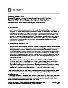
(horizontal) length is 487.62 meters. In the simulation, the branch eventually reaches equilibrium after an initial concentration is put in. A concentration of 3 g/m3 and of 100 g/m3 were tested for the model. The chosen diameter assessed for this study is 0.2 mm with a specific gravity of 1.8, found by Edinger (2002). The corresponding bottom sediment concentration is 3 mg/l or g/m3. The particle Reynolds number chosen for simulation is from Equation (41) because R is calculated to be between 6.61 and 282.84, but any of the equations can be used depending on the diameter and specific gravity of the particle. As previously stated, the horizontal and vertical water velocities, widths and bottom shear stresses for each cell are used in the simulation of the Spokane River. Vertical eddy viscosity can also be computed in the model, but the values are small enough that a general value is chosen for this model. Values are taken from the snapshot output (snp.opt) feature of CE-QUAL-W2 and only show values to the thousandth. Many vertical eddy viscosity values are less than this so to see an effect, the general value of 0.001 m2/s is used. Vertical eddy viscosity calculates the vertical mass turbulent diffusion coefficient (see Equation (39)). The horizontal mass turbulent diffusion coefficient is many magnitudes smaller than the vertical mass turbulent diffusion coefficient, as found by a non-dimensional ratio of the two values, and is neglected in this model. The value of the horizontal coefficient can be calculated by Equation (38) when the horizontal grid spacing is known and can be implemented in future models. When putting in an initial concentration of 100 g/m3, the profile looks like Figure 2, below after one day of simulation. The dimensionless height is the ratio of the height of the cell, z, to the height above the sea bed (water height from bed to surface). The profile of an initial concentration of 3 g/m3 has a very similar profile with different values as the sediment settles and moves around the system. When reviewing the work of van Rijn (1987), the tested profiles are similar to that of Figure 2. 0.9

Dimensionless Height, z/H

0.8 0.7 0.6 0.5 0.4 0.3 0.2 0.1 0 0

2

4

6

8

10

12

14

Sediment Concentration (g/m^3)

Figure 2: Sediment Concentration with Dimensionless Height above Sea Bed to Water Surface

15

The simulation is run for up to 60 days for this study. The value of concentration eventually settles down to a value in each cell that shows the relationship between velocity and the source/sink terms. This value of concentration becomes constant in each cell as time passes. Simulated times are at 1 day, 5 days, 10 days, 40 days and 60 days to show variation in concentration values. The CE-QUAL-W2 snapshot values are shown after 200 days of simulation and do not change throughout the time series for this study. When the sediment concentration equations are eventually converted to Fortran and run with the model, they will vary more as velocity varies throughout the simulation, which this model does not do. The concentration value is also a variable that will change the values throughout the system. The simulation produced a sufficient outcome to test the equations for sediment transport. There are small inaccuracies from averaging and neglecting data that should be taken into account when putting this transport equation into CE-QUAL-W2. The scour and fall velocity terms seem to counter each other in a way that accurately represents the forces acting on sediment in motion. Plots can be found in Appendix A that show depth versus concentration of the sediment in the branch. The depth value increases as it gets closer to the river bed. Note that the concentration of all the plots looks very similar and the numbers are decreasing with time. Tables can be found in Appendix B for the plot values.

4.0 Conclusions & Future Recommendations Sediment transport is a complex and extensive process. One-, two- and three-dimensional models can all simulate this process and can be used for different assessments of transport. Each model has either simplifying or complex qualities that make it the most efficient and precise model for the occasion. There is much more to be done to evaluate sediment and its course through a water body for CEQUAL-W2. Concentration of sediment is the first step to finding bed load, suspended load and total load. The equations presented in this study provide a base for laterally averaged sediment concentrations that can be implemented for a variety of flows and sediment characteristics. This study shows that the scour equation developed by Nielson (1992) and implemented by Edinger (2002) is sufficient to produce accurate results when simulating sediment transport. However, the modeler must be wary of the changes in the sediment transport process from certain equation variations, especially for different sediment characteristics. The simplifications in Section 3.0 must be taken into consideration when moving further with sediment transport modeling. Equations for all values that are needed and not yet calculated in CE-QUAL-W2 are shown in Section 2.0. There are certain equations that only a range of grain diameters fit in, such as the particle Reynolds number, evaluating the drag coefficient and particle velocity. These discrepancies create variations in transport of sediment. Once sediment concentration can be written into CE-QUAL-W2, further assessment of sediment transport representation can be developed.

16

5.0 References Cao, Z., Pender, G., and Meng, J. (2006) Explicit Formulation of the Shields Diagram for Incipient Motion of Sediment, ASCE, Journal of Hydraulic Engineering, October, 1097-1099, 10.1061/(ASCE)07339429(2006)132:10(1097). Coastal and Hydraulics Laboratory. U.S. Army Engineer Research and Development Center. Retrieved May 20, 2014 from http://chl.erdc.usace.army.mil/ Cole, T.M., and S.A. Wells (2014). “CE-QUAL-W2: A two-dimensional, laterally averaged, hydrodynamic and water quality model, version 3.71 user manual.” Portland State University. “Delft3D suite: 3D/2D modelling suite for integral water solutions” (2012). Deltares Systems. Retrieved May 20, 2014 from http://www.usbr.gov/pmts/sediment/model/srh2d/ Edinger, J. E. (2002) Waterbody Hydrodynamic and Water Quality Modeling, ASCE Press, Reston, Virginia. Hydrologic Engineering Center. “HEC-RAS.” U.S. Army Corps of Engineers. Retrieved May 25, 2014 from http://www.hec.usace.army.mil/software/hec-ras/ “Modelling the world of water: Software catalogue” (2011). MIKE by DHI. Nielson, P. (1992). “Coastal bottom boundary layers and sediment transport.” Volume 4. Advanced Series on Ocean Engineering, World Scientific Publishing Co. Ltd. River Edge, NJ. Simoes, F.J.M. and C.T. Yang (2006). “Chapter 5: Sediment modeling for rivers and reservoirs,” in Erosion and Sedimentation Manual. U.S. Department of the Interior, Bureau of Reclamation. Denver, CO. Symonds, A. (2012). “Sediment transport models,” in Stream and Watershed Restoration. Tangient LLC. San Francisco, CA. Technical service center: Sedimentation and river hydraulics group. “SRH-2D: Sedimentation and river hydraulics – two dimensional models.” U.S. Department of the Interior, Bureau of Reclamation. Retrieved May 4, 2014 from http://www.usbr.gov/pmts/sediment/model/srh2d/ U.S. Army Corps of Engineers (1989). “Engineering and design: Sedimentation and investigations of rivers and reservoirs.” Washington D.C. van Rijn, L.C. (1987). “Mathematical modeling of morphological processes in the case of suspended sediment transport.” Doctoral Thesis. Dept. of Fluid Mechanics, Delft Univ. of Technology, Delft, The Netherlands. Vieira, D.A., and Weiming Wu (2002). “CCHE1D version 3.0 – Model capabilities and applications.” National Center for Computational Hydroscience and Engineering. The University of Mississippi. Wagner, C.R. (2004). “Results of a two-dimensional hydrodynamic and sediment-transport model to predict the effects of the phased construction and operation of the Olmsted Locks and Dam on the Ohio River near Olmsted, Illinois.” U.S. Department of the Interior and U.S. Geological Survey. Louisville, KY. Whipple, K. (2004). “Surface processes and eandscape evolution: Essentials of sediment transport.” MIT OCW. Retrieved 2014-12-08. Wu W. (2002). “One-dimensional channel network model; CCHE1D – Technical Manual.” National Center for Computational Hydroscience and Engineering. Technical Report No. NCCHE-TR-2002-1 Yang, C.T. (1996). “Sediment Transport Theory and Practice.” The McGraw-Hill Companies, Inc.

17

APPENDIX A Sediment Concentration Plots

0.9

Dimensionless Height, z/H

0.8 0.7 0.6 0.5 0.4 0.3 0.2 0.1 0 0.000

0.050

0.100

0.150

0.200

0.250

0.300

0.350

0.400

0.450

Sediment Concentration (g/m^3) 2

Figure 3: Sediment Concentration at 1 Day of Simulation with 3 g/m of Initial Concentration

0.9

Dimensionless Height, z/H

0.8 0.7 0.6 0.5 0.4 0.3 0.2 0.1 0 0.000

0.010

0.020

0.030

0.040

0.050

0.060

Sediment Concentration (g/m^3) 2

Figure 4: Sediment Concentration at 5 Days of Simulation with 3 g/m of Initial Concentration

A-1

0.9

Dimensionless Height, z/H

0.8 0.7 0.6 0.5 0.4 0.3 0.2 0.1 0 0.000

0.005

0.010

0.015

0.020

Sediment Concentration (g/m^3) 2

Figure 5: Sediment Concentration at 10 Days of Simulation with 3 g/m of Initial Concentration

0.9

Dimensionless Height, z/H

0.8 0.7 0.6 0.5 0.4 0.3 0.2 0.1 0 0.0000 0.0020 0.0040 0.0060 0.0080 0.0100 0.0120 0.0140 0.0160 0.0180

Sediment Concentration (g/m^3) 2

Figure 6: Sediment Concentration at 40 Days of Simulation with 3 g/m of Initial Concentration

A-2

0.9

Dimensionless Height, z/H

0.8 0.7 0.6 0.5 0.4 0.3 0.2 0.1 0 0.0000 0.0020 0.0040 0.0060 0.0080 0.0100 0.0120 0.0140 0.0160 0.0180

Sediment Concentration (g/m^3) 2

Figure 7: Sediment Concentration at 60 Days of Simulation with 3 g/m of Initial Concentration

0.9

Dimensionless Height, z/H

0.8 0.7 0.6 0.5 0.4 0.3 0.2 0.1 0 0.000

2.000

4.000

6.000

8.000

10.000

12.000

14.000

Sediment Concentration (g/m^3) 2

Figure 8: Sediment Concentration at 1 Day of Simulation with 100 g/m of Initial Concentration

A-3

0.9

Dimensionless Height, z/H

0.8 0.7 0.6 0.5 0.4 0.3 0.2 0.1 0 0.000

0.200

0.400

0.600

0.800

1.000

1.200

1.400

Sediment Concentration (g/m^3) 2

Figure 9: Sediment Concentration at 5 Days of Simulation with 100 g/m of Initial Concentration

0.9

Dimensionless Height, z/H

0.8 0.7 0.6 0.5 0.4 0.3 0.2 0.1 0 0.000

0.010

0.020

0.030

0.040

0.050

0.060

0.070

0.080

0.090

Sediment Concentration (g/m^3) 2

Figure 10: Sediment Concentration at 10 Days of Simulation with 100 g/m of Initial Concentration

A-4

0.9

Dimensionless Height, z/H

0.8 0.7 0.6 0.5 0.4 0.3 0.2 0.1 0 0.0000 0.0020 0.0040 0.0060 0.0080 0.0100 0.0120 0.0140 0.0160 0.0180

Sediment Concentration (g/m^3) 2

Figure 11: Sediment Concentration at 40 Days of Simulation with 100 g/m of Initial Concentration

0.9

Dimensionless Height, z/H

0.8 0.7 0.6 0.5 0.4 0.3 0.2 0.1 0 0.0000 0.0020 0.0040 0.0060 0.0080 0.0100 0.0120 0.0140 0.0160 0.0180

Sediment Concentration (g/m^3) 2

Figure 12: Sediment Concentration at 60 Days of Simulation with 100 g/m of Initial Concentration

A-5

APPENDIX B Sediment Concentration Tables

2

Layer Number (depth, m)

Table 2: Sediment Concentration at 1 Day of Simulation with 3 g/m of Initial Concentration

0.57 1.4 1.9 2.4 2.9 3.4 3.9

2 0.248 0.370 0.382 0.403 0.427 0.455 0.457

3 0.238 0.361 0.373 0.374 0.376 0.388 0.387

Segment Number (length, m) 4 5 0.122 0.086 0.183 0.129 0.337 0.230 0.460 0.391 0.460 0.491 0.446 0.490 0.445 0.489

6 0.069 0.100 0.178 0.302 0.525 0.526 0.525

7 0.056 0.086 0.153 0.259 0.574 0.575 0.575

2

Layer Number (depth, m)

Table 3: Sediment Concentration at 5 Days of Simulation with 3 g/m of Initial Concentration

0.57 1.4 1.9 2.4 2.9 3.4 3.9

2 0.033 0.049 0.050 0.053 0.056 0.060 0.060

3 0.031 0.047 0.049 0.049 0.049 0.051 0.051

Segment Number (length, m) 4 5 0.016 0.011 0.024 0.017 0.044 0.030 0.060 0.051 0.060 0.065 0.059 0.064 0.058 0.064

6 0.009 0.013 0.023 0.040 0.069 0.069 0.069

7 0.007 0.011 0.020 0.034 0.075 0.076 0.075

2

Layer Number (depth, m)

Table 4: Sediment Concentration at 10 Days of Simulation with 3 g/m of Initial Concentration

0.57 1.4 1.9 2.4 2.9 3.4 3.9

2 0.011 0.017 0.017 0.018 0.019 0.021 0.021

3 0.011 0.016 0.017 0.017 0.017 0.018 0.017

Segment Number (length, m) 4 5 0.006 0.004 0.008 0.006 0.015 0.010 0.021 0.018 0.021 0.022 0.020 0.022 0.020 0.022

6 0.003 0.005 0.008 0.014 0.024 0.024 0.024

7 0.003 0.004 0.007 0.012 0.026 0.026 0.026

2

Layer Number (depth, m)

Table 5: Sediment Concentration at 40 Days of Simulation with 3 g/m of Initial Concentration

0.57 1.4 1.9 2.4 2.9 3.4 3.9

2 0.0100 0.0150 0.0154 0.0163 0.0173 0.0184 0.0185

3 0.0096 0.0146 0.0151 0.0151 0.0152 0.0157 0.0156

Segment Number (length, m) 4 5 0.0050 0.0035 0.0074 0.0052 0.0136 0.0093 0.0186 0.0158 0.0186 0.0199 0.0181 0.0198 0.0180 0.0198

B-1

6 0.0028 0.0041 0.0072 0.0122 0.0212 0.0213 0.0212

7 0.0023 0.0035 0.0062 0.0105 0.0232 0.0232 0.0232

2

Layer Number (depth, m)

Table 6: Sediment Concentration at 60 Days of Simulation with 3 g/m of Initial Concentration

0.57 1.4 1.9 2.4 2.9 3.4 3.9

2 0.0100 0.0150 0.0154 0.0163 0.0173 0.0184 0.0185

3 0.0096 0.0146 0.0151 0.0151 0.0152 0.0157 0.0156

Segment Number (length, m) 4 5 0.0050 0.0035 0.0074 0.0052 0.0136 0.0093 0.0186 0.0158 0.0186 0.0199 0.0181 0.0198 0.0180 0.0198

6 0.0028 0.0041 0.0072 0.0122 0.0212 0.0213 0.0212

7 0.0023 0.0035 0.0062 0.0105 0.0232 0.0232 0.0232

2

Layer Number (depth, m)

Table 7: Sediment Concentration at 1 Day of Simulation with 100 g/m of Initial Concentration

0.57 1.4 1.9 2.4 2.9 3.4 3.9

2 8.135 12.132 12.499 13.195 13.975 14.916 14.965

3 7.808 11.826 12.215 12.259 12.305 12.706 12.661

Segment Number (length, m) 4 5 4.008 2.824 6.010 4.239 11.034 7.527 15.053 12.817 15.080 16.090 14.619 16.041 14.588 16.006

6 2.266 3.291 5.819 9.877 17.210 17.227 17.202

7 1.823 2.821 4.998 8.493 18.786 18.848 18.837

2

Layer Number (depth, m)

Table 8: Sediment Concentration at 5 Days of Simulation with 100 g/m of Initial Concentration

0.57 1.4 1.9 2.4 2.9 3.4 3.9

2 0.780 1.163 1.198 1.264 1.339 1.429 1.434

3 0.748 1.133 1.171 1.175 1.179 1.218 1.213

Segment Number (length, m) 4 5 0.384 0.271 0.576 0.406 1.057 0.721 1.442 1.228 1.445 1.542 1.401 1.537 1.398 1.534

6 0.217 0.315 0.558 0.946 1.649 1.651 1.648

7 0.175 0.270 0.479 0.814 1.800 1.806 1.805

2

Layer Number (depth, m)

Table 9: Sediment Concentration at 10 Days of Simulation with 100 g/m of Initial Concentration

0.57 1.4 1.9 2.4 2.9 3.4 3.9

2 0.050 0.075 0.078 0.082 0.087 0.093 0.093

3 0.048 0.073 0.076 0.076 0.076 0.079 0.079

Segment Number (length, m) 4 5 0.025 0.018 0.037 0.026 0.068 0.047 0.093 0.080 0.094 0.100 0.091 0.100 0.091 0.099

B-2

6 0.014 0.020 0.036 0.061 0.107 0.107 0.107

7 0.011 0.018 0.031 0.053 0.117 0.117 0.117

2

Layer Number (depth, m)

Table 10: Sediment Concentration at 40 Days of Simulation with 100 g/m of Initial Concentration

0.57 1.4 1.9 2.4 2.9 3.4 3.9

2 0.0100 0.0150 0.0154 0.0163 0.0173 0.0184 0.0185

3 0.0096 0.0146 0.0151 0.0151 0.0152 0.0157 0.0156

Segment Number (length, m) 4 5 0.0050 0.0035 0.0074 0.0052 0.0136 0.0093 0.0186 0.0158 0.0186 0.0199 0.0181 0.0198 0.0180 0.0198

6 0.0028 0.0041 0.0072 0.0122 0.0212 0.0213 0.0212

7 0.0023 0.0035 0.0062 0.0105 0.0232 0.0232 0.0232

2

Layer Number (depth, m)

Table 11: Sediment Concentration at 60 Days of Simulation with 100 g/m of Initial Concentration

0.57 1.4 1.9 2.4 2.9 3.4 3.9

2 0.0100 0.0150 0.0154 0.0163 0.0173 0.0184 0.0185

3 0.0096 0.0146 0.0151 0.0151 0.0152 0.0157 0.0156

Segment Number (length, m) 4 5 0.0050 0.0035 0.0074 0.0052 0.0136 0.0093 0.0186 0.0158 0.0186 0.0199 0.0181 0.0198 0.0180 0.0198

B-3

6 0.0028 0.0041 0.0072 0.0122 0.0212 0.0213 0.0212

7 0.0023 0.0035 0.0062 0.0105 0.0232 0.0232 0.0232

APPENDIX C Upwind Center Space Scheme Matlab Code for Sediment Concentration

%% Upwind Center Space Scheme for Sediment Concentration delz=0.5; % grid spacing in meters in z direction delt=5; % delta t in seconds, chosen by W2 model tottime=(3600*24); % time of evaluation or total time for evaluation. Change 24 hours to change time k=7; % number of layers i=6; % number of segments % grid spacing in x direction (m) – from W2 – constant value %delx(1,1:i)=[487.620,487.620,487.620,487.620,487.620,487.620]; %delx(2,1:i)=[487.620,487.620,487.620,487.620,487.620,487.620]; %delx(3,1:i)=[487.620,487.620,487.620,487.620,487.620,487.620]; %delx(4,1:i)=[487.620,487.620,487.620,487.620,487.620,487.620]; %delx(5,1:i)=[487.620,487.620,487.620,487.620,487.620,487.620]; %delx(6,1:i)=[487.620,487.620,487.620,487.620,487.620,487.620]; %delx(7,1:i)=[487.620,487.620,487.620,487.620,487.620,487.620]; %delx(8,1:i)=[487.620,487.620,487.620,487.620,487.620,487.620]; delx=487.620; % grid spacing in meters in x direction % Horizontal velocity profile, U (m/s) – from W2 U(1,1:i)=[2.367,2.669,2.212,1.950,1.787,3.638]; U(2,1:i)=[2.301,2.325,1.939,1.761,1.629,1.496]; U(3,1:i)=[2.301,2.462,1.966,1.753,1.628,1.489]; U(4,1:i)=[2.301,2.594,2.124,1.768,1.552,1.394]; U(5,1:i)=[2.301,2.594,2.201,1.946,1.772,1.604]; U(6,1:i)=[2.300,2.594,2.201,1.946,1.772,1.604]; U(7,1:i)=[1.015,1.309,1.201,1.162,1.128,1.052]; % Vertical velocity profile, W (m/s) from W2 W(1,1:i)=[0.008,0.003,0.001,0.001,0.000,0.000]; W(2,1:i)=[0.007,0.002,-0.000,0.000,0.000,-0.000]; W(3,1:i)=[0.006,0.001,-0.001,-0.000,0.000,-0.000]; W(4,1:i)=[0.004,0.001,-0.001,-0.000,-0.000,-0.000]; W(5,1:i)=[0.002,0.001,-0.001,-0.000,-0.000,-0.000]; W(6,1:i)=[0.000,0.000,-0.000,-0.000,-0.000,-0.000]; W(7,1:i)=[0.000,0.000,0.000,0.000,0.000,0.000]; % Vertical Eddy Viscosity, Az (to calculate Dz) (m^2/s) from W2 – not used %Az(1,1:i)=[0.000,0.000,0.000,0.000,0.000,0.000]; %Az(2,1:i)=[0.000,0.000,0.000,0.000,0.000,0.000];

C-1

%Az(3,1:i)=[0.000,0.000,0.000,0.000,0.000,0.000]; %Az(4,1:i)=[0.000,0.000,0.000,0.000,0.000,0.000]; %Az(5,1:i)=[0.000,0.000,0.000,0.000,0.000,0.000]; %Az(6,1:i)=[0.000,0.000,0.000,0.000,0.000,0.000]; %Az(7,1:i)=[0.000,0.000,0.000,0.000,0.000,0.000]; Az=0.001; % Bottom shear stress, taub (m^3/s^2) from W2 tb(1,1:i)=[4.973,5.596,5.234,4.565,4.316,3.696]; tb(2,1:i)=[0.325,1.500,2.636,2.832,2.957,2.861]; tb(3,1:i)=[0.325,0.722,1.375,1.653,1.686,1.630]; tb(4,1:i)=[0.325,0.324,0.473,0.919,1.368,1.490]; tb(5,1:i)=[0.325,0.324,0.252,0.198,0.163,0.139]; tb(6,1:i)=[0.325,0.324,0.252,0.198,0.163,0.139]; tb(7,1:i)=[3.539,3.537,2.753,2.159,1.774,1.517]; % Width of each segment, B (m) B(1:k,1)=[7.30000,5.00000,5.00000,5.00000,5.00000,5.00000,5.00000]; B(1:k,2)=[7.30000,5.00000,5.00000,5.00000,5.00000,5.00000,5.00000]; B(1:k,3)=[17.4000,12.0000,6.80000,5.00000,5.00000,5.00000,5.00000]; B(1:k,4)=[27.5000,18.9000,10.7000,6.30000,5.00000,5.00000,5.00000]; B(1:k,5)=[37.6000,25.9000,14.7000,8.70000,5.00000,5.00000,5.00000]; B(1:k,6)=[47.7000,32.8000,18.6000,11.0000,5.00000,5.00000,5.00000]; Ci=100; % Boundary condition, sediment conc coming into system, g/m^3 – either 100 or 3 Co=0; % BC for sed concentration above the bed at upstream boundary. This may gradually decrease from 100 or 3 instead of start at 0 in a real model Dx=0; % m^2/sec % Dx=(5.84*10.^-4)*(delx.^1.1) but it is neglected due to Dz having a significantly larger magnitude and snapshot only allowing 3 decimal points which makes Az=0 more than it should. Dz=0.14*Az; nts=tottime/delt; % number time steps ndx=i; % number of grid points in x direction ndz=k; % number of grid points in y direction % Explicit Upwind CS (FTBSCS) %C^n Amat(ndz,ndx)=0; Amat(ndz,1)=Ci; % Boundary condition

C-2

% definitions: % B=B(K,I); % U=U(K,I); % W=W(K,I); % Dz=0.14*Az(K,I); % delx=delx(K,I); g=9.8; % acceleration due to gravity, m/s^2 d=(2*10.^-4); % sediment particle diameter, m Sg=1.8; % specific gravity defined for particle with diameter d1 Cb=3; % min bottom conc. for d1 and Sg1 (to compute Cbottom of source term), g/m^3 % Cb can also be found experimentally with Cbottom=Ckb*exp(Ws*delz/(0,14Az(K,I)); where Ckb is known bottom concentration of suspended solids (mg/l or g/m^3) rhow=998777; % density of water, g/m^3 (this may vary with different water, use W2 values) rhos=Sg*rhow; % density of sediment particle d, g/m^3 T=17; % temperature, degrees celcius v=(1.79*10.^-6)*exp(-0.0266*T); % kinematic viscosity R=d*sqrt(Sg*g*d)/v; % R is less than 6.6, so can use 0.1414R.^0.2306 for critical Shield's Tc=(((1+((0.0223*R).^2.8358)).^0.3542)/(3.0946*R.^0.6769)); % critical Shield's number for R between 6.6 and 282.8 % T= (tb(K,I)/(g*(Sg-1)*d)) ; % must be in equation because tb changes Cd=24/R; % drag coefficient, should be found experimentally when R>2.0 Ws2=sqrt((4*g*(Sg2-1)*d2)/(3*Cd2)); % settling velocity of particle with d2 % for sediment with diameter d2, only branch 1 % B Matrix for C^n+1, C^n+2, C^n+3, etc. for t=[0:delt:tottime]; for K=[ndz:-1:1]; for I=[1:ndx]; if K==1 & I==1; Bmat(K,I)=(delt/B(K,I))*((Dx*((B(K,I)+B(K,I+1))/2)*((Amat(K,I+1)Amat(K,I))/delx))-(Dx*((B(K,I)+B(K,I+1))/2)*((Amat(K,I)Amat(K,I+1))/delx))+(Dz*((B(K,I)+B(K+1,I))/2)*((Amat(K+1,I)-Amat(K,I))/delz))(Dz*((B(K,I)+B(K+1,I))/2)*((Amat(K+1,I)-Amat(K,I))/delz))-(B(K,I)*((((0.00033*(((tb(K,I)/(g*(rhosrhow)*d))/Tc)-1)*((Sg-1).^0.6)*(g.^0.6)*(d.^0.8))/(v.^0.2))*Cb)/delx))-(Ws*(((B(K,I)*Amat(K,I))(B(K+1,I)*Amat(K+1,I)))/delz))-(((U(K,I)*B(K,I)*Amat(K,I))-(U(K,I+1)*B(K,I+1)*Amat(K,I+1)))/delx)(((W(K,I)*B(K,I)*Amat(K,I))-(W(K+1,I)*B(K+1,I)*Amat(K+1,I)))/delz))+Amat(K,I); elseif K==ndz & I==1; Bmat(K,I)=(delt/B(K,I))*((Dx*((B(K,I)+B(K,I+1))/2)*((Amat(K,I+1)Amat(K,I))/delx))-(Dx*((B(K,I)+B(K,I+1))/2)*((Amat(K,I)-Amat(K,I+1))/delx))+(Dz*((B(K,I)+B(K1,I))/2)*((Amat(K-1,I)-Amat(K,I))/delz))-(Dz*((B(K,I)+B(K-1,I))/2)*((Amat(K-1,I)-Amat(K,I))/delz))-

C-3

(B(K,I)*((((0.00033*(((tb(K,I)/(g*(rhos-rhow)*d))/Tc)-1)*((Sg1).^0.6)*(g.^0.6)*(d.^0.8))/(v.^0.2))*Cb)/delx))-(Ws*(((B(K,I)*Amat(K,I))-(B(K-1,I)*Amat(K-1,I)))/delz))(((U(K,I)*B(K,I)*Amat(K,I))-(U(K,I+1)*B(K,I+1)*Amat(K,I+1)))/delx)-(((W(K,I)*B(K,I)*Amat(K,I))-(W(K1,I)*B(K-1,I)*Amat(K-1,I)))/delz))+Amat(K,I); elseif K==1 & I==ndx; Bmat(K,I)=(delt/B(K,I))*((Dx*((B(K,I)+B(K,I-1))/2)*((Amat(K,I-1)-Amat(K,I))/delx))(Dx*((B(K,I)+B(K,I-1))/2)*((Amat(K,I)-Amat(K,I-1))/delx))+(Dz*((B(K,I)+B(K+1,I))/2)*((Amat(K+1,I)Amat(K,I))/delz))-(Dz*((B(K,I)+B(K+1,I))/2)*((Amat(K+1,I)-Amat(K,I))/delz))(B(K,I)*((((0.00033*(((tb(K,I)/(g*(rhos-rhow)*d))/Tc)-1)*((Sg1).^0.6)*(g.^0.6)*(d.^0.8))/(v.^0.2))*Cb)/delx))-(Ws*(((B(K,I)*Amat(K,I))-(B(K+1,I)*Amat(K+1,I)))/delz))(((U(K,I)*B(K,I)*Amat(K,I))-(U(K,I-1)*B(K,I-1)*Amat(K,I-1)))/delx)-(((W(K,I)*B(K,I)*Amat(K,I))(W(K+1,I)*B(K+1,I)*Amat(K+1,I)))/delz))+Amat(K,I); elseif K==ndz & I==ndx; Bmat(K,I)=(delt/B(K,I))*((Dx*((B(K,I)+B(K,I-1))/2)*((Amat(K,I-1)-Amat(K,I))/delx))(Dx*((B(K,I)+B(K,I-1))/2)*((Amat(K,I)-Amat(K,I-1))/delx))+(Dz*((B(K,I)+B(K-1,I))/2)*((Amat(K-1,I)Amat(K,I))/delz))-(Dz*((B(K,I)+B(K-1,I))/2)*((Amat(K-1,I)-Amat(K,I))/delz))(B(K,I)*((((0.00033*(((tb(K,I)/(g*(rhos-rhow)*d))/Tc)-1)*((Sg1).^0.6)*(g.^0.6)*(d.^0.8))/(v.^0.2))*Cb)/delx))-(Ws*(((B(K,I)*Amat(K,I))-(B(K-1,I)*Amat(K-1,I)))/delz))(((U(K,I)*B(K,I)*Amat(K,I))-(U(K,I-1)*B(K,I-1)*Amat(K,I-1)))/delx)-(((W(K,I)*B(K,I)*Amat(K,I))-(W(K1,I)*B(K-1,I)*Amat(K-1,I)))/delz))+Amat(K,I); elseif K>1 & K1 & K1 & I1 & I