Published in: E. Kurz-Milcke & G. Gigerenzer (Eds.), Experts in science and society (pp. 249–268). © 2004 Kluwer Academic/Plenum Publisher.
How to Improve the Diagnostic Inferences of Medical Experts Ulrich Hoffrage and Gerd Gigerenzer Center for Adaptive Behavior and Cognition Max Planck Institute for Human Development, Berlin, Germany
Women are generally informed that mammography screening reduces the risk of dying from breast cancer by 25%. Does that mean that from 100 women who participate in screening, 25 lives will be saved? Although many people believe this to be the case, the conclusion is not justified. This figure means that from 1,000 women who participate in screening, 3 will die from breast cancer within 10 years, whereas from 1,000 women who do not participate, 4 will die. The difference between 4 and 3 is the 25% “relative risk reduction.” Expressed as an “absolute risk reduction,” however, this means that the benefit is 1 in 1,000, that is, 0.1%. Cancer organizations and health departments continue to inform women of the relative risk reduction, which gives a higher number—25% as compared to 0.1%—and makes the benefit of screening appear larger than if it were represented in absolute risks. The topic of this chapter is the representation of information on medical risks. As the case of mammography screening illustrates, the same information can be presented in various ways. The general point is that information always requires representation, and the choice between alternative representations can influence the patients’ willingness to participate in screening, or more generally, patients’ understanding of risks and choices of medical treatments. The ideal of “informed consent” can only be achieved if the patient knows about the pros and cons of a treatment, or the chances that a particular diagnosis is right or wrong. However, in order to communicate such uncertainties to the patients, the physician has to first understand statistical information and its implications. This requirement sharply contrasts with the fact that physicians are rarely trained in risk communication, and some still think that medicine can dispense with statistics and psychology. Such reluctance may also explain why previous research observed that a majority of physicians do not use relevant statistical information properly in diagnostic inference. Casscells, Schoenberger, and Grayboys (1978), for instance, asked 60 house officers, students, and physicians at the Harvard Medical School to estimate the probability of an unnamed disease given the following information: If a test to detect a disease whose prevalence is 1/1,000 has a false positive rate of 5 per cent, what is the chance that a person found to have a positive result actually has the disease, assuming that you know nothing about the person’s symptoms or signs? (p. 999)
The estimates varied wildly, from the most frequent estimate, 95% (27 out of 60), down to 2% (11 out of 60). The value of 2% is obtained by inserting the problem information into Bayes’ rule (see below)—assuming that the sensitivity of the test, which is not specified in the problem, is approximately 100%. Casscells et al. (1978) concluded that “(...) in this group of students and physicians, formal decision analysis was almost entirely unknown and even common-sense reasoning about the interpretation of laboratory data was uncommon” (p. 1000).
2
How to Improve the Diagnostic Inferences of Medical Experts
In a seminal article on probabilistic reasoning about mammography, David Eddy (1982) reported an informal study in which he asked an unspecified group of physicians to estimate the probability of breast cancer given a base rate (prevalence) of 1%, a hit rate (sensitivity) of 79%, and a false positive rate of 9.6%. He reported that 95 out of 100 physicians gave estimates of the posterior probability of breast cancer given a positive mammogram (the positive predictive value) of between 70% and 80%, whereas Bayes’ rule results in a value one order of magnitude smaller, namely, 7.7%. Eddy proposed that the majority of physicians confused the sensitivity of the test with the positive predictive value. Evidence of this confusion can also be found in medical textbooks and journal articles (Eddy, 1982), as well as in statistical textbooks (Gigerenzer, 1993). In 1986, Windeler and Köbberling reported responses to a questionnaire they had mailed to family physicians, surgeons, internists, and gynecologists in Germany. Only 13 of the 50 respondents realized that an increase in a disease’s prevalence implies an increase in the positive predictive value. The authors concluded with this puzzling observation: Although intuitive judgment of probabilities is part of every diagnostic and treatment decision, the physicians in their study were obviously unaccustomed to estimating quantitative probabilities. Given these demonstrations that many physicians’ reasoning does not follow the laws of probability (see also Abernathy & Hamm, 1995; Dawes, 1988; Dowie & Elstein, 1988), what can be done to improve diagnostic inference?
Natural Frequencies Help in Making Diagnostic Inferences Each of the three studies summarized above presented numerical information in the form of probabilities and percentages. The same holds for other studies in which the conclusion was that physicians (Berwick, Fineberg, & Weinstein, 1981; Politser, 1984) and laypeople (Koehler, 1996a) have great difficulties in making diagnostic inferences from statistical information. Whether information is presented in probabilities, percentages, absolute frequencies, or some other form is irrelevant from a mathematical viewpoint. These different representations can be mapped onto one another in a one-to-one fashion. However, they are not equivalent from a psychological viewpoint, which is the key to our argument. We argue that a specific class of representations, which we call natural frequencies, helps laypeople and experts to make inferences the Bayesian way. We illustrate the difference between probabilities and natural frequencies with the diagnostic problem of inferring the presence of colorectal cancer (C) from a positive result in the hemoccult test (T), a standard diagnostic test. In terms of probabilities, the relevant information is a base rate for colorectal cancer p(C) = 0.3%, a sensitivity p(T |C) = 50%, and a false positive rate p(T | not-C) = 3%. In natural frequencies, the same information would read: Thirty out of every 10,000 people have colorectal cancer. Of these 30 people with colorectal cancer, 15 will have a positive hemoccult test. Of the remaining 9,970 people without colorectal cancer, 300 will still have a positive hemoccult test.
Natural frequencies are absolute frequencies as encoded through direct experience and have not been normalized with respect to the base rates of disease and non-disease (Gigerenzer & Hoffrage, 1995, 1999). They are to be distinguished from probabilities, percentages, relative frequencies, and other representations where the underlying natural frequencies have been normalized with respect to these base rates.1 Why should natural frequencies facilitate diagnostic inferences? There are two related arguments. The first is computational. Bayesian computations are simpler when the information is
Ulrich Hoffrage and Gerd Gigerenzer
3
represented in natural frequencies rather than in probabilities, percentages, or relative frequencies (Christensen-Szalanski & Bushyhead, 1981; Kleiter, 1994). For instance, when the information concerning colorectal cancer is represented in probabilities, applying a cognitive algorithm to compute the positive predictive value, that is, the Bayesian posterior probability, amounts to performing the following computation: p(C ) p(T C ) ( .003 ) ( .5 ) p ( C T ) = ----------------------------------------------------------------------------------------- = ----------------------------------------------------------p ( C ) p ( T C ) + p ( not-C ) p ( T not-C ) ( .003 ) ( .5 ) + ( .997 ) ( .03 )
(1)
The result is 0.048. Equation 1 is Bayes’ rule for binary hypotheses (here, C and not-C) and data (here, T). The rule is named after Thomas Bayes (1702–1761), an English dissident minister, to whom the solution of the problem of how to make an inference from data to hypothesis is attributed (Stigler, 1983). When the information is presented in natural frequencies, then the computations are much simpler: c&t 15 p ( C T ) = ---------------------------------- = --------------------c&t + not-c&t 15 + 300
(2)
Equation 2 is Bayes’ rule for natural frequencies, where c&t is the number of cases with cancer and a positive test, and not-c&t is the number of cases without cancer but with a positive test. The second argument supplements the first. Minds appear to be tuned to make inferences from natural frequencies rather than from probabilities and percentages. This argument is consistent with developmental studies indicating the primacy of reasoning with discrete numbers over fractions, and studies of adult humans and animals indicating the ability to monitor frequency information in natural environments in fairly accurate and automatic ways (e.g., Gallistel & Gelman, 1992; Jonides & Jones, 1992; Real, 1991; Sedlmeier, Hertwig, & Gigerenzer, 1998). For most of their existence, humans and animals have made inferences from information encoded sequentially through direct experience, and natural frequencies are the final tally of such a process. Mathematical probability emerged only in the mid-17th century (Daston, 1988), and not until the aftermath of the French Revolution—when the metric system was adopted—do percentages appear to have become common representations, mainly for taxes and interests, and only very recently for risk and uncertainty (Gigerenzer et al., 1989). Thus, one might speculate that minds have evolved to deal with natural frequencies rather than with probabilities. Probabilities can be represented in what Gigerenzer and Hoffrage (1995) called the standard menu and the short menu. The standard menu is illustrated above; the short menu presents p(C&T) and p(T). Both lead to the same result. Similarly, natural frequencies can be expressed in both a standard and a short menu (see Appendix for all four versions of the colorectal cancer problem). To compute the Bayesian solution for probabilities, the short menu demands fewer computations than the standard menu, whereas for natural frequencies the computations are the 1
For instance, the following representation of the colorectal cancer problem is not in terms of natural frequencies (or frequency formats; Gigerenzer & Hoffrage, 1995, 1999), because the frequencies have been normalized with respect to the base rates: a base rate of 30 out of 10,000, a sensitivity of 5,000 out of 10,000, and a false positive rate of 300 out of 10,000.
4
How to Improve the Diagnostic Inferences of Medical Experts
same, except that in the standard menu the two compounds c&t and not-c&t need to be added to determine the denominator (Gigerenzer & Hoffrage, 1995, theoretical results 5 and 6, p. 688).
Do Natural Frequencies Improve Laypeople’s Reasoning? Many studies have concluded that people’s judgments do not follow Bayes’ rule, but little is known about how to help people reason the Bayesian way. We tested whether natural frequencies improve Bayesian inference in laypeople, specifically, students in various fields at the University of Salzburg (Gigerenzer & Hoffrage, 1995). We used 15 problems, including Eddy’s mammography problem and Tversky and Kahneman’s (1982) cab problem. When the information was presented in natural frequencies rather than in probabilities, the proportion of Bayesian responses increased systematically for each of the 15 problems. This advantage held whether the frequencies and probabilities were presented in the standard menu or the short menu. The average proportions of Bayesian responses were 16% and 28% for probabilities, rising to 46% and 50% for natural frequencies (standard and short menu, respectively). Thus, although they can be directly inserted in Equation 2, compound probabilities as displayed in the short menu were not as effective as natural frequencies. To conclude, natural frequencies, whether presented in the standard or the short menu, improve Bayesian reasoning without instruction. Similarly, Cosmides and Tooby (1996) showed that natural frequencies improve Bayesian inferences in the Casscell et al.’s (1978) problem as well. This hypothetical medical problem is numerically simpler (the hit rate is assumed to be 100%) than the problems in the Gigerenzer and Hoffrage (1995) study, and Cosmides and Tooby reported that 76% of the answers were Bayesian (see also Christensen-Szalanski & Beach, 1982). But would medical experts also profit from natural frequencies, and do they use them in communicating risks to their clients? The following studies with medical students and experienced physicians provide an answer to the first question; the final study with AIDS counselors addresses the second question.
Do Natural Frequencies Improve Medical Students’ Diagnostic Inferences? Participants were 87 advanced medical students of whom most had already passed a course in biostatistics and were, on average, in their fifth year, and 9 first-year interns. Fifty-four studied in Berlin and 42 in Heidelberg; 52 were female and 44 were male. The average age was 25 years. We chose four realistic diagnostic tasks and constructed four versions of each: two in which the information was presented in probabilities (as it typically is), and two in which the information was presented in natural frequencies. For each of these two formats the information was presented either in the standard menu or in the short menu. The four diagnostic tasks were to infer (a) the presence of colorectal cancer from a positive hemoccult test, (b) the presence of breast cancer from a positive mammogram, (c) the presence of phenylketonuria from a positive Guthrie test, and (d) the presence of ankylosing spondylitis (Bekhterev’s disease) from a positive HL-Antigen-B27 (HLA-B27) test. The information on prevalence (base rate), sensitivity (hit rate), and false positives (false-alarm rate) was taken from Eddy (1982), Mandel et al. (1993), Marshall (1993), Politser (1984), and Windeler and Köbberling (1986). The four diagnostic tasks are shown in the Appendix.
Ulrich Hoffrage and Gerd Gigerenzer
5
Percentage of Bayesian inferences
100 Probabilities, standard menu Probabilities, short menu Natural frequencies, standard menu Natural frequencies, short menu 75
50
25
0 Colorectal cancer
Breast cancer
Ankylosing spondylitis
Phenylketonuria
Overall
Figure 1. Medical students’ percentage of Bayesian inferences in four diagnostic tasks, broken down according to the four versions of each task (see Appendix for the four versions of the colorectal cancer problem).
These problems were given to the participants in a questionnaire. We used a Latin square design: Each participant worked on all problems, each in a different version. Across all participants, the four problems and the four versions appeared on each of the four pages in the questionnaire equally often. The first two problems in each questionnaire were always given in the same format, either both in probabilities or both in natural frequencies. In addition, we systematically varied the order of the two pieces of information in the short menu. Participants were paid a flat fee. They worked on the questionnaire at their own pace and in small groups of mainly three to six participants. The experimenter asked them to make notes, calculations, or drawings, so that we could reconstruct their reasoning. Interviews were performed after the participants completed their questionnaire. When a participant’s estimate was within plus or minus 5 percentage points (or the equivalent in frequencies) of the Bayesian estimate, and the notes and interview indicated that the estimate was arrived at by Bayesian reasoning (or a shortcut thereof; see Gigerenzer & Hoffrage, 1995) rather than by guessing or other means, then we classified the response as a “Bayesian inference.” Figure 1 shows the percentages of Bayesian inferences for the four diagnostic tasks (the results for the standard menu have already been published in Hoffrage, Lindsey, Hertwig, & Gigerenzer, 2000). For each problem, probabilities in the standard menu made it most difficult for the medical students to reason the Bayesian way. When the standard menu was used with natural frequencies, the performance increased from 18% to 57%. For the short menu, the differences were smaller, from 50% to 68%. This interaction is consistent with the theoretical result mentioned above—that the beneficial effect of the short menu is larger for probabilities than for natural frequencies. To summarize, medical students showed signs of “innumeracy” (Paulos, 1988) similar to those of laypeople when the information was in terms of probabilities (standard menu), but
6
How to Improve the Diagnostic Inferences of Medical Experts
their reasoning improved more than laypeople’s when the frequency representations (or probabilities in the short menu) were used.
Do Natural Frequencies Improve Physicians’ Diagnostic Inferences? As important as this result is for improving medical students’ “insight,” one might suspect that it will not generalize to experienced physicians who treat real patients. We asked 51 physicians to participate in the following study (Gigerenzer, 1996; Hoffrage & Gigerenzer, 1998). Three physicians did not give numerical estimates, either because they generally rejected statistical information as meaningless for medical diagnosis, or because they stated that they were unable to think in numbers. The remaining 48 physicians had practiced for an average of 14 years (ranging from 1 month to 32 years) and had a mean age of 42 years (ranging from 26 to 59). They worked either in Munich or Düsseldorf; 18 were female and 30 were male. Eighteen worked in university hospitals, 16 in private or public hospitals, and 14 in private practice. The sample included internists, gynecologists, dermatologists, and radiologists, among others. The physicians’ status ranged from directors of clinics to physicians commencing their careers. The interviewer visited the physicians individually at their institutions or private offices and, in a few cases, in their homes. She first informed the physician about our interest in studying diagnostic inference and established a relaxed personal rapport. Each physician was then given the same four diagnostic tasks as in the previous study. Each problem was printed on a sheet of paper, followed by a separate blank sheet. The interviewer asked the physician to use the empty sheet to make notes, calculations, or drawings so that we could later reconstruct his or her reasoning. After the physician completed the four tasks, the interviewer reviewed the physician’s notes. If it could not be discerned how the estimate was achieved in each task, the physician was asked for clarification. Given the limited free time of practicing physicians, we only used the standard menu. In two diagnostic tasks, the information was presented in probabilities, in the other two in natural frequencies. We systematically varied which tasks were in which format and which format was presented first with the constraint that the first two tasks had the same format.
Dr. Average To give the reader a better understanding of the test situation and the results, we first describe the results for Dr. Average, who represents the “average physician” with respect to performance on these diagnostic tasks. Dr. Average is a 59-year-old director of a university clinic who is active in research and teaching, a dermatologist with 32 years of professional experience. He worked on the problems for 30 minutes and spent another 15 minutes discussing the results with the interviewer. He was visibly nervous when working on the first two problems, which used probabilities. Initially, Dr. Average refused to make notes; he acquiesced later, when the interviewer again requested that he do so, but he did not let the interviewer see his notes. Dr. Average first worked on the mammography problem in the probability format. He calculated the probability of breast cancer after a positive mammography to be 90%, by adding the sensitivity to the false positive rate, 80% + 10% = 90%. Nervously, he remarked, “Oh, what nonsense. I can’t do it. You should test my daughter; she studies medicine.”
Ulrich Hoffrage and Gerd Gigerenzer
7
The second problem was on ankylosing spondylitis, also in the probability format. Dr. Average first commented that he himself had performed the HLA-B27 test (unlike the mammography test). Then he began to draw and calculate on his sheet of paper and remarked that the prevalence of 5% would be irrelevant. With some hesitation and annoyance, he estimated the probability of ankylosing spondylitis after a positive test to be 0.46%, by multiplying the sensitivity (92%) by the prevalence (5%). Apart from a calculation error by factor 10, this is a common strategy among laypeople (Gigerenzer & Hoffrage, 1995). The third problem was to diagnose colorectal cancer from a positive hemoccult test. The information was presented in natural frequencies. Dr. Average remarked, “But that’s so easy,” and calculated that 15 out of 315 people with a positive test would have colorectal cancer. This was the Bayesian answer. Unlike in the first two diagnostic inferences, he now seemed to realize that he had found the correct solution. His nervousness subsided. The phenylketonuria problem in natural frequencies came last. Dr. Average calculated that 10 out of 60 newborns with a positive Guthrie test have phenylketonuria, which again was the Bayesian answer. He said he had never advised parents on how to interpret a positive Guthrie test, whereas he had advised people on how to interpret a positive hemoccult test. During the following interview, Dr. Average discussed his strategies for estimating the predictive values of the tests with the interviewer, asked her to calculate the estimate for the mammography problem for him, and concluded, “That was fun.” Note that this physician’s performance was independent of whether he had experience with the specific test or not. What made the difference was whether the problem information was communicated in natural frequencies or probabilities. We now report the results aggregated across all physicians.
Forty-Eight Physicians Each of the 48 physicians made four diagnostic inferences. Thus, we have 48 estimates for each problem, and 24 estimates for each format of each problem. To classify a strategy as Bayesian, we used the same criteria as in the previous study. Figure 2 shows that for each diagnostic problem, the physicians reasoned the Bayesian way more often when the information was communicated in natural frequencies than in probabilities. The effect varied between problems, but even in the problem showing the weakest effect (phenylketonuria), the proportion of Bayesian answers was twice as large. For the two cancer problems, natural frequencies increased Bayesian inferences by more than a factor of five as compared to probabilities. Across all problems, the physicians gave the Bayesian answer with probabilities in only 10% of the cases; with natural frequencies this value increased to 46%. With probabilities, physicians spent an average of 25% more time solving the diagnostic problems than with natural frequencies. Moreover, physicians commented that they were nervous, tense, and uncertain more often when working with probabilities than with natural frequencies. They also stated that they were less skeptical of the relevance of statistical information when it was in natural frequencies. Physicians were conscious of their better and faster performance with natural frequencies, as illustrated by comments such as “Now it’s different. It’s quite easy to imagine. There is a frequency; that’s more visual” and “A first grader could do this!”
8
How to Improve the Diagnostic Inferences of Medical Experts
Percentage of Bayesian inferences
100 Probabilities Natural frequencies
50
25
0 Colorectal cancer
Breast cancer
Ankylosing spondylitis
Phenylketonuria
Overall
Figure 2. Physicians’ percentage of Bayesian inferences in the four diagnostic tasks, broken down according to whether the information was presented in probabilities or natural frequencies (in the standard menu only).
Innumeracy We asked the physicians how often they took statistical information into account when they interpreted the results of diagnostic tests. Twenty-six answered “very seldom or never,” 15 answered “once in a while,” 5 said “frequently,” and none answered “always.” Their comments suggested two reasons why physicians used statistical information rather infrequently: the physician’s innumeracy and the patient’s uniqueness. Several physicians perceived themselves as mathematically illiterate or suffering from a cognitive disease known as “innumeracy” (Paulos, 1988). Six physicians explicitly remarked on their inability to deal with numbers, stating, for instance, “But this is mathematics. I can’t do that. I’m too stupid for this.” With natural frequencies, however, these same physicians spontaneously reasoned statistically (i.e., in accordance with Bayes’ rule) as often as their peers who did not complain of innumeracy. Innumeracy and individual uniqueness were also the reasons why three physicians refused to complete our questionnaire. A 60-year-old high-ranking physician in a government agency wanted to give up on the first problem: “I simply can’t do that. Mathematics is not my forte.” When the interviewer encouraged her to try again, she tried, failed again, cursed loudly, and gave up. A second physician said: “I can’t do much with numbers. I am an intuitive being. I treat my patients in a holistic manner and don’t use statistics.” Finally, a university professor—an ears, nose, and throat specialist—seemed agitated and affronted by the test and refused to give numerical estimates. “This is not the way to treat patients. I throw all these journals [with statistical information] away immediately. One can’t make a diagnosis on such a basis. Statistical information is one big lie.”
Ulrich Hoffrage and Gerd Gigerenzer
9
This last reaction reminds us of the great physiologist and arch-determinist Claude Bernard, who ridiculed the use of statistical information in medical diagnosis and therapy: A great surgeon performs operations for stone by a single method; later he makes a statistical summary of deaths and recoveries, and he concludes from these statistics that the mortality law for this operation is two out of five. Well, I say that this ratio means literally nothing scientifically and gives us no certainty in performing the next operation. (Bernard, 1865/1957, p. 137)
However, unlike Bernard, who contrasted statistics with science and its goal to discover the deterministic laws that rule all individual cases, physicians like those who refused to fill out our questionnaire contrast statistics not with science, but with their own intuition and experience, which are centered on the individual patient.
Comparing Medical Students and Physicians Presenting the information in Bayesian inference tasks in natural frequencies rather than in probabilities fosters insight in laypeople, advanced medical students, and experienced physicians. This is the main result of the three studies. The four diagnostic tasks for the medical students and the physicians were identical; therefore, we can directly compare their performance, at least for the standard menu. The medical students reasoned the Bayesian way more often than the physicians: The difference was 8 percentage points for the probabilities and 9 percentage points for natural frequencies. The beneficial effect of natural frequencies (as compared to probabilities) was approximately the same: 39 percentage points for the students and 36 percentage points for the physicians.
Non-Bayesian Strategies What strategies did the students and the physicians use when they were not reasoning according to Bayes’ rule? From their notes, numerical estimates, and interviews, we were able to identify their strategies in 83% of the cases, using the same criteria as in the identification of Bayesian reasoning, Table 1 lists the major strategies, each of which was also identified for laypeople (Gigerenzer & Hoffrage, 1995, Table 3). One important result is that strategy use was contingent on the menu in which the information was displayed. For the short menu, the most prevalent non-Bayesian strategy was joint occurrence, that is, to use the probability or absolute frequency of disease and positive test. For the standard menu, a strong effect of the information format occurred. When information was communicated in probabilities, the two most frequent strategies relied on the sensitivity of the test and ignored the prevalence of the disease. In 14 (18) cases, the students (physicians) simply mistook the sensitivity for the predictive value—a well-known confusion in reasoning with probabilities in medical, legal, and experimental contexts (e.g., Dawes, 1988; Gigerenzer, 1996). In 10 (20) cases, the students (physicians) subtracted the false positive rate from the sensitivity, a strategy known as ΔR. This strategy has been discussed as the correct strategy for estimating the covariation between two dichotomous variables, such as disease and symptom (McKenzie, 1994). ΔR has also been proposed as a measure of evidential support (Schum, 1994) and as a model of how people assess causal strength (Cheng & Novick, 1992). A shortcut of ΔR is the false alarm complement, which was used in 15 of the probability versions. This strategy does not subtract the false alarm rate from the sensitivity (which for most diagnostic tests is close to 100%), but from 100%.
10
How to Improve the Diagnostic Inferences of Medical Experts Table 1 Reasoning Strategies and How They Depend on Information Representation Medical students
Probabilities Strategy
Formal equivalent
Bayesian Joint occurences Sensitivity only DR Prevalence only False alarm complement Positives only Other Not identified Total
p(H)p(D|H) / p(D) p(H&D) p(D|H) p(D|H) – p(D|not-H) p(H) 1 – p(D|not-H) p(D)
Standard Short 17 2 14 10 3 11 – 15 24 96
48 22 – – – – – 13 13 96
Physicians
Natural frequencies Standard Short 55 4 2 – 12 1 3 9 10 96
65 15 – – 1 – 1 6 8 96
Probabilities
Natural frequencies
Standard
Standard
10 1 18 20 1 4 – 13 29 96
44 2 5 5 15 1 9 2 13 96
Note. H stands for hypothesis (e.g., cancer) and D for data (e.g., positive test). “Standard” and “Short” refer to the two menus for presenting information (see text for details).
With natural frequencies, however, none of these three strategies played a major role. The two most frequent non-Bayesian strategies ignored the sensitivity of the test and focused exclusively on one of the two base rates. In 27 cases (12 for the students, 15 for the physicians), the diagnostic inferences were based only on the prevalence of the disease, and in 12 cases (3 and 9) only on the base rate of a positive test. Thus, natural frequencies not only improved Bayesian inferences, but also encouraged nonBayesian strategies that rely on the base rates, and discouraged strategies that rely solely on the sensitivity and the false positive rate. In medical diagnostic tasks, the former [p(H) and p(D)] usually yield lower estimates than the latter [p(D|H), p(D|H) – p(D|not-H) and 1 – p(D|not-H)] and will, thus, be closer to the Bayesian estimate. This is one factor that explains why, with natural frequencies, non-Bayesian strategies resulted in estimates that were closer to the Bayesian answer than with probabilities: an average absolute discrepancy of 20 and 42 percentage points, respectively, for medical students, and 29 and 51 for physicians. The dependency of strategies on menus and formats is one explanation for the frequent observation that people use multiple strategies (Gigerenzer & Hoffrage, 1995; Gigerenzer & Richter, 1990). Furthermore, probability formats seem to generate a high inconsistency of strategy use. For instance, only 38% of the physicians used the same strategy to solve both problems in the probability format, whereas with natural frequencies this number increased to 70%.
Age and Statistical Education Of all the characteristics known about the physicians, such as gender and specialization, only one was correlated with statistical reasoning: age. Across the two formats, the younger physicians (aged 40 and under) reasoned the Bayesian way in 35% of the cases, the older ones only in 21%. A similar age effect was reported in a study in 1981 (Berwick et al., 1981). The physicians in our
Ulrich Hoffrage and Gerd Gigerenzer
11
study were aware of this difference between young and old, as illustrated by the one physicians comment, “You should test my daughter; she studies medicine.” Indeed, the percentage of Bayesian inferences obtained from medical students was 37% (for the standard menu and across both formats), similar to that of the younger physicians. Can this age effect be attributed to a shift in university training? We asked the participants after the experiment whether they had heard of Bayes’ rule. Only 10% of the physicians (all among the youngest) had, compared to 40% of the medical students. However, knowledge of Bayes’ rule turned out to be of little assistance. The medical students who stated that they had never heard of Bayes’ rule reasoned the Bayesian way in 47% of the cases, compared to 49% of those who had (across all four versions). Can we at least find an effect of education when the tasks were in probabilities and in the standard menu, which is the format typically used to train medical students? No. The corresponding values were 17% and 19%. Some students wrote that the problem could be solved by Bayes’ rule, but that they had forgotten it. Thus, there appears to be a shift in education: Medical students are more likely to learn Bayes’ rule, but this shift does not transfer into more Bayesian reasoning. We suggest that training students in frequency representation may help to slow down the decay of what students have learned (see below).
AIDS Counseling for Low-Risk Clients An important application of Bayesian reasoning is in AIDS counseling for low-risk clients. In Germany, for instance, the prevalence of HIV in heterosexual men who are in no known risk group is approximately 0.01%, the specificity of the HIV test (one blood sample; repeated ELISA and Western blot) approximately 99.99%, and the sensitivity approximately 99.9% (specific estimates vary). If a counselor communicates these numbers, the client will most likely not be able to work out his chances of having the virus if he tests positive. Most seem to assume that a positive test means that one has the virus with practical certainty. For instance, in the early days of blood screening in Florida, 22 blood donors (who are typically low-risk persons) were told they were HIV positive; seven committed suicide (Stine, 1996). How do AIDS counselors explain to their clients what a positive test means? We studied AIDS counselors in German public health centers (Gigerenzer, Hoffrage, & Ebert, 1998). One of us visited 20 centers as a client to take 20 HIV tests and make use of the mandatory pre-test counseling. The counselor was asked the relevant questions concerning the prevalence, sensitivity, specificity, and what the chances are that the client actually has the virus if he tests positive. Not one counselor communicated the risks to the client in natural frequencies. Instead, they used probabilities and percentages, and in the majority of the counseling sessions the information was either internally inconsistent or incorrect. For instance, one counselor estimated the base rate at approximately 0.1% and the sensitivity and specificity at 99.9%, and concluded that the clients chance of having the virus if he tests positive is also 99.9%. In fact, 15 out of 20 counselors told their low-risk client that it is 99.9% or 100% certain that he has HIV if he tests positive. If a counselor, however, communicates the information specified above in natural frequencies, insight is more likely: Think of 10,000 heterosexual men like yourself being tested. We expect that one has the virus, and this one will, with practical certainty, test positive. Of the remaining uninfected men, one will also test positive. Thus, we expect that of every two men in this risk group who test positive, only one has HIV. This is the situation you would be in if you tested positive; your chance of having the virus would be roughly 1 to 1, or 50%.
12
How to Improve the Diagnostic Inferences of Medical Experts
With natural frequencies, the client can understand that there is no reason to contemplate suicide if he tests positive. In real-world contexts such as AIDS counseling, the difference between natural frequencies and probabilities can make the difference between hope and despair.
Conclusion Statistical reasoning is an indispensable part of a citizen’s education, similar to the ability to read and write. The last few decades have witnessed much debate on whether minds are equipped with the right or wrong rules for making judgments under conditions of uncertainty. However, the ability to draw inferences from statistical information depends not only on cognitive strategies, but also on the format in which the numerical information is communicated. External representation can “perform” part of the reasoning process. In our studies, natural frequencies improved medical experts’ Bayesian reasoning in every 1 of 4 diagnostic problems, and laypeoples reasoning in every 1 of 15 problems. The relevance of natural frequencies is not limited to medical diagnosis. As Koehlers work (e.g., 1996b) demonstrates, the difficulty in drawing inferences from probabilities holds for DNA experts, judges, and prosecutors as well. Nevertheless, in criminal and paternity cases, the general practice in court is to present information in terms of probabilities or likelihood ratios (i.e., ratios of conditional probabilities), with the consequence that jurors, judges, and sometimes the experts themselves are confused and misinterpret the evidence. The O. J. Simpson defense team took notice of the psychological research on information representation and successfully blocked the admission of a DNA expert’s report in which the probative value of blood matches was presented in probabilities and likelihood ratios. The prosecution finally presented the evidence in terms of frequencies (Koehler, 1996b). In a recent study, Hoffrage et al. (2000) demonstrated that both law students and jurists profit from natural frequencies: The percentage of Bayesian inferences rose from 3% to 45% when the format of the information concerning DNA fingerprinting changed from probabilities to natural frequencies. Possibly even more important, the probability format led to a higher conviction rate than natural frequencies (for details, see also Hertwig & Hoffrage, 2002). Textbooks and curricula can promote statistical thinking by (a) explaining Bayesian inference in terms of natural frequencies, and (b) teaching people how to translate probabilities and percentages into natural frequencies. Using visual aids, such as tree diagrams and frequency grids, Sedlmeier (1997; Sedlmeier & Gigerenzer, 2001) designed a computerized tutorial that teaches people how to translate probabilities into natural frequencies. Compared with a traditional tutorial that teaches people how to insert probabilities into Bayes’ rule (Equation 1), the immediate effect of the frequency training was approximately twice as high. But how quickly did students forget what they had learned? (As one of the five physicians who stated that they had heard of Bayes’ rule remarked, “We learned such a formula. I have forgotten it.”) In a retest five weeks after the training, the median performance of the group that had received the traditional tutorial decreased (a median of 15% Bayesian responses), whereas the performance of the group that had received training in how to construct frequency representations remained stable at its high level (a median of 90% Bayesian responses). Kurzenhäuser and Hoffrage (2002) implemented both approaches in a traditional classroom tutorial with a blackboard and an overhead projector. The tutorial was designed for medical students, with examples taken from human genetics. The two approaches were evaluated two months later by testing students’ ability to correctly solve a Bayesian inference task with informa-
Ulrich Hoffrage and Gerd Gigerenzer
13
tion represented as probabilities. While both approaches improved performance compared to pre-test results, almost three times as many students were able to profit from the representation training as opposed to the rule training. Teaching frequency representations is applicable to different instructional settings and contents. It has proven to be an effective method of teaching Bayesian reasoning that fosters insight and reduces forgetting. One physician wrote in a letter that (...) participating in that study and learning its results is of great importance to me professionally. I’m sure that from now on I will represent medical data to myself in terms of frequencies rather than just glancing over them or being content with some vague idea.
The results of our studies illustrate that basic research on reasoning can produce simple and powerful methods of communicating risks that can be applied in various public domains.
Authors’ Note We are grateful to Maria Zumbeel who conducted the interviews with the physicians. We also thank the Berlin Poison Center, Mathias Licha, Julia Nitschke, and Anke Reimann for their assistance in collecting the data, Valerie M. Chase, Robyn Dawes, Robert M. Hamm, Anita Todd, Angelika Weber, and Jürgen Windeler for their assistance and comments on earlier drafts, and the Deutsche Forschungsgemeinschaft (Ho 1847/1 and SFB 504) for financial support.
References Abernathy, C. M., & Hamm, R. M. (1995). Surgical intuition: What it is and how to get it. Philadelphia: Hanley & Belfus. Bernard, C. (1957). An introduction to the study of experimental medicine (H. C. Greene, Trans.). New York: Dover. (Original work published 1865) Berwick, D. M., Fineberg, H. V., & Weinstein, M. C. (1981). When doctors meet numbers. American Journal of Medicine, 71, 991–998. Casscells, W., Schoenberger, A., & Grayboys, T. (1978). Interpretation by physicians of clinical laboratory results. New England Journal of Medicine, 299, 999–1000. Cheng, P. W., & Novick, L. R. (1992). Covariation in natural causal induction. Psychological Review, 99, 365– 382. Christensen-Szalanski, J. J. J., & Beach, L. R. (1982). Experience and the base-rate fallacy. Organizational Behavior and Human Performance, 29, 270–278. Christensen-Szalanski, J. J. J., & Bushyhead, J. B. (1981). Physicians’ use of probabilistic information in a real clinical setting. Journal of Experimental Psychology: Human Perception and Performance, 7, 928–935. Cosmides, L., & Tooby, J. (1996). Are humans good intuitive statisticians after all? Rethinking some conclusions from the literature on judgment under uncertainty. Cognition, 58, 1–73. Daston, L. J. (1988). Classical probability in the Enlightenment. Princeton, NJ: Princeton University Press. Dawes, R. M. (1988). Rational choice in an uncertain world. San Diego, CA: Harcourt, Brace, Jovanovich. Dowie, J., & Elstein, A. (1988). Professional judgment: A reader in clinical decision making. Cambridge, UK: Cambridge University Press. Eddy, D. M. (1982). Probabilistic reasoning in clinical medicine: Problems and opportunities. In D. Kahneman, P. Slovic, & A. Tversky (Eds.), Judgment under uncertainty: Heuristics and biases (pp. 249–267). Cambridge, UK: Cambridge University Press. Gallistel, C. R., & Gelman, R. (1992). Preverbal and verbal counting and computation. Cognition, 44, 43–74. Gigerenzer, G. (1993). The superego, the ego, and the id in statistical reasoning. In G. Keren & C. Lewis (Eds.), A handbook for data analysis in the behavioral sciences: Methodological issues (pp. 313–339). Hillsdale, NJ: Erlbaum.
14
How to Improve the Diagnostic Inferences of Medical Experts
Gigerenzer, G. (1996). The psychology of good judgment: Frequency formats and simple algorithms. Journal of Medical Decision Making, 16, 273–280. Gigerenzer, G., & Hoffrage, U. (1995). How to improve Bayesian reasoning without instruction: Frequency formats. Psychological Review, 102, 684–704. Gigerenzer, G., & Hoffrage, U. (1999). Overcoming difficulties in Bayesian reasoning: A reply to Lewis & Keren and Mellers & McGraw. Psychological Review, 104, 425–430. Gigerenzer, G., Hoffrage, U., & Ebert, A. (1998). AIDS counselling for low-risk clients. AIDS Care, 10, 197– 211. Gigerenzer, G., & Richter, H. R. (1990). Context effects and their interaction with development: Area judgments. Cognitive Development, 5, 235–264. Gigerenzer, G., Swijtink, Z., Porter, T., Daston, L., Beatty, J., & Krüger, L. (1989). The empire of chance: How probability changed science and everyday life. Cambridge, UK: Cambridge University Press. Hertwig, R., & Hoffrage, U. (2002). Technology needs psychology: How natural frequencies foster insight in medical and legal experts. In P. Sedlmeier & T. Betsch (Eds.), Etc.: Frequency processing and cognition (pp. 285–302). New York: Oxford University Press. Hoffrage, U., & Gigerenzer, G. (1998). Using natural frequencies to improve diagnostic inferences. Academic Medicine, 73, 538–540. Hoffrage, U., Lindsey, S., Hertwig, R., & Gigerenzer, G. (2000). Communicating statistical information. Science, 290, 2261–2262. Jonides, J., & Jones, C. M. (1992). Direct coding for frequency of occurrence. Journal of Experimental Psychology: Learning, Memory and Cognition, 18, 368–378. Kleiter, G. D. (1994). Natural sampling: Rationality without base rates. In G. H. Fischer & D. Laming (Eds.), Contributions to mathematical psychology, psychometrics, and methodology (pp. 375–388). New York: Springer. Koehler, J. J. (1996a). The base rate fallacy reconsidered: Descriptive, normative and methodological challenges. Behavioral and Brain Sciences, 19, 1–53. Koehler, J. J. (1996b). On conveying the probative value of DNA evidence: Frequencies, likelihood ratios, and error rates. University of Colorado Law Review, 67, 859–886. Kurzenhäuser, S., & Hoffrage, U. (2002). Teaching Bayesian reasoning: An evaluation of a classroom tutorial for medical students. Medical Teacher, 24, 531–536. Mandel, J. S., Bond, J. H., Church, T. R., Snover, D. C., Bradley, G. M., Schuman, L. M., & Ederer, F. (1993). Reducing mortality from colorectal cancer by screening for fecal occult blood. New England Journal of Medicine, 328, 1365–1371. Marshall, E. (1993). Search for a killer: Focus shifts from fat to hormones. Science, 259, 618–621. McKenzie, C. R. (1994). The accuracy of intuitive judgment strategies: Covariation assessment and Bayesian inference. Cognitive Psychology, 26, 209–239. Paulos, J. A. (1988). Innumeracy: Mathematical illiteracy and its consequences. New York: Vintage Books. Politser, P. E. (1984). Explanations of statistical concepts: Can they penetrate the haze of Bayes? Methods of Information in Medicine, 23, 99–108. Real, L. A. (1991). Animal choice behavior and the evolution of cognitive architecture. Science, 253, 980–986. Schum, D. A. (1994). The evidential foundations of probabilistic reasoning. New York: Wiley. Sedlmeier, P. (1997). BasicBayes: A tutor system for simple Bayesian inference. Behavior Research Methods, Instruments, & Computers, 29, 328–336. Sedlmeier, P., & Gigerenzer, G. (2001). Teaching Bayesian reasoning in less than two hours. Journal of Experimental Psychology: General, 130, 380–400. Sedlmeier, P., Hertwig, R., & Gigerenzer, G. (1998). Are judgments of the positional frequencies of letters systematically biased due to availability? Journal of Experimental Psychology: Learning, Memory, and Cognition, 24, 754–770. Stigler, S. M. (1983). Who discovered Bayes’ theorem? American Statistician, 37, 296–325. Stine, G. J. (1996). Acquired immune deficiency syndrome: Biological, medical, social and legal issues. Englewood Cliffs, NJ: Prentice Hall. Tversky, A., & Kahneman, D. (1982). Evidential impact of base rates. In D. Kahneman, P. Slovic, & A. Tversky (Eds.), Judgment under uncertainty: Heuristics and biases (pp. 153–160). Cambridge, UK: Cambridge University Press. Windeler, J., & Köbberling, J. (1986). Empirische Untersuchung zur Einschätzung diagnostischer Verfahren am Beispiel des Haemoccult-Tests [An empirical study of the judgments about diagnostic procedures using the example of the Hemoccult test]. Klinische Wochenschrift, 64, 1106–1112.
Ulrich Hoffrage and Gerd Gigerenzer
15
Appendix: The Four Diagnostic Problems We present the full text for the four versions of the colorectal cancer problem. For the other three diagnostic tasks we present only the natural frequency, standard menu version, from which the numerical information for the other three versions can be derived.
Problem 1: Colorectal Cancer To diagnose colorectal cancer, the hemoccult test—among others—is conducted to detect occult blood in the stool. This test is performed not only from a certain age onward, but also in a routine screening for early detection of colorectal cancer. Imagine conducting a screening using the hemoccult test in a certain region. For symptom-free people over 50 years old who participate in screening using the hemoccult test, the following information is available for this region.
Probabilities—Standard Menu The probability that one of these people has colorectal cancer is 0.3%. If one of these people has colorectal cancer, the probability is 50% that he or she will have a positive hemoccult test. If one of these people does not have colorectal cancer, the probability is 3% that he or she will still have a positive hemoccult test. Imagine a person (aged over 50, no symptoms) who has a positive hemoccult test in your screening. What is the probability that this person actually has colorectal cancer? ___%
Probabilities—Short Menu The probability that one of these people has colorectal cancer and a positive hemoccult test is 0.15%. The probability that one of these people has a positive hemoccult test is 3.15%. Imagine a person ...
Natural Frequencies—Standard Menu Thirty out of every 10,000 people have colorectal cancer. Of these 30 people with colorectal cancer, 15 will have a positive hemoccult test. Of the remaining 9,970 people without colorectal cancer, 300 will still have a positive hemoccult test. Imagine a sample of people (aged over 50, no symptoms) who have positive hemoccult tests in your screening. How many of these people actually do have colorectal cancer? ___ of ___
Natural Frequencies—Short Menu Fifteen out of every 10,000 people have colorectal cancer and positive hemoccult test. Three hundred and fifteen out of every 10,000 people have a positive hemoccult test. Imagine a sample ...
Problem 2: Breast Cancer To facilitate early detection of breast cancer, from a certain age onward, women are encouraged to participate in routine screening at regular intervals, even if they have no obvious symptoms. Imagine conducting such a breast cancer screening using mammography in a certain geographical
16
How to Improve the Diagnostic Inferences of Medical Experts
region. For symptom free women aged 40 to 50 who participate in screening using mammography, the following information is available for this region. Ten out of every 1,000 women have breast cancer. Of these 10 women with breast cancer, 8 will have a positive mammogram. Of the remaining 990 women without breast cancer, 99 will still have a positive mammogram. Imagine a sample of women (aged 40–50, no symptoms) who have positive mammograms in your breast cancer screening. How many of these women actually do have breast cancer? ___ of ___
Problem 3: Ankylosing Spondylitis To diagnose ankylosing spondylitis (Bekhterev’s disease), lymphocyte classification—among other tests—is conducted: For ankylosing spondylitis patients the HL-Antigen-B27 (HLA-B27) is frequently present, whereas healthy people have it comparatively seldom. Of great importance is the presence of HLA-B27 for people with nonspecific rheumatic symptoms, in which case a diagnosis of ankylosing spondylitis will be considered. In this case, lymphocyte classification will be used for differential diagnosis. Imagine conducting a HLA-B27 screening using a lymphatic classification in a certain region. For people with nonspecific rheumatic symptoms who participate in such a screening, the following information is available for this region. Fifty out of every 1,000 people have ankylosing spondylitis. Of these 50 people with ankylosing spondylitis, 46 will have HLA-B27. Of the remaining 950 people without ankylosing spondylitis, 76 will still have HLA-B27. Imagine a sample of people (with nonspecific rheumatic symptoms) who have HLA-B27 in your screening. How many of these people do actually have ankylosing spondylitis? ___ of ___
Problem 4: Phenylketonuria On the fifth day after birth, blood will be taken from all newborns in a routine screening to test for phenylketonuria (Guthrie test). Imagine working at a women’s clinic. The following information is available for newborns in the region in which the clinic is situated. Ten out of every 100,000 newborns have phenylketonuria. Of these 10 newborns with phenylketonuria, all 10 will have a positive Guthrie test. Of the remaining 99,990 newborns without phenylketonuria, 50 will still have a positive Guthrie test. Imagine a sample of newborns being delivered at your clinic who have a positive Guthrie test. How many of these newborns do actually have phenylketonuria? ___ of ___