High-Speed Videography Using a Dense Camera Array Bennett Wilburn ∗ ∗
Neel Joshi†
Vaibhav Vaish†
Marc Levoy†
Mark Horowitz∗
Department of Electrical Engineering † Department of Computer Science Stanford University, Stanford, CA 94305
Abstract We demonstrate a system for capturing multi-thousand frame-per-second (fps) video using a dense array of cheap 30fps CMOS image sensors. A benefit of using a camera array to capture high-speed video is that we can scale to higher speeds by simply adding more cameras. Even at extremely high frame rates, our array architecture supports continuous streaming to disk from all of the cameras. This allows us to record unpredictable events, in which nothing occurs before the event of interest that could be used to trigger the beginning of recording. Synthesizing one high-speed video sequence using images from an array of cameras requires methods to calibrate and correct those cameras’ varying radiometric and geometric properties. We assume that our scene is either relatively planar or is very far away from the camera and that the images can therefore be aligned using projective transforms. We analyze the errors from this assumption and present methods to make them less visually objectionable. We also present a new method to automatically color match our sensors. Finally, we demonstrate how to compensate for spatial and temporal distortions caused by the electronic rolling shutter, a common feature of low-end CMOS sensors.
1. Introduction As semiconductor technology advances, capturing and processing video from many cameras becomes increasingly easy and inexpensive. It therefore makes sense to ask what we can accomplish with many cameras and plentiful processing. To answer this question, we have built a custom array of over one hundred inexpensive CMOS image sensors, essentially a gigasample per second photometer. We are free to allocate those samples in many ways—abutting the cameras’ fields of view for increased resolution, viewing the same regions with varying exposure times to increase dynamic range, and so on. In this paper, we explore distributing the samples in time to simulate a single high-speed camera. Creating a single high-speed camera from our array re-
quires a combination of fine control over the cameras and compensation for varying geometric and radiometric properties characteristic of cheap image sensors. We show that we can geometrically align our images with 2D homographies and present ways to minimize objectionable artifacts due to alignment errors. To achieve good color matching between cameras, we use a two-step process that iteratively configures the sensors to fit a desired linear response over the range of intensities in our scene, then characterizes and corrects the sensor outputs in postprocessing. Another characteristic of inexpensive CMOS sensors is the electronic rolling shutter, which causes distortions for fast moving objects. We show that rolling shutter images are diagonal planes in the spatiotemporal volume. Slicing the volume of rolling shutter images along vertical planes of constant time eliminates the distortions. We also explore ways to extend performance by taking advantage of the unique features of multiple camera sensors—parallel compression for very long recordings, and exposure windows that span multiple high-speed frame times for increasing the frame rate or signal-to-noise ratio.
2. Previous Work High-speed imaging is used to analyze automotive crash tests, golf swings, explosions, and more. Industrial, research, and military applications have motivated increasingly faster high-speed cameras. Currently, off-the-shelf cameras from companies like Photron and Vision Research can record 800x600 pixels at 4800fps, or 2.3 gigasamples per second. These devices use a single image sensor and are typically limited to storing just a few seconds of data because of the huge bandwidths involved in high-speed video. The short recording duration means that acquisition must be synchronized with the event of interest. Our system captures and compresses data from many cameras in parallel, allowing us to stream for minutes and eliminating the need for triggers. To our knowledge, little work has been done generating high-speed video from multiple cameras running at video frame rates, although several groups have demonstrated the utility of large camera arrays. Virtualized RealityTM [1] cap-
tures video from 49 synchronized, color, off-the-shelf SVideo cameras for for 3D reconstruction and virtual navigation through dynamic scenes. Yang et al. built a realtime distributed light field camera[2] from an 8x8 grid of commodity webcams for real-time light field rendering of dynamic scenes. Their system produces one video stream’s worth of data, although this stream can be assembled from multiple camera inputs in real time. With our more flexible array, we can explore ways to extend camera performance other than view interpolation. The prior work closest to ours is the paper by Shechtman, et al. on increasing the spatio-temporal resolution of video from multiple cameras[3]. They acquire video at regular frame rates with motion blur and aliasing, then synthesize a high-speed video. Our method, with better timing control and more cameras, eliminates the need for this sophisticated processing, although we will show that we can leverage this work to extend the range of the system.
3. High-Speed Videography Using An Array of Cameras In this section, we present an overview of our camera array hardware and the features which are critical for this application. We then discuss the issues in synthesizing one high-speed video stream from many cameras. Specifically, our cameras have slightly different centers of projections, and vary in focal length, orientation, color response, and so on. They must be calibrated relative to each other and their images corrected and aligned in order to form a visually acceptable video sequence.
3.1. The Multiple Camera Array Our 100 camera array is based on the prototype six-camera architecture described in[4]. This work and that of [5] are the first applications demonstrating the final system. The cameras use CMOS image sensors, MPEG compression, IEEE1394, and a simple means for distributing a clock and trigger signals to the entire array. Each camera has a processing board that manages the compression and IEEE1394 interface, and a separate small board that contains the image sensor. We use Omnivision OV8610 sensors to capture 640x480 pixel, Bayer mosaic color images at 30fps. The array can take up to twenty synchronized, sequential snapshots from all of the cameras at once. The images are stored locally in memory at each camera, limiting us to only 2/3s of video. Using MPEG compression at each camera, we can capture essentially indefinitely. MPEG compresses 9MB/s of raw video to 4Mb/s streams, reducing the total video bandwidth of our 52 camera array from 457MB/s to a more manageable 26MB/s. The resulting compression ratio is 18:1, which is considered mild for MPEG. We require just one PC per 26 cameras to capture the compressed video.
Figure 1: An array of 52 cameras for capturing high-speed video. The cameras are packed closely together to approximate a single center of projection.
Each camera’s exposure duration can be set in increments of 205µs down to a minimum of 205µs, or four scanlines. Common clock and trigger signals are distributed via CAT5 cables to the entire array. Unlike the prototype, our new cameras are not only frequency-locked but can also be arbitrarily phase-shifted with respect to the trigger signal. The camera timing is accurate to within 200ns across the entire array, or less than one tenth of a percent of our cameras’ minimum exposure time. As we will show, this precise control is critical to our high-speed video application. To approximate a camera with a single center of projection, we would like our cameras to be packed as close together as possible. The array was designed with tight packing in mind. As noted earlier, the image sensors are on separate small boards. For work in this paper, we mounted them on a sheet of laser cut plastic with holes for up to a 12x12 grid of cameras. Each camera board is attached to the mount by three spring-loaded screws that can be turned to fine tune its orientation. Figure 1 shows the assembly of 52 cameras used for these experiments.
3.2.
High-Speed Videography From Interleaved Exposures
Using n cameras running at a given frame rate s, we create high-speed video with an effective frame rate of h = n ∗ s by staggering the start of each camera’s exposure window by 1/h and interleaving the captured frames in chronological order. Using 52 cameras, we have s=30, n=52, and h=1560fps. Unlike a single camera, we have great flexibility in choosing exposure times. We typically set the exposure time of each camera to be 1/h or less, or 1/1560sec. Such short exposure times are often light limited, creating
a trade-off between acquiring more light (to improve the signal-to-noise ratio) using longer exposures, and reducing motion blur with shorter exposures. Because we use multiple cameras, we have the option of extending our exposure times past 1/h to gather more light and using temporal superresolution techniques to compute high-speed video. We will return to these ideas later.
Object Plane
a
Alignment Error
s’
3.3. Geometric Alignment To create a single high-speed video sequence, we must align the images from our 52 cameras to a reference view. Since they have different centers of projection, this is in general a difficult task, so we make the simplifying assumption that our scene lies within a shallow depth of a single object plane. In that case, we can use a simple projective transformation to align the images. Of course, this condition holds only for scenes that are either relatively flat or sufficiently far from the array relative to the camera spacing. We determine the 2D homography to align the images by taking pictures of a planar calibration target placed at the object plane. We pick one of the central cameras to be the reference view, then use point correspondences between features from that view and the others to compute a homography for each of the other cameras. This transformation effectively rectifies all of the cameras’ views to a common plane, then translates them such that objects on that plane are aligned. Figure 2 shows the alignment error as objects stray from the object plane. In this analysis, (although not in our calibration procedure), we assume that our cameras are located on a plane, their optical axes are perpendicular to that plane, their image plane axes are parallel, and their focal lengths f are the same. For two cameras separated by a distance a, an object at a distance s will see a disparity of d = f a/s between the two images (assuming the standard perspective camera model). Our computed homographies will account for exactly that shift when registering the two views. If the object were actually at distance s0 instead of s, then the resulting disparity should be d0 = f a/s0 . The difference between these two disparities is our error (in metric units, not pixels) at the image plane. Equating the maximum tolerable error c to the difference between d and d0 , and solving for s0 yields the equation s0 =
s 1 − fsca
Evaluating this for positive and negative maximum errors gives our near and far effective focal limits. This is the same equation used to calculate the focal depth limits for a pinhole camera with a finite aperture[6]. In this instance, our aperture is the area spanned by our camera locations. Rather than becoming blurry, objects off the focal plane remain sharp but appear to move around from frame to frame in the aligned images.
s Image Plane f
Reference camera
2nd camera
Figure 2: Using a projective transform to align our images causes errors for objects off the assumed plane. The solid lines from the gray ball to each camera show where it appears in each view with no errors. The dashed line shows how the alignment incorrectly projects the image of the ball in the second camera to an assumed object plane, making the ball appear to jitter spatially when frames from the two cameras are temporally interleaved.
For our lab setup, the object plane is 3m from our cameras, the camera pitch is 33mm, and the maximum separation between any two of the 52 cameras is 251mm. The image sensors have a 6mm focal length and a pixel size of 6.2µm. Choosing a maximum tolerable error of +/- one pixel, we get near and far focal depth limits of 2.963 and 3.036m, respectively, for a total depth of field of 7.3cm. Note that these numbers are a consequence of filming in a confined laboratory. For many high-speed video applications, the objects of interest are sufficiently far away to allow much higher effective depths of field. The false motion of off-plane objects can be rendered much less visually objectionable by ensuring that sequential cameras in time are spatially adjacent in the camera mount. This constrains the maximum distance between cameras from one view in the final high-speed sequence to the next to only 47mm and ensures that the apparent motion of misaligned objects is smooth and continuous. If we allow the alignment error to vary by a maximum of one pixel from one view to the next, our effective depth of field increases to 40cm. Figure 3 shows the firing order we use for our 52 camera setup.
49 50
4
5
47 48 51
3
6
8
44 45 46 52
2
7
9 10
43 42 41 40
1 13 12 11
37 38 39 27 14 15 16 17 36 35 33 28 26 20 19 18
(a)
(b)
34 32 29 25 22 21 31 30 24 23
Figure 3: Our firing order for our 52 camera array. Ensuring that sequential cameras in the trigger sequence are spatially adjacent in the array makes frame-to-frame false motion of off-plane objects small, continuous and less objectionable.
3.4. Radiometric Calibration Variations in the radiometric properties of our cameras will cause color differences between interleaved frames in our high-speed videos. Our inexpensive cameras have widely different default intensity and color responses, and unreliable automatic white balance and autogain functions. We have implemented a new, automatic method to configure and calibrate our cameras using images of a Macbeth color checker chart. We first adjust the sensor gains and offsets so their outputs for the six grayscale patches on the chart best fit a line that maps the brightest and darkest squares to RGB values of (220,220,220) and (20,20,20), respectively. This simultaneously white balances our images and maximizes the usable data in each color channel for each camera. We fit to a range of 20-220 because our sensors are nonlinear near the limits of their output range (16-240). A second post-processing step generates lookup tables to correct nonlinearities in each sensor’s response and then determines 3x3 correction matrices to best match, in the least squares sense, each camera’s output to the mean values from all of the sensors. A more thorough treatment of our color calibration can be found in [7]. At the moment we are not correcting for cos4 falloff or vignetting.
4. Overcoming the electronic rolling shutter For image sensors that have a global, “snapshot” shutter, such as an interline transfer CCD, the method we have described would be complete. Unfortunately, the image sensors in our array use an electronic rolling shutter. A snapshot shutter starts and stops light integration for every pixel in the sensor at the same times. Readout is sequential by
Figure 4: The electronic rolling shutter. Many low-end image sensors use an electronic rolling shutter, analogous to an open slit that scans over the image. Each row integrates light only while the slit passes over it. (a) An example of an object moving rapidly to the right while the rolling shutter scans down the image plane. (b) In the resulting image, the shape of the moving object is distorted. scanline, requiring a sample and hold circuit at each pixel to preserve the value from the time integration ends until it can be read out. An electronic rolling shutter, on the other hand, exposes each row just before it is read out. Rolling shutters are attractive because they do not require the extra sample and hold circuitry at each pixel, making the circuit design simpler and increasing the fill factor (the portion of each pixel’s area dedicated to collecting light). A quick survey of Omnivision, Micron, Agilent, Hynix and Kodak reveals that all of their color, VGA (640x480) resolution, 30fps CMOS sensors use electronic rolling shutters. This disadvantage of the rolling shutter, illustrated in figure 4, is that it distorts the shape of fast moving objects, much like the focal plane shutter in a 35mm SLR camera. Since scanlines are read out sequentially over the 33ms frame time, pixels lower in the image start and stop integrating incoming light nearly a frame later than pixels from the top of the image. Figure 5 shows how we remove the rolling shutter distortion. The camera triggers are evenly staggered, so at any time they are imaging different regions of the object plane. Instead of interleaving the aligned images, we take scanlines that were captured at the same time by different cameras and stack them into one image. One way to view this stacking is in terms of a spatiotemporal volume, shown in figure 6. Images from cameras with global shutters are vertical slices (along planes of constant time) of the spatiotemporal volume. Images from rolling shutter cameras, on the other hand, are diagonal slices in the spatiotemporal volume. The scanline stacking we just described is equivalent to slicing the volume of rolling shutter images along planes of constant time. We use trilinear interpolation between frames to create the images. The slic-
��� �� ������ ��� ���� �������
��� �� ������ ��� ���� �������
��� �� ������ ��� ���� �������
� � �
� �
�� �� �� � � � �� �� � �
������������� ���� ���� ������������� ���� ����
Figure 5: Correcting the electronic rolling shutter distortion. The images on the left represent views from five cameras with staggered shutters. At any time, different rows (shown in gray) in each camera are imaging the object plane. By stacking these rows into one image, we create a view with no distortion.
(a)
(b)
Figure 7: “Slicing” rolling shutter videos to eliminate distortions. (a) An aligned image from one view in the fan sequence. Note the distorted, non-uniform appearance of the fan blades. (b) “Slicing” the stacked, aligned frames so that rows in the final images are acquired at the same time eliminates rolling shutter artifacts. The moving blades are no longer distorted.
ing results in smooth, undistorted images. Figure 7 shows a comparison of frames from sliced and unsliced videos of a rotating fan. The videos were filmed with the 52 camera setup, using the trigger ordering in figure 3. The spatiotemporal analysis so far neglects the interaction between the rolling shutter and our image alignments. Vertical components in the alignment transformations raise or lower images in the spatiotemporal volume. As figure 8 shows, such displacements also shift rolling shutter images later or earlier in time. By altering the trigger timing of each camera to cancel this displacement, we can restore the desired evenly staggered timing of the images. Another way to think of this is that a vertical alignment shift of x rows implies that features in the object plane are imaged not only x rows lower in the camera’s view, but also x row times later because of the rolling shutter. A row time is the time it takes the shutter to scan down one row of pixels. Triggering the camera x row times earlier exactly cancels this delay and restores the intended timing. Note that pure horizontal translations of rolling shutter images in the spatiotemporal volume do not alter their timing, but projections that cause
scale changes, rotations or keystoning alter the timing in ways that cannot be corrected with only a temporal shift. We aim our cameras straight forward so their sensors planes are as parallel as possible, making their alignment transformations as close as possible to pure translations. We compute the homographies mapping each camera to the reference view, determine the vertical components of the alignments at the center of the image, and subtract the corresponding time displacements from the cameras’ trigger times. As we have noted, variations in the focal lengths and orientations of the cameras prevent the homographies from being strictly translations, causing residual timing errors. In practice, for the regions of interest in our videos (usually the center third of the images) the maximum error is typically under two row times. At 1560fps, the frames are twelve row times apart. The timing offset error caused by the rolling shutter is much easier to see in a video than in a sequence of still frames. The following example and all other videos in this paper are available online at http://graphics.stanford.edu/papers/highspeedarray/. The video fan even.mpg shows a fan filmed at 1560fps using our 52 camera setup and evenly staggered trigger times. The fan appears to speed up and slow down, although its real velocity is constant. Note that the effect of the timing offsets is lessened by our sampling order—neighboring cameras have similar alignment transformations, so we do not see radical changes in the temporal offset of each image. Fan shifted.mpg is the result of shifting the trigger timings to compensate for the alignment translations. The fan’s motion is now smooth, but the usual artifacts of the rolling shutter are still evident in the misshapen fan blades. Fan shifted sliced.mpg shows how slicing the video from the retimed cameras removes the remaining distortions.
5. Results Filming a rotating fan is easy because no trigger is needed and the fan itself is nearly planar. In this section we present a more interesting acquisition: 1560 fps video of balloons popping, several seconds apart. Because our array can stream at high speed, we did not need to explicitly synchronize video capture with the popping of the balloons.
y
y
x
x t
t
(a)
(b)
Figure 6: Slicing the spatiotemporal volume to correct rolling shutter distortion. (a) Cameras with global shutters capture their entire image at the same time, so each one is a vertical slice in the volume. (b) Cameras with rolling shutters capture lower rows in their images later in time, so each frame lies on a slanted plane in the volume. Slicing rolling shutter video along planes of constant time in the spatiotemporal volume removes the distortion.
y
y
x
x t (a)
t (b)
Figure 8: Alignment of rolling shutter images in the spatiotemporal volume. (a) Vertically translating rolling shutter images displaces them toward planes occupied by earlier or later frames. This is effectively a temporal offset in the image. (b) Translating the image in time by altering the camera shutter timing corrects the offset. The image is translated along its original spatiotemporal plane. In fact, when we filmed we let the video capture run while we walked into the center of the room, popped two balloons one at a time, and then walked back to turn off the recording. This video is also more colorful than the fan sequence, thereby exercising our color calibration. Figure 9 shows frames of one of the balloons popping. We have aligned the images but not yet sliced them to correct rolling shutter-induced distortion. Although we strike the top of the balloon with a tack, it appears to pop from the bottom. In the video (balloon1 distorted.mpg on the web site), one can also see the artificial motion of our shoulders, which are in front of the object focal plane. Because of our camera ordering and tight packing, this motion, although incorrect, is relatively unobjectionable. Figure 10 shows the second balloon in the sequence popping. The full video online is balloon2 sliced.mpg. Slicing the stacked balloon images removes the rolling shutter dis-
tortion, and the balloon correctly appears to pop from where it is punctured by the pin. This slicing fixes the rolling shutter distortions but makes alignment errors and color variations more objectionable. Before slicing, the alignment error for objects off the focal plane was constant for a given depth and varied somewhat smoothly from frame to frame. After slicing, off-plane objects, especially the background, appear distorted because their alignment error varies with their vertical position in the image. This distortion pattern scrolls down the image as the video plays and becomes more obvious. Before slicing, the color variation of each camera was also confined to a single image in the final highspeed sequence. These short-lived variations were then averaged by our eyes over several frames. Once we slice the images, the color offsets of the images also create a sliding pattern in the video. Note that some color variations, especially for specular objects, are unavoidable for a multi-
Figure 9: 1560fps video of a popping balloon with rolling shutter distortions. The balloon is struck at the top by the tack, but it appears to pop from the bottom. The top of the balloon seems to disappear. camera system. The reader is encouraged to view the online videos to appreciate these effects. The unsliced video of the second balloon popping, balloon2 distorted.mpg is provided for comparison, as well as a continuous video showing both balloons, balloons.mpg.
6. Discussion and Future Work We have demonstrated a method for acquiring very highspeed video using a densely packed array of lower frame rate cameras with precisely timed exposure windows. The system scales to higher frames rates by simply adding more cameras. Our parallel capture and compression architecture lets us stream essentially indefinitely and requires no triggers, a feature we have not found in any commercially available off-the-shelf high-speed camera. Inaccuracies correcting the the temporal offset caused by aligning our rolling shutter images are roughly one sixth of our frame time and limit the scalability of our array. A more fundamental limit to the scalability of the system is the minimum integration time of the camera. At 1560fps capture, the exposure time for our cameras is three times the minimum value. If we scale beyond three times the current frame rate, the exposure windows of our cameras will begin to overlap, and our temporal resolution will no longer match our frame rate. The possibility of overlapping exposure intervals is a unique feature of our system—no single camera can expose for longer than the time between frames. If we can use temporal superresolution techniques to recover highspeed images from cameras with overlapping exposures, we could scale the frame rate even higher than the inverse of the minimum exposure time. As exposure times decrease at very high frame rates, image sensors become light limited. Typically, high-speed cameras solve this by increasing the size of their pixels. Applying temporal superresolution to overlapped high-speed exposures is another possi-
(a)
(b)
(c)
Figure 11: Overlapped exposures with temporal superresolution. (a) Fan blades filmed with an exposure window four high-speed frames long. (b) Temporal superresolution yields a sharper, less noisy image. Note that sharp features like the specular highlights and stationary edges are preserved. (c) A contrast enhanced image of the fan filmed under the same lighting with an exposure window one fourth as long. Note the highly noisy image.
ble way to increase the signal-to-noise ratio of a high-speed multi-camera system. To see if these ideas show promise, we applied the temporal superresolution method presented by Shechtman [3] to video of a fan filmed with an exposure window that spanned four high-speed frame times. We omitted the temporal alignment process because we know the convolution that relates high-speed frames to our blurred images. Figure 11 shows a comparison between the blurred blade, the results of the temporal superresolution, and the blade captured in the same lighting with a one frame exposure window. Encouragingly, the deblurred image becomes sharper and less noisy. Using a large array of low quality image sensors poses challenges for high-speed video. We present methods to automatically color match and geometrically align the im-
Figure 10: 1560fps video of a popping balloon, corrected to eliminate rolling shutter distortions. ages from our cameras that can be of general use beyond this application. Nearly all low-end CMOS image sensors use electronic rolling shutters that cause spatial and temporal distortions in high-speed videos. We demonstrate how to correct these distortions by retiming the camera shutters and resampling the acquired images. This mostly removes the artifacts at the cost of making radiometric differences between the cameras and alignment errors off the object plane more noticeable. One opportunity for future work is a more sophisticated alignment method, possibly based on optical flow. The false motion induced by misalignments will have a fixed pattern set by the camera arrangement and the depth of the objects, so one could imagine an alignment method that detected and corrected that motion. For such a scheme, using a camera trigger ordering that maximized the spatial distance between adjacent cameras in the temporal shutter ordering would maximize this motion, making it easier to detect and segment from the video. One could use this either to aid alignment and increase the effective depth of field or to suppress off-plane objects and create “cross-sectional” high-speed video that depicted only objects at the desired depth. Another avenue of research would be combining highspeed video acquisition with other means of effectively boosting camera performance. For example, one could assemble a high-speed, high dynamic range camera using clusters of cameras with varying neutral density filters and staggered trigger timings, such that at each trigger instant one camera with each density filter was firing. One can imagine creating a camera array for which effective dynamic range, frame rate, resolution, aperture, number of distinct viewpoints and more could be chosen to optimally fit a given application. We are looking forward to investigating these ideas.
Acknowledgments The authors would like to thank Augusto Roman and Guillaume Poncin for help on the system and experiments. This work was supported by DARPA grants F29601-00-2-0085 and NBCH-1030009, and NSF grant IIS-0219856-001.
References [1] P. Rander, P. Narayanan, and T. Kanade, “Virtualized reality: Constructing time-varying virtual worlds from real events,” in Proceedings of IEEE Visualization, Phoenix, Arizona, Oct. 1997, pp. 277–283. [2] J.-C.Yang, M. Everett, C. Buehler, and L. McMillan, “A real-time distributed light field camera,” in Eurographics Workshop on Rendering, 2002, pp. 1–10. [3] E. Shechtman, Y. Caspi, and M. Irani, “Increasing space-time resolution in video sequences,” in European Conference on Computer Vision (ECCV), May 2002. [4] B. Wilburn, M. Smulski, H. Lee, and M. Horowitz, “The light field video camera,” in Media Processors 2002, ser. Proc. SPIE, S. Panchanathan, V. Bove, and S. Sudharsanan, Eds., vol. 4674, San Jose, USA, January 2002, pp. 29–36. [5] V. Vaish, B. Wilburn, and M. Levoy, “Using plane + parallax for calibrating dense camera arrays,” in CVPR 2004, 2004. [6] R. Kingslake, Optics in Photography. Engineering Press, 1992.
SPIE Optical
[7] N. Joshi, “Color calibration for arrays of inexpensive iamge sensors,” Stanford University, Tech. Rep. GET THIS NUMBER, 2004, paper in preparation.