To appear in The 25th International Conference on Machine Learning (ICML 08), Helsinki, Finland, July 2008.

Hierarchical Model-Based Reinforcement Learning: R- MAX + MAXQ

Nicholas K. Jong The University of Texas at Austin, 1 University Station, Austin, TX 78712 USA

NKJ @ CS . UTEXAS . EDU

Peter Stone The University of Texas at Austin, 1 University Station, Austin, TX 78712 USA

PSTONE @ CS . UTEXAS . EDU

Abstract Hierarchical decomposition promises to help scale reinforcement learning algorithms naturally to real-world problems by exploiting their underlying structure. Model-based algorithms, which provided the first finite-time convergence guarantees for reinforcement learning, may also play an important role in coping with the relative scarcity of data in large environments. In this paper, we introduce an algorithm that fully integrates modern hierarchical and model-learning methods in the standard reinforcement learning setting. Our algorithm, R- MAXQ, inherits the efficient modelbased exploration of the R- MAX algorithm and the opportunities for abstraction provided by the MAXQ framework. We analyze the sample complexity of our algorithm, and our experiments in a standard simulation environment illustrate the advantages of combining hierarchies and models.

1. Introduction Reinforcement Learning (RL) algorithms tackle a very challenging problem: how to find rewarding behaviors in unknown environments (Sutton & Barto, 1998). An important goal of RL research is to generalize these algorithms to structured representations and to learn from limited experience. In this paper, we develop an algorithm that integrates two important branches of RL research that, despite their popularity, have rarely been studied in tandem. The first of these two branches is hierarchical RL. Humans cope with the extraordinary complexity of the real world in part by thinking hierarchically, and we would like to imbue our learning algorithms with the same faculty. In the RL community, this impetus has taken shape as work on temporal abstraction, in which temporally extended abstract Appearing in Proceedings of the 25 th International Conference on Machine Learning, Helsinki, Finland, 2008. Copyright 2008 by the author(s)/owner(s).

actions allow agents to reason above the level of primitive actions (Barto & Mahadevan, 2003). The advantages of such methods include the ability to incorporate prior knowledge and the creation of opportunities for state abstraction. Recent work in the automatic discovery of hierarchy has focused on the ability to focus exploration in novel regions of the state space (S¸ims¸ek & Barto, 2004). The second branch is model-based RL, which directly estimates a model of the environment and then plans with this model. Early work demonstrated that summarizing an agent’s experience into a model could be an efficient way to reuse data (Moore & Atkeson, 1993), and later work utilized the uncertainty in an agent’s model to guide exploration, yielding the first (probabilistic) finite bounds on the amount of data required to learn near-optimal behaviors in the general case (Kearns & Singh, 1998; Kakade, 2003). Few RL researchers have tried to combine these two approaches, despite the intuitive appeal of learning hierarchical models of the world. Prior work includes adaptations to the average-reward formulation (Seri & Tadepalli, 2002) and to deterministic domains (Diuk et al., 2006). In this paper, we introduce an algorithm that fully integrates modern hierarchical-decomposition and model-learning methods in the standard setting of discounted rewards and stochastic dynamics. Section 2 details how we decompose high-level models into lower-level models. Section 3 presents our algorithm, which joins our model decomposition with the RMAX approach to learning primitive models. In Section 4, we formally analyze our algorithm, R- MAXQ. Section 5 describes our empirical results. In Section 6 we discuss related work more fully, and in Section 7 we conclude.

2. Hierarchies of Models We begin by describing our recursive action decomposition, which defines how we plan at the high level given learned models of primitive actions. Section 3 presents a complete algorithm obtained by combining this decomposition with a particular way of learning primitive models.

Hierarchical Model-Based Reinforcement Learning: R- MAX + MAXQ

We adopt the standard semi-Markov decision process (SMDP) formalism for describing temporally extended actions (Sutton et al., 1999), but we modify the notation to better reflect the recursive nature of hierarchical RL. We define an SMDP as the conjunction hS, Ai of a finite state space S and a finite action set A. Each action a ∈ A is associated with a transition function P a and a reward function Ra . For convenience, we use P a multi-time model (Sut∞ ton et al., 1999), so P a(s, s0 ) = k=1 γ k Pr(k, s0 | s, a), where γ ∈ (0, 1) is a discount factor and Pr(k, s0 | s, a) is the probability that executing action a ∈ A in state s ∈ S will take exactly k timeP steps and terminate in state s0 ∈ S.  ∞ a k Similarly, R (s) = E k=0 γ rk , where rk is the onestep reward earned during the kth time step executing a. If a ∈ A is a primitive action, then P it will always terminate after exactly one time step, so s0 P a(s, s0 ) = γ for all s ∈ S. Since we may construe a discount factor of γ as equivalent to terminating a trajectory with probability 1−γ after each time step, the “missing” transition probability corresponds to the probability of termination. a

a

In the RL setting, each P and R is initially unknown, but for each a ∈ A that is a composite action, we assume the agent is given a set of terminal states T a ⊂ S, a set of child ˜ a : T a → R. A actions Aa , and a goal reward function R composite action a may be invoked in any state s ∈ S \ T a , and upon reaching a state s0 ∈ T a it terminates and earns an ˜ a(s0 ). It executes by repeatedly choosinternal reward of R ing child actions a0 ∈ Aa to invoke. The child actions a0 may be primitive or composite. When a0 terminates (and assuming a does not terminate), then a selects another child action. (In contrast to the original MAXQ framework, a composite action a only tests for termination upon the termination of a child action a0 .) A composite action a selects child actions to maximize the expected sum of the child 0 ˜a. action rewards Ra and the goal rewards R Given the transition and reward functions for each of the child actions, the optimal policy for the composite action a may be computed using the following system of Bellman equations, for all s ∈ S and a0 ∈ Aa : X 0 0 Qa(s, a0 ) = Ra (s) + (1) P a (s, s0 )V a(s0 ) s0 ∈S

V a(s)

=



˜ a(s), if s ∈ T a R (2) maxa0 ∈Aa(s) Qa(s, a0 ), otherwise,

n o 0 where Aa(s) = a0 ∈ Aa | primitive(a0 ) ∨ s ∈ / Ta . Then the optimal policy π a : S → Aa is, for all s ∈ S: π a(s) = argmaxa0 ∈Aa(s) Qa(s, a0 ).

(3)

Dietterich’s MAXQ framework computes Qa(s, a0 ) by 0 decomposing this quantity into Qa(s, a0 ) = Ra (s) +

C a(s, a0 ), where C a is a completion function that estimates the reward obtained after executing a0 but before complet0 ing a. It recursively queries the child action for Ra and learns C a locally using model-free stochastic approximation. Using the learned π a , it simultaneously learns an external version of C a that doesn’t include the internal goal ˜ a , so that a can report Ra to its own parents. rewards R The key idea behind our model-based approach is to assume that a composite action a can query a child a0 for not 0 0 just Ra but also P a . Then the only unknown quantity in Equation 1 is V a , which can be computed using standard dynamic programming methods and stored locally. To satisfy our assumption, each action a, whether primitive or composite, must be able to compute both Ra and P a . Prior research into option models (Sutton et al., 1999) defined Bellman-like equations, for all s ∈ S and x ∈ T a : X a a P π (s)(s, s0 )Ra(s0 ) (4) Ra(s) = Rπ (s)(s) + s0 ∈S\T a

P a(s, x) = P π

a

(s)

(s, x) +

X

Pπ

a

(s)

(s, s0 )P a(s0 , x), (5)

s0 ∈S\T a

and for all s ∈ S and x ∈ S \ T aP , P a(s, x) = 0. Since P a is a multi-time model, note that s0 P a(s, s0 ) < γ < 1, where the “missing” transition probability corresponds to the cumulative 1 − γ probability of terminating (the entire trajectory, not just a) marginalized over the random duration of the execution of a. A key strength of our algorithm is that it takes advantage of models to solve Equations 4 and 5 directly using dynamic programming, instead of using these equations to define update rules for stochastic approximation, as in prior work with option models. Our decomposition provides a way to compute policies and therefore high-level transition and reward models given lower-level transition and reward models. To ground out this process, models of the primitive actions must be available. However, if Ra and P a are available for each primitive action a, note that we could compute the optimal policy of the system using standard (non-hierarchical) planning algorithms. Nevertheless, we empirically demonstrate the benefit of using hierarchies in Section 5. The next section first presents our learning algorithm.

3. The R-MAXQ Algorithm Equations 1–5 show how to compute abstract models from primitive models, but a complete model-based RL algorithm must specify how to estimate the primitive models. We propose combining our hierarchical model decomposition, inspired by the MAXQ value function decomposition, with the primitive models defined by the R-MAX algorithm (Brafman & Tennenholtz, 2002), yielding a new algorithm we call R-MAXQ.

Hierarchical Model-Based Reinforcement Learning: R- MAX + MAXQ

R-MAX defines the transition and reward models for primitive actions as follows. Let n(s, a) denote the number of times primitive action a has executed in state s. Let n(s, a, s0 ) denote the number of times primitive action a transitioned state s to state s0 . Finally, let r(s, a) denote the cumulative one-step reward earned by each execution of primitive action a in state s. Then the primitive transition and reward models are given by: ( r(s,a) a n(s,a) , if n(s, a) ≥ m (6) R (s) = V max , otherwise, ( n(s,a,s0 ) a 0 n(s,a) , if n(s, a) ≥ m (7) P (s, s ) = 0, otherwise, where V max is an upper bound on the optimal value function and m is a threshold sample size.1 Given sufficient data, R-MAX uses the maximum likelihood model, but it otherwise uses an optimistic model that predicts a highreward terminal transition.2 By backing up these optimistic rewards through the value function, the learned policy effectively plans to visit insufficiently explored states. R- MAXQ works in the same way, except it computes a hierarchical value function using its model decomposition instead of a monolithic value function using the standard MDP model. Optimistic rewards propagate not only through the value function V a at a given composite action a but also up the hierarchy, via each action’s computed abstract reward function Ra . Each local policy implicitly exploits or explores by choosing a child action with high apparent value, which combines the child’s actual value and possibly some optimistic bonus due to some reachable unknown states. No explicit reasoning about exploration is required at any of the composite actions in the hierarchy: as in R- MAX, the planning algorithm is oblivious to its role in balancing exploration and exploitation in a learning agent. A key advantage of R- MAXQ is that its hierarchy allows it to constrain the agent’s policy in a fashion that may reduce unnecessary exploratory actions, as illustrated in Section 5. Algorithms 1–4 give the R- MAXQ algorithm in detail. All variables are global, except for the arguments a and s, which represent the action and state passed to each subroutine. All global variables are initialized to 0, except that Ra(s) is initialized to V max for all primitive actions a and 1

The original Prioritized Sweeping algorithm (Moore & Atkeson, 1993) used the same optimistic one-step model, but its name became identified with its method for propagating changes throughout the value function. The primary contribution of the R-MAX algorithm was a derivation of the appropriate value of m given the desired error bounds. 2 In effect, setting all the transition probabilities to 0 in Equation 5 gives the “missing” probability all to the implicit terminal state. This trick works properly with the Bellman equations since the terminal state has value 0; the optimism is reflected in the reward for transitioning into this state.

states s. Algorithm 1 is the main algorithm, invoked with the root action in the hierarchy and the initial state of the system. MAXQ recursively executes an action a in the current state s, returning the resulting state s0 ∈ T a . Primitive actions execute blindly; composite actions first update their policy and then choose a child action to execute, until some child leaves it in a terminal state. Algorithm 1 R- MAXQ(a, s) if a is primitive then Execute a, obtain reward r, observe state s0 r(s, a) ← r(s, a) + r {record primitive data} n(s, a) ← n(s, a) + 1 n(s, a, s0 ) ← n(s, a, s0 ) + 1 t←t+1 Return s0 else {a is composite} repeat COMPUTE - POLICY(a, s) s ← R- MAXQ(π a(s), s) {recursive execution} until s ∈ T a {or episode ends} Return s end if Algorithm 2 updates the policy for composite action a given that the agent is in state s. It first constructs a planning envelope: all the states reachable from s (at this node of the hierarchy) and thus relevant to the value of s. Once the planning envelope has been computed and all the child actions’ models have been updated on the envelope, the value function and policy could be computed using value iteration. Note that our implementation actually uses prioritized sweeping (Moore & Atkeson, 1993) and aggressive memoization, not shown in our pseudocode, to ameliorate the computational burden of propagating incremental model changes throughout the hierarchy. Algorithm 2 COMPUTE - POLICY(a, s) if timestamp(a) < t then timestamp(a) ← t envelope(a) ← ∅ end if PREPARE - ENVELOPE(a, s) while not converged do {value iteration} for all s0 ∈ envelope(a) do for all a0 ∈ Aa(s0 ) do Set Qa(s0 , a0 ) using Eq. 1 end for Set V a(s0 ) using Eq. 2 end for end while π a (s) ← argmaxa0 ∈Aa(s) Qa(s, a0 )

{Eq. 3}

Hierarchical Model-Based Reinforcement Learning: R- MAX + MAXQ

Algorithm 3 computes the planning envelope for composite action a by examining the given state’s successors under any applicable child action’s transition model and recursively adding any new states to the envelope. This computation requires that these models be updated, if necessary. Algorithm 3 PREPARE - ENVELOPE(a, s) if s 6∈ envelope(a) then envelope(a) ← envelope(a) ∪ {s} for all a0 ∈ Aa(s) do COMPUTE - MODEL(a0 , s) 0 for all s0 ∈ S | P a (s, s0 ) > 0 do PREPARE - ENVELOPE(a, s0 ) end for end for end if Algorithm 4 updates the model for an action a at some state s. For composite actions, this requires recursively computing the policy and then solving Equations 4 and 5. Algorithm 4 COMPUTE - MODEL(a, s) if a is primitive then if n(s, a) ≥ m then r(s,a) Ra(s) ← n(s,a) {Eq. 6} 0 for all s ∈ S do 0 ) P a(s, s0 ) ← n(s,a,s {Eq. 7} n(s,a) end for end if else {a is composite} COMPUTE - POLICY(a, s) while not converged do {dynamic programming} for all s0 ∈ envelope(a) do Set Ra(s0 ) using Eq. 4 for all x ∈ T a do Set P a(s0 , x) using Eq. 5 end for end for end while end if

4. Analysis of R-MAXQ We now provide a very rough sketch of our main theoretical result: R- MAXQ probably follows an approximately optimal policy for all but a finite number of time steps. Unfortunately, this number may be exponential in the size of the hierarchy. This section closes with a brief discussion of the implications of this result. The original R- MAX algorithm achieves efficient exploration by using an optimistic model. Its model of any given state-action pair is optimistic until it samples that

state-action m times. By computing a value function from this optimistic model, the resulting policy implicitly trades off exploration (when the value computed for a given state includes optimistic rewards) and exploitation (when the value only includes estimates of the true rewards). Kakade (2003) bounded the sample complexity of RL by first showing that R- MAX probably only spends a finite number of time steps attempting to reach optimistic rewards (exploring). For the remaining (unbounded) number of time steps, the algorithm exploits its learned model, but its exploitation is near-optimal only if this model is sufficiently accurate. Kakade then bounded the values of m necessary to ensure the accuracy of the model with high probability. To be precise, let an MDP with finite state space S and finite action space A be given. Let  be a desired error bound, δ the desired probability of failure, and γ the discount factor. Then R- MAX applied toan arbitrary initial state will log |S||A| time steps exploring, with spend O m|S||A|L  δ    δ probability greater than 1 − 2 , where L = O log 1−γ . Fur  2 |S||A| such log thermore, there exists an m ∈ O |S|L 2 δ ∗

that when the agent is not exploring, V π (st ) − V πt(st ) ≤  max − Rmin ) with probability greater than 1 − 2δ , 1−γ (R where st and πt are the current state and policy at time t, and Rmax and Rmin bound the reward function.

The hierarchical decomposition used by R- MAXQ complicates an analysis of its sample complexity, but essentially the same argument that Kakade used provides a loose bound. We refer the interested reader to the proof of Kakade (2003) for the gross structure of the argument, and we merely sketch the necessary extensions here. A key lemma is Kakade’s -approximation condition (Lemma 8.5.4). The transition model Pˆ for an action is an approximation for the true dynamics P if for all states s ∈ P S, s0 ∈S Pˆ (s, s0 ) − P (s, s0 ) < . The -approximation condition states that if a model has the correct reward function but only an -approximation of the transition dynamics for each action, then for all policies π and states s ∈ S, ˆπ L . V (s) − V π(s) < 1−γ

Essentially, this condition relates the error bounds in the model approximation to the resulting error bounds in the computed value function. It allows the analysis of R- MAX to determine a sufficient value of m to achieve the desired degree of near optimality. We must extend this condition in two ways to adapt the overall proof to R- MAXQ. First, R- MAXQ violates Kakade’s assumption of deterministic reˆ to be a ward functions. Define a model reward function R λ-approximation of the true reward function R if for all ˆ states s ∈ S, R(s) − R(s) < λ. Then it is straightforward to adjust Kakade’s derivation of the -approximation

Hierarchical Model-Based Reinforcement Learning: R- MAX + MAXQ

condition to show that the computed value function for any L given policy satisfies s ∈ S, Vˆ π(s) − V π(s) < 1−γ + λ.

Second, for a given composite action a, we must relate 0 0 error bounds in the approximations of Ra and P a for each child a0 ∈ Aa to error bounds in the approximations of Ra and P a . Since Ra is just the value function for π a but without the goal rewards (Equation 4), we obtain that the estimated Ra will be an  immediately  L 1−γ + λ -approximation. Equation 7 illustrates that for

every s0 ∈ T a , P a(·, s0 ) can be thought of as a value function estimating the expected cumulative discounted probability of transitioning into s0 . The total error in P a(s, ·) will 0 a be bounded by the sum of theerrors for  each s ∈ T , so it a |T |L can be shown that P a is an O 1−γ -approximation.

These results bound the errors that propagate up from the primitive actions in the hierarchy, but these bounds seem quite loose. In particular, these bounds can’t rule out the possibility that each level of the hierarchy might multiply a the approximation error by a factor of |T1−δ|L . Since the amount of data required varies as the inverse square of , if R- MAX requires m samples of each action at each state to achieve error bound, R- MAXQ may require  a certain 2h  TL 0 samples of each primitive action m = O m 1−δ

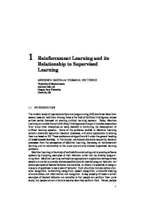
ROOT GET

pickup north

(a)

PUT

NAVIGATE TO RED

putdown

south

west

east

(b)

Figure 1. (a) Taxi domain, and (b) an action hierarchy for Taxi

5. Experiments This section presents our empirical results, which show that R- MAXQ outperforms both of its components, R- MAX and MAXQ-Q. We discuss our findings in detail, to reveal how precisely our algorithm benefits from combining modelbased learning and hierarchical decomposition.

By adapting the remainder of Kakade’s proof, we can establish that R- MAXQ will probably converge to a (recursively) near-optimal policy, although this guarantee requires exponentially more data than R- MAX in the worst case. We note that this guarantee applies to any choice of hierarchy. It remains to be seen whether it might be possible to derive tighter bounds for specific classes of action hierarchies. Furthermore, as Kakade (2003) notes in his derivation, the -approximation condition is perhaps unnecessarily stringent, since it gives the worst possible degradation in approximation quality over all possible policies.

For our experiments, we use the familiar Taxi domain (Dietterich, 2000). This domain consists of a 5 × 5 gridworld with four landmarks, labeled red, blue, green, and yellow, illustrated in Figure 1a. The agent is a taxi that must navigate this gridworld to pick up and deliver a passenger. The system has four state variables and six primitive actions. The first two state variables, x and y, give the coordinates of the taxi in the grid. The third, passenger, gives the current location of the passenger as one of the four landmarks or as taxi, if the passenger is inside the taxi. The final state variable, destination, denotes the landmark where the passenger must go. Four primitive actions, north, south, east, and west, each move the taxi in the indicated direction with probability 0.8 and in each perpendicular direction with probability 0.1. The pickup action transfers the passenger into the taxi if the taxi is at the indicated landmark. The putdown action ends an episode if the passenger is in the taxi and the taxi is at the desired destination. Each episode begins with the taxi in a random location, the passenger at a random landmark, and a destination chosen randomly from the remaining landmarks. Each action incurs a −1 penalty, except that unsuccessful pickup and putdown actions cost −10, and a successful putdown action earns a reward of 20.

In practice, implementations of R- MAX use far smaller values of m than would be required to achieve useful theoretical guarantees. In this vein, we note that running R- MAXQ will result in no more time spent in exploration than running R- MAX with the same value for m. The hierarchical decomposition only weakens the guarantees on the nearoptimality of the policy that R- MAXQ exploits. The experiments described in the next section show that a good hierarchy can even reduce the amount of time spent exploring, with no appreciable deterioration in solution quality.

The structure of the Taxi domain makes it conducive for research into hierarchical RL. The optimal policy may be described abstractly in four steps. First, navigate to the landmark where the passenger is. Second, pick up the passenger. Third, navigate to the destination landmark. Finally, put down the passenger. Navigation to each of the landmarks constitute reuseable subtasks that hierarchical algorithms can exploit. Dietterich (2000) expressed this domain knowledge in the task hierarchy shown in Figure 1b. This hierarchy defines a navigational composite action for

at each state to achieve the same error bound at the root of the hierarchy, where T is the maximum number of reachable terminal states for any composite action and h is the height of the hierarchy: the number of composite tasks on the longest path from the root of the hierarchy to a primitive action (not including the root itself).

Hierarchical Model-Based Reinforcement Learning: R- MAX + MAXQ 0

R-MAXQ R-MAX MAXQ-Q

0 Reward per episode

Cumulative reward

-10000 -20000 -30000 -40000

-20 -40 -60

-50000

R-MAXQ R-MAX MAXQ-Q

-80 -60000 0

200

400

600

800 1000 1200 1400 1600

Episodes

(a)

0

200

400

600

800

1000 1200 1400 1600

Episodes

(b)

Figure 2. (a) Cumulative and (b) asymptotic performance of R- MAXQ, R- MAX, and MAXQ-Q on the Taxi domain, averaged over 100 independent trials. R- MAXQ and MAXQ-Q utilize the hierarchy shown in Figure 1b, but they do not use any explicit state abstraction.

each of the four landmarks. These actions include the four primitive movement actions as children, and they terminate upon reaching the coordinates corresponding to the respective landmark. The GET and PUT composite actions each have all four of their navigational composite actions as children, as well as pickup or putdown, respectively. GET terminates when the passenger is in the taxi, and PUT terminates only when the episode does. The ROOT action only includes GET and PUT as children, and like PUT it defines no terminal states beyond those intrinsic to the domain. All goal reward functions give 0 reward; each action simply minimizes the costs earned before reaching their subgoals. In our experiments with R- MAX and R- MAXQ we set the threshold sample size at m = 5. Preliminary experiments showed that larger values of m did not signicantly improve the final policy, although of course they led to more time spent estimating the model. The only other parameter for these algorithms is the stopping criterion for the dynamic programming steps in Algorithms 2 and 4. In all cases, we ran value iteration until the largest change was smaller than  = 0.001. We provided R- MAXQ and the original MAXQQ algorithm with the hierarchy shown in Figure 1b as prior knowledge. For our implementation of MAXQ-Q, we used precisely the hand-tuned parameters Dietterich (2000) optimized for the initial value function, learning rates, and temperature decay (for Boltzmann exploration) for each action in the hierarchy. We conducted 100 independent trials of each condition of our experiments. 5.1. R-MAXQ versus R-MAX We begin by comparing the performance of R- MAXQ and R- MAX on the Taxi task. Our initial hypothesis was that R- MAXQ would perform no better than R- MAX in the absence of state abstraction, since the model-based ability to

plan to explore might subsume the exploratory role that options have played in many model-free RL implementations (S¸ims¸ek & Barto, 2004; Singh et al., 2005). Figure 2 reveals that in fact the two algorithms exhibit very different learning curves. In particular, although R- MAX requires many fewer episodes to converge to an optimal policy, RMAXQ earns much greater total reward. We had overlooked the fact that the hierarchy used by RMAXQ doesn’t so much guide exploration as it constrains it. In particular, note that the hierarchical agent can never attempt the putdown action except at one of the four landmark locations, since the PUT action only becomes available when the agent is already at one of these locations, and the four navigational actions keep the agent in this reduced set of states. The agent thus only attempts the putdown action in 12 incorrect states, instead of the 396 explored by R- MAX. In addition, R- MAX attempts the pickup action in 100 states in which R- MAXQ doesn’t, when the passenger is already in the car. Since the penalty for incorrect usage of these actions is -10, R- MAX loses 10(396 − 12 + 100)m = 24200 reward due to its wasted exploration, accounting for the difference between the two algorithms in Figure 2a. Furthermore, since the GET action cannot navigate to an arbitrary location, R- MAXQ can’t attempt the pickup action in a non-landmark location until some episode randomly starts the agent there. In this case the hierarchy can only postpone, not prevent, wasted exploration. This effect explains the delayed convergence relative to R- MAX: in later episodes R- MAXQ spends time on exploration that R- MAX performed more eagerly. 5.2. R-MAXQ versus MAXQ-Q Figure 2 also compares R- MAXQ with the original MAXQQ algorithm. Of course, this comparison isn’t very fair,

Hierarchical Model-Based Reinforcement Learning: R- MAX + MAXQ 0

Cumulative reward

-10000 -20000 -30000 -40000 -50000

R-MAXQ R-MAX MAXQ-Q

-60000 0

200

400

600

800 1000 1200 1400 1600

Episodes

Figure 3. Cumulative performance of R- MAXQ, R- MAX, and MAXQ-Q on the Taxi domain, using state abstraction. (The asymptotic performance is qualitatively similar to that shown in Figure 2b, although with faster convergence.)

since a primary goal of the MAXQ framework was to create opportunities for state abstraction (Dietterich, 2000), which we did not initially exploit. In fact, Dietterich identified the condition described in Section 5.1, which he called shielding, as one that permits abstraction. For a more fair comparison, we allowed our implementation of MAXQ-Q to use all the state abstractions in the Taxi domain identified by Dietterich (2000), along with his optimized parameters. We applied Dietterich’s notion of max node irrelevance to allow R- MAXQ also to enjoy an explicit form of state abstraction as prior knowledge. Each action in the hierarchy abstracts away state variables when our domain knowledge indicates that doing so would not compromise the learned model. However, whereas in MAXQ-Q an action a only reports its abstract reward function Ra to its parents, in RMAXQ it must also convey the abstract transition function P a . Thus we only allow a composite action to ignore a state variable if all of its children also ignore that state variable. In the hierarchy shown in Figure 1b, the four primitive movement actions and the four navigational actions can abstract away the passenger and destination state variables. GET and pickup ignore destination, and PUT and putdown ignore passenger. However, ROOT cannot ignore any state variables. When a child’s transition function was more abstract than a parent’s model, the parent assumed a very simple dynamic Bayes network (DBN) factorization (Boutilier et al., 1995). For example, P north sets x and y (each conditional on the previous values of both variables), but passenger and destination remain constant. Figure 3 compares the performance of the resulting algorithms. Both MAXQ-Q and R- MAXQ learn much faster with state abstraction, with the model-based nature of R- MAXQ continuing to give it an edge.

It is worthwhile to examine more closely how the hierarchy interacts with state abstraction in the Taxi domain. Consider how MAXQ-Q learns the ROOT action. The only values stored locally are the completion functions C root(·, GET) and C root(·, PUT), which have different abstract representations. The latter function is always equal to 0, since after PUT terminates there is nothing to complete, since the entire episode has terminated. Meanwhile, to evaluate C root(s, GET) the algorithm need only inspect the passenger and destination variables of s, since the values of these two variables before executing GET completely determine the remaining cost of completing ROOT after GET terminates. Hence, MAXQ-Q only learns 16 values at the ROOT node; to compute the value of a state it recursively queries Ra and adds the appropriate completion function (Dietterich, 2000). R- MAXQ doesn’t apply any explicit state abstraction to ROOT, but note that after executing either of its two child actions, the result must be one of 12 nonterminal states: with the taxi at one of four landmarks, the passenger in the taxi, and the destination at one of the other three landmarks. Hence, the planning envelope computed in Algorithm 2 will always contain some subset of these 12 states plus the current state. As with MAXQ-Q, the result distribution irrelevance of GET allows R- MAXQ to store only a small number of values locally. To compute the value of a state, R- MAXQ also queries one-step values from its children and then adds the appropriate successor state values. In this sense, these 12 states can be thought of as the completion set of ROOT. Figure 3 also shows the performance of standard R- MAX with the same DBN factorization as R- MAXQ applied to most of its actions (which are all primitive). Note that in the absence of shielding, putdown cannot safely ignore the passenger variable. The ability to abstract the primitive models does reduce the amount of exploration that R- MAX must perform, but the improvement is significantly smaller than that of the other algorithms. This result gives more support for motivating hierarchical decomposition with opportunities for state abstraction. Some preliminary further experiments support the arguments of Jong et al. (2008), who used model-free hierarchical algorithms to suggest that composite actions more reliably improve RL performance when they replace instead of augment primitive actions. We ran R- MAXQ with a hierarchy in which the root’s children included all six primitive actions as well as the four navigational composite actions, producing learning curves indistinguishable from those of standard R- MAX in Figure 2. When the root action can execute every primitive action, the planning envelope grows to include too many states. Formalizing the properties of a composite action’s completion set may help us understand

Hierarchical Model-Based Reinforcement Learning: R- MAX + MAXQ

how hierarchies can constrain planning envelopes without sacrificing learning performance.

6. Related Work Other algorithms have combined hierarchical RL with a model-based approach, but not in the standard framework of discounted rewards and stochastic dynamics. Diuk et al. (2006) developed a model-based MAXQ algorithm for deterministic domains, allowing them to quickly sample the effect of a composite action recursively: every action’s effect can be represented as a scalar reward and a single successor state. Their algorithm also uses Dietterich’s approach to state abstraction, occasionally forcing it to replan, since the effect of a child action may depend on state variables not visible to the parent, making it seem nondeterministic. In contrast, R- MAXQ does not employ explicit state abstraction, allowing it to save the value functions and policies computed during one time step for all future time steps. Our algorithm relies on the choice of hierarchy to yield small planning envelopes, automatically achieving an effective reduction in the size of the state space considered during any one time step. Seri and Tadepalli (2002) extended the MAXQ framework to average-reward reinforcement learning, resulting in an algorithm that learns a model to facilitate the computation of the bias for each state from the average reward of the current policy. However, the computation of the average reward itself relies on stochastic approximation techniques, and their algorithm does not have any formal guarantees regarding its sample complexity.

7. Conclusions The R- MAXQ algorithm combines the efficient modelbased exploration of R- MAX with the hierarchical decomposition of MAXQ. Although our algorithm does not improve upon the known formal bounds on the sample complexity of RL, it retains a finite-time convergence guarantee. An empirical evaluation demonstrates that even a relatively simple hierarchy can improve the cumulative reward earned by constraining the exploration that the agent performs, both within individual episodes of learning and throughout an agent’s experience with its environment. Even in the absence of explicit state abstraction, the structure of an action hierarchy can drastically reduce the effective state space seen by a given composite action during a single episode. This implicit concept of a reduced completion set, mirroring Dietterich’s explicitly abstracted completion function, suggests future avenues of research, both for improving the theoretical guarantees on the sample complexity of R- MAXQ and for guiding the discovery of more useful hierarchies.

Acknowledgments This material is based upon work supported by the National Science Foundation under Grant No. 0237699 and the DARPA Bootstrap Learning program.

References Barto, A. G., & Mahadevan, S. (2003). Recent advances in hierarchical reinforcement learning. Discrete-Event Systems, 13, 41–77. Special Issue on Reinforcement Learning. Boutilier, C., Dearden, R., & Goldszmidt, M. (1995). Exploiting structure in policy construction. Proceedings of the Fourteenth International Joint Conference on Artificial Intelligence (pp. 1104–1111). Brafman, R. I., & Tennenholtz, M. (2002). R-MAX – a general polynomial time algorithm for near-optimal reinforcement learning. Journal of Machine Learning Research, 3, 213–231. Dietterich, T. G. (2000). Hierarchical reinforcement learning with the MAXQ value function decomposition. Journal of Artificial Intelligence Research, 13, 227–303. Diuk, C., Strehl, A. L., & Littman, M. L. (2006). A hierarchical approach to efficient reinforcement learning in deterministic domains. Proceedings of the Fifth International Joint Conference on Autonomous Agents and Multiagent Systems. Jong, N. K., Hester, T., & Stone, P. (2008). The utility of temporal abstraction in reinforcement learning. Proceedings of the Seventh International Joint Conference on Autonomous Agents and Multiagent Systems. Kakade, S. M. (2003). On the sample complexity of reinforcement learning. Doctoral dissertation, University College London. Kearns, M., & Singh, S. (1998). Near-optimal reinforcement learning in polynomial time. Proceedings of the Fifteenth International Conference on Machine Learning (pp. 260–268). Moore, A. W., & Atkeson, C. G. (1993). Prioritized sweeping: Reinforcement learning with less data and less real time. Machine Learning, 13, 103–130. Seri, S., & Tadepalli, P. (2002). Model-based hierarchical average-reward reinforcement learning. Proceedings of the Nineteenth International Conference on Machine Learning (pp. 562–569). ¨ & Barto, A. G. (2004). Using relative novelty to S¸ims¸ek, O., identify useful temporal abstractions in reinforcement learning. Proceedings of the Twenty-First International Conference on Machine Learning (pp. 751–758). Singh, S., Barto, A. G., & Chentanez, N. (2005). Intrinsically motivated reinforcement learning. Advances in Neural Information Processing Systems 17. Sutton, R. S., & Barto, A. G. (1998). Reinforcement learning: An introduction. Cambridge, MA: MIT Press. Sutton, R. S., Precup, D., & Singh, S. (1999). Between MDPs and semi-MDPs: A framework for temporal abstraction in reinforcement learning. Artificial Intelligence, 112, 181–211.