Globalization and the Industrial Revolution Pedro Cavalcanti Ferreiray

Samuel Pessôaz

Fundação Getulio Vargas

Fundação Getulio Vargas

Marcelo Rodrigues dos Santosx Insper

Abstract This paper argues that trade specialization played an indispensable role in supporting the Industrial Revolution. We calibrate a two-good and two-sector overlapping generations model to England’s historical development and investigate how much different England’s development path would have been if it had not globalized in 1840. The open-economy model is able to closely match the data, but the closed-economy model cannot explain the fall in the value of land relative to wages observed in the 19th century. Without globalization, the transition period in the British economy would be considerably longer than that observed in the data and key variables, such as the share of labor force in agriculture, would have converged to …gures very distant from the actual ones. Key words: Industrial revolution; International trade; Malthusian trap. JEL classi…cation: F1; O1

We wish to thank seminar participants at the University of Illinois at Urbana-Champaign, the 11th Society for the Advancement of Economic Theory conference, Insper, EPGE-FGV and the 32nd Meeting of the Brazilian Econometric Society 2010, as well as two referees and the editor for their helpful comments. We are responsible for any remaining errors. The authors acknowledge the …nancial support of CNPQ/INCT and CAPES. y Graduate School of Economics, Fundação Getulio Vargas, Praia de Botafogo 190, 1125, Rio de Janeiro, RJ, 22253-900, Brazil. Email: [email protected]. z Graduate School of Economics, Fundação Getulio Vargas, Praia de Botafogo 190, 1125, Rio de Janeiro, RJ, 22253-900, Brazil. Email: [email protected]. x Insper Institute of Education and Research, Rua Quata 300, São Paulo, SP, 04546-042, Brazil. Email: [email protected].

1

1

Introduction

This article aims to show that international trade is crucial to understanding factor price dynamics and the labor share of agriculture in England during the 19th Century. This article does not provide a new theory of the Industrial Revolution, why it happened in England, or why it happened at that given period in time. This article also does not explain the boost in trade. Its main point is to show, by simulating a two-sector growth model calibrated to 18th and 19th century England, that one cannot fully explain Industrial Revolution without trade. In the model developed in this paper, the expansion of international trade takes place at about the same time that the technology in the manufacturing sector reaches a stage of development high enough to allow the economy to transit from stagnation to dynamic growth. We argue that trade specialization played an indispensable role in supporting the industrial revolution as it allowed the economy to shift resources to the production of manufactured goods without facing a shortage of food and raw material. Consequently, as opposed to onegood models (Hansen and Prescott(2002), Ngai(2004)) in which the industrial revolution is associated with a transition from the Malthusian economy to the Solow economy, in our setup the industrial revolution entails a transition towards a dynamic Heckscher-Ohlin economy. In one-good models the industrial revolution is associated with the substitution of technologies that are used to produce the same good, instead of being associated with a reallocation of resources across sectors, as appeared to be the case in England between 1750 and 1850. Hence, one-good models cannot explain some important economic changes associated with the industrial revolution - namely the massive factor reallocation from the agricultural sector to the production of manufactured goods. This movement of factors of production from a stagnant to a dynamic sector is required for the economy to take advantage of the faster productivity advance in the manufacturing sector and, as a consequence, to experience a higher increase in wages, a decrease in rents and a boost of the wage/rent ratio as observed in this period. Thus, for a model to be close to the 2

empirical facts, it is necessary to assume that at least two goods are produced: agricultural products (using land, labor and capital) and manufactured goods (using capital and labor). Moreover, in addition to two sectors, one needs trade. Closed-economy models are not able to reproduce the fall in the ratio of land values to wages that started in the middle of the 19th century, as in these models, when technical progress in manufacture accelerates, land values rise relative to wages. When we allow our arti…cial economy to trade, this ratio falls as the import of food and raw materials relaxes the land restriction and thereby the demand for land. Most explanations of the Industrial Revolution, however, tend to emphasize factors internal to the British or Western Europe economies. For instance, North and Weingast (1989) stress that England had, at least since the 17th century, a unique set of laws protecting private property and contracts, developed markets for labor and products and restrictions on royal prerogatives that brought about the right incentives to innovation and investment. Those institutions did not exist, at that time, anywhere in the world. Others, such as Landes (1969) and Mokyr (1990), place British technological advances in sectors such as textiles, steel and transportation as the key factor behind the Industrial Revolution. Mokyr (2009) emphasizes the impact of the Enlightenment and a new set of ideas concerning scienti…c research and productivity growth. Clark (2007) defends the notion that a very subtle and long process of cultural change in England, which led people to adopt habits of education, saving, hard work and the abandonment of others (in forms such as violence and impatience), is the key element in explaining growth acceleration. The so-called uni…ed growth theory (e.g., Galor and Weil(2000), Hansen and Prescott (2002), Lucas(2002), Desmet and Parente(2009)), in almost all cases, emphasizes domestic mechanisms, although these mechanisms di¤er markedly across cases. Recently, however, some authors (e.g., Clark, 2007) have suggested that the institutions conductive to growth and economic preconditions were present in many other parts of the 18th-century world. Pomeranz (2000) suggests that the densely settled core of China was

3

indistinguishable from northwestern Europe as late as 1750 in terms of "commercialization, commodi…cations of goods, land, labor, market-driven growth and adjustment by households of both fertility and labor allocation to economic trends". Allen (2009) notes that property rights were at least as secure in France and possibly in China as in England and that there is no evidence of structural breaks in interest rates after 1688; therefore, the improved investment climate was not manifest in anything …nancial, a point made also by Clark (2007). Hence, technological inventiveness and the protection of private property were necessary to the Industrial Revolution, but they were not su¢ cient. The point made by these and other authors - e.g., O´Rourke and Williamson (2005) and Findlay and O´Rourke (2007) is that if British industry had been forced to source its raw materials domestically, rather than import them, prices would have increased rapidly, as expanding levels of demand would have been restricted by domestic land endowment. Nonfarm output increased almost ninefold between 1730 and the 1860s (Clark, 2007), but the farm area per person moved from about the same to almost half that in western Europe. While the population more than tripled over the course of the Industrial Revolution, domestic agricultural output did not even double. Evidence provided by O’Rourke and Williamson (2005), however, suggests that another structural break had taken place almost at the same time that the Industrial Revolution began: the …rst great globalization shock. The authors argue that it was only with the combined in‡uence of the switch from mercantilism to free trade at the beginning of the 19th century as well as the development of new transport technologies and the sustained decline in its costs over the whole century that the great intercontinental price gaps began to disappear. As a consequence, it was only in the 19th century that large-scale international trade became possible in some basic commodities such as grain, animal products, coal and manufactured intermediates. Their estimates suggest that without the possibility of intercontinental trade, productivity growth would almost certainly have been much less than it actually was during the Industrial Revolution.

4

To summarize, it was international trade that helped …rst England and then Europe to escape from Malthusian constraints and the ghost acres of the New World (Pomeranz, 2000) had a crucial e¤ect, permitting the expansion of industry without driving up raw materials costs to prohibitive levels.1 This article models and simulates the impact of trade on the transition to modern growth in England. The calibration of the model parameters is standard and matches some targets of 18th- and 19th-century England. The model is able to replicate some main facts of the period. We compare the results with those obtained assuming a closed economy and conclude that the acceleration of productivity growth could not, on its own, explain the fall in the value of land relative to wages observed in the 19th century. Moreover, the transition in this case is much longer than that obtained when trade is possible and does not reproduce the data. Robustness exercises (e.g., advancing the date by which the economy starts to trade) did not signi…cantly change the results. Matsuyama (1992), as far as we know, is the …rst to relate industrialization and agriculture productivity to the openness of the economy. As opposed to ours, this paper is purely theoretical, with a continuous-time two-sector model of endogenous growth. Harley and Crafts (2000) and Clark, O’Rourke and Taylor (2008) use multi-sector computable general equilibrium models to study the Industrial Revolution, highlighting the importance of international trade, which is similar to the approach by Stokey (2001). The latter article has some points in common with our approach. However, among many di¤erences, it restricts its investigation to steady states, while we are interested in studying the transition between the Malthusian period and modern growth. By doing so, we are able to model and calibrate globalization and the acceleration of technical progress as happening in di¤erent moments. Moreover, by studying the transition path, we are able to show some shortcomings of closed-economy models in the uni…ed growth literature. Crafts and Harley (2004), while 1 Although Pomeranz (2000) stresses the role of the colonies in easing the land restriction Clark, O’Rourke and Taylor (2008) argue that the key factor was trade generally, not just restricted to trade with the New World colonies. For our purposes this question is not relevant and does not a¤ect our results.

5

acknowledging the importance of trade, …nd that if Britain had not increased agriculture imports after 1770, the e¤ect of on the labor share of agriculture would have been rather small. This …nding challenges our results and will be discussed later. This article is organized in four sections in addition to this introduction. In the next section, we present the model. The calibration procedure is presented in Section 3. The results are presented in Section 4, and some concluding remarks are made in Section 5

2

The Model

2.1

Technology

Technology in the agriculture sector is such that each …rm in the sector, combines labor NA , land L and capital KA to produce an agricultural good denoted by YA : Each unit in the manufacturing sector corresponds to a factory and uses only labor NM and capital KM to produce a manufactured good, denoted by YM . The technologies for the two sectors are as follows:

YA = YM =

where

A

,

M

> 1 and

M

>

A

t t0 1 A KAt NAt L

(1)

t t0 1 M KM t N M t

(2)

denote the total factor productivity growth in the

agricultural and manufacturing sectors, respectively; manufacturing technology;

2 (0; 1) and

2 (0; 1) is the capital share for the

2 (0; 1) are the capital share and the labor share

in agriculture, respectively; and t0 denotes the period in which the Industrial Revolution begins. In this economy, land is assumed to be in …xed supply and its total size is normalized to be 1. Additionally, given that the technologies above exhibit constant returns to scale,

6

it is assumed that there is one production unit in each sector. Firms behave competitively, deciding how much of each input to employ in the production process to maximize their pro…ts, taking the wage rate w; the rental rate for capital rK , and the rental rate for rent rL as given. Formally, the …rm’s problem in each sector can be written as follows:

M ax YAt

KAt ;NAt ;Lt

M ax Pt YM t

KM t ;NM t

rKt KAt

wt NAt

rKt KM t

rLt Lt ;

wt NM t ;

s:t: (1)

s:t: (2)

where Pt denotes the price of manufactured goods in terms of the agricultural good. New investment in capital in period t takes the form of currently produced units of good A that are not used for consumption. As a consequence, the supply price of capital in terms of good A is one. The aggregate capital is determined by individual savings behavior, which will be described in the next subsection. We assume that capital is depreciated at 100% each period. In the period t; given the price Pt and the aggregate stocks of capital Kt ; labor Nt and land Lt , competition in factor markets produces a wage rate wt , an interest rate rKt , a land rent rLt , and allocations of capital KAt and labor NAt , that satisfy the equations:

wt (KAt ; NAt ) =

1 t A KAt NAt

= Pt (1

rKt (KAt ; NAt ) =

1 t A KAt NAt

= Pt

rLt (KAt ; NAt ) = (1

)

) t M (Kt

t M (Kt

KAt )

KAt ) (Nt 1

(Nt

t A KAt NAt

where we use the fact that Kt = KAt + KM t and Nt = NAt + NM t : We can combine equations (3) and (4) in order to obtain:

7

NAt )

NAt )1

(3) (4) (5)

Pt (KAt ; NAt ) =

1 t A KAt NAt

(1

)

t M (Kt

KAt ) (Nt

NAt )

=

t M (Kt

1 t A KAt NAt KAt ) 1 (Nt

NAt )1 (6)

or, after some simpli…cations:

(1

KAt = ) NAt

(Kt (Nt

KAt ) NAt )

(7)

Equation (7) de…nes an e¢ cient condition for the allocation of inputs (KAt ; NAt ); given the aggregate stock of capital Kt and the labor force Nt in period t:

2.2

Preferences and demography

Households live for two periods and have preferences that depend on both goods in both periods of their lives. Young agents are endowed with one unit of labor time, which they supply inelastically. Out of their labor income, they decide how much of each good to consume and how to divide their savings between capital and land, l. Agents do not work when old and receive income from renting land and capital to …rms and from the sale of land to the young of the next generation. Hence, an agent of generation t chooses consumptions (cyAt ; cyM t ) when she is young and (coAt+t ; coM t+1 ) when she is old, investment kt+1 and lt+1 to maximize her lifetime utility given by: ln(cyAt

c) + (1

) ln cyM t + [ ln coAt+1 + (1

) ln coM t+1 ]

subject to:

: cyAt + Pt cyM t + kt+1 + qt lt+1 = wt : coAt+1 + Pt+1 coM t+1 = rKt+1 kt+1 + (rLt+1 + qt+1 )lt+1

8

where qt is the price of land in period t, and

is the intertemporal discount factor.

We assume that there is a minimum level of consumption c for good A: This assumption is in line with the literature on structural transformation (e.g., Duarte and Restuccia, 2005) and is adopted here so that the model matches the share of the labor force employed in the agricultural sector before the industrial revolution. For simplicity, we have assumed that the minimum consumption for good A is only applied in the …rst period of an individuals’life. It is straightforward to show that the consumption of each good in each period is given by:

cyAt =

1+

cyM t =

1 1+

[wt (KAt ; NAt )

c] + c and coAt+1 = rKt+1

[wt (KAt ; NAt ) Pt

c]

and coM t+1 = rKt+1

[wt (KAt ; NAt )

c]

) [wt (KAt ; NAt ) Pt+1

c]

1+

(1 1+

(8)

(9)

and the individuals’savings and the price of land satisfy:

kt+1 =

1+

[wt (KAt ; NAt )

qt+1 = rKt+1 qt

c]

qt lt+1

rLt+1

(10) (11)

Note that we are assuming that capital is obtained in this economy from the agricultural sector. In a sense we follow classical economists such as Adam Smith and Ricardo in considering that capital constitutes seeds saved from the previous period. This assumption is not entirely necessary but aims to reproduce the fact that intermediate goods and investment goods in the period were heavily composed of agricultural goods. Let Nt denote the number of households born in period t. At each period t, there are

9

Nt+1 old households and Nt young households alive. The population growth rate between periods t and t + 1 is given by gt : Because we do not model fertility choice, gt is treated as exogenous. Thus, the law of motion for the population can be written as follows:

Nt = gt Nt

2.3

(12)

1

Equilibrium

The industrial revolution is interpreted as the transition from a closed Malthus economy (where per capita income is stagnant) to a small open economy with sustained growth. However, globalization and acceleration of technical progress need not start at the same time, although in the long-run one will observe both. The transition between the two economies is assumed to begin in t0 : In this section, we present the de…nitions of the equilibrium for the economy in t < t0 and t

t0 :

The equilibrium in the (closed) Malthus economy is characterized by the stagnation of per capita income because technological progress at that stage of development is not able to overcome the pressure of population growth on the …xed land endowment. To generate a trajectory in which per capita variables remain constant over time, it is straightforward to show (Hansen and Prescott, 2002) that the population growth rate needs to be equal to 1 1

:

A

1

Thus, in the Malthus economy, we have that gt = g =

1

A

: Moreover, note that all

endogenous variables in the model at period t can be written in terms of the allocation of capital and labor between sectors; therefore, we can de…ne the equilibrium of the economy only in terms of (KAt ; NAt ). Given these considerations, an equilibrium for the economy before the Industrial Revolution can be de…ned as follows: De…nition 1 Given Kt ; Nt ; L, the price of land qt

1

and the population growth rate of

1 1

A

, an equilibrium trajectory for the Malthus economy is given by a set of input alloca-

tions (KAt ; NAt ) = (KA ; NA ) such that 8t < t0 : 10

i) The equation (7) is satis…ed; ii) The market-clearing conditions are satis…ed2 :

Kt+1 = Nt kt+1 = Nt

1+

[wt (KA ; NA )

c]

qt

(13)

where Nt lt+1 = 1:

Nt cyAt (KA ; NA ) + Nt 1 coAt (KA ; NA ) + Nt kt+1 = YAt

(14)

Nt cyM t (KA ; NA ) + Nt 1 coM t (KA ; NA ) = YM t

(15)

iii) The price of land is given by:

qt = rKt (KA ; NA )qt

1

rLt (KA ; NA )

(16)

We calculate this equilibrium as follows. First, we combine (14) with equation (7) to determine the optimal allocation of inputs across sectors, which is also consistent with the market equilibrium. Once (KAt ; NAt ) have been calculated, prices and consumption choices can also be calculated using the appropriate equations derived above. In particular, after calculating rKt and rLt using (4) and (5), we can use (16) to obtain the price of land in t and then use (13) to calculate the stock of capital in the next period. This procedure is repeated up to t = t0

1:

We assume that at t = t0 there is a positive break in technical progress3 . Global markets may or may not become integrated at t0 , it may ocurr a few periods later. At this moment, international price gaps are eliminated. As a consequence, the domestic price is now set at _

_

Pt = P , where P denotes the price of good M in terms of good A in the international market. 2

An alternative interpretation is that K represents intermediate goods rather than capital, given that investment (and, thereby, capital) goods come from the agricultural sector. Thus, when part of YA begins to be imported, part of it is eaten by the young, part of it is consumed by the old and part of it goes to the production of other agricultural goods and (mostly) industrial goods. 3 More details of this in the Calibration Section.

11

For simplicity, we assume that the domestic economy behaves as a small open economy, so _

that it takes the price P as given and any surplus (de…cit) in the market for good M (good A) is absorbed by international trade. Hence, equations (14) and (13) no longer need to be satis…ed in equilibrium. Given these considerations, an equilibrium for the open economy is de…ned as follows: _

De…nition 2 Given Kt0 ; Nt0 , L, the price of land qt0

1

and the international price P ,

an equilibrium trajectory for the dynamic economy is given by a set of input allocations (KAt ; NAt ) such that 8t

t0 :

i) (KAt ; NAt ) is a solution of the following maximization problem:

M ax :

KAt ;NAt

t A KAt NAt

+ Pt

t M t (Kt

NAt )1

KAt ) (Nt

(17)

subject to (7) ii) The population is given by (12), while the aggregate capital and the price of land are given by the following law of motions:

Kt+1 = Nt kt+1 = Nt

1+

qt = rKt (KAt ; NAt )qt

3

[wt (KAt ; NAt )

1

c]

rLt (KAt ; NAt )

qt

(18)

(19)

Calibration

The model is simulated from 1720 to 1920 and a period in the model corresponds to 20 years. The latter assumption re‡ects the fact that life expectancy in pre-industrial societies was quite small and remained so until the beginning of the 20th century. In the baseline calibration, the period of modern growth (in which technological progress accelerates) starts at t = 1800, and trade begins in 1840. Table 1 summarizes the parameter values in the 12

baseline calibration. The intertemporal discount rate, ; was set to 1. This value is consistent with a capitaloutput ratio of 2.46, which is close to the estimates of the post-1850 capital-to-output ratio of Feinstein (1978) and Maddison (1991), who report values of approximately 2.5.

Table 1: Parameter Values - Baseline Calibration Parameter

Value

Source/Target

0.27

Food consumption in England today from laborsta.ilo.org

1.00

2.5 capital-output ratio based on Maddison (1991)

0.25

Employment in agriculture in the Malthus economy

0.20

Based on Clark (1998)

0.70

Based on Clark (1998)

0.40

Based on Hansen and Prescott (2002)

Before 1800: 1.04

0.20% Average annual growth, see text

After 1800: 1.545

2.20% Average annual growth based on PWT.

c

M

A

Before 1800: 1.032 0.16% Average annual growth based on Clark (2002) After 1800: 1.18

gt

-

0.83% Average annual growth based on Clark (2002) Values are from Maddison (1991)

The consumption of subsistence is chosen so that the model matches the share of the labor force allocated in the agricultural sector before the industrial revolution. According to Allen (2000), nearly 55% of the population in pre-industrial society was employed in agriculture. Thus, by setting c = 0:25, the model generates a value of 54:43 percent for

NAt Nt

in the Malthus economy. The parameter

determines the share of income spent on the consumption of good A in

the …rst period of individuals’lives. From (8) it is easy to obtain:

13

cyAt = wt 1+

1

c wt

+

c wt

(20)

It is straightforward to show that as wt ! +1; we have intertemporal discount factor ; the parameter

cyAt wt

!

: Thus, given the

1+

is calibrated to bring

1+

close to its value

for current data. The share of food, beverages (non alcoholic and alcoholic), tobacco and clothing expenditures on total household income in the United Kingdom in 2003 was 16.1%, according to Laborsta Internet (http://laborsta.ilo.org). We set a value for

cyAt wt

= 0:27; which generates

after the transition equal to 0:135: Other values were used to check for

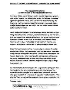
robustness and did not change the results. Of course, food consumption in the 19th century was signi…cantly higher (see Table 2.4 in Allen(2009)). However, this also happens in our case, as one can see from expression (20): for small values of w; cA is heavily in‡uenced by c; and larger than =(1 + ): Figure 1 below presents the trajectory of

cyAt wt

under the baseline

calibration. 0.4

0.35 Modern Growth 0.3

0.25

Trade

0.2

0.15

0.1

1720 1740 1760 1780 1800 1820 1840 1860 1880 1900 1920 1940

cyAt wt

Figure 1: Trajectory of

The parameter

- Baseline Calibration

associated with the technology in the manufacturing sector is set to

match physical capital’s share of income as reported by Hansen and Prescott (2002). This procedure yields a value of

= 0:4; which is a standard value for this parameter in the

growth literature. The values for the coe¢ cients on capital and labor in the agriculture sector,

and , are based on historical estimates of capital and labor shares of income by

Clark (1998). Based on this evidence, we set 14

= 0:2 and

= 0:7:

The most novel aspect of our calibration is the estimation of the structural breaks in the growth rate and in the trade regime. From the model4 one can show that the growth rate of relative prices in the Malthus economy is equal to the technological progress in the manufacturing: 1 Pt+1 = : Pt M

(21)

When modern growth starts but the economy remains closed, the growth of relative prices follows a di¤erent regime, which is a function not only of

M

but also of

A

and

population growth. In the open economy, relative prices are set in the international market, characterizing a third regime for Pt+1 =Pt : We employed the Chow test to estimate breaks in the growth rate of relative prices. The central idea of this test is to separate the initial sample in several sub-samples and to verify if the original regression delivers distinct estimators to each sub-sample. If the test identi…es di¤erent coe¢ cients between sub-samples, there exists evidence of structural break in the econometric model5 . We used the "papm" series from O´Rourke and Willianson (2005), which measures the relative prices of agricultural goods to manufacture goods in England, from 1316 to 1938 (the inverse of Pt of our model). As explained in the appendix of their article, this series was constructed from di¤erent sources. For instance, the prices of agricultural goods, pa, from 1450 to 1749, are from di¤erent volumes of the "The Agrarian History of England and Wales",6 and are “average - all agricultural products, including grains, other arable crops, livestock and animal products”. From 1805 to 1913 they were obtained from the "Abstract of British Historical Statistics" and are the total agricultural products.7 As for the prices 4

See the appendix for the derivation of this expression. More speci…cally, the model is partitioned in two or more sub-samples, each one with more observations than the number of parameters to be estimated. The Chow Structural Break Test basically compares the squared sum of residuals of the regression model with the entire sample with the squared sum of residuals resultant of the same equation for sub-samples. It uses an F-test in which the null hypothesis is no break in the period. In the present case, we test for a structural break for the trend in prices, and the model is an RA(1). 6 J. Thirsk (ed.), The Agrarian History of England and Wales, Volume IV: 1500-1640 (Cambridge: Cambridge University Press, 1967), Table XIII, p. 862. and J. Thirsk (ed.), The Agrarian History of England and Wales, Volume V: 1640-1750 (Cambridge: Cambridge University Press, 1985), Table XII, p. 856. 7 B. R. Mitchell and P. Deane, Abstract of British Historical Statistics (Cambridge: Cambridge University 5

15

of manufactured goods, in the 1450-1749 period, the series was constructed using the same source as that of pa, and the "Abstract of British Historical Statistics" was also employed for the 1796-1938 period. The series is displayed in Figure 2 below.8 Two breaks were estimated in this series, one in 1800 and the other in 1840. In the …rst case, relative prices become more positively sloped after the break, which could imply an acceleration of the growth rate of the technical progress in manufacturing. We interpret this case as the beginning of modern growth. In other words, we interpret the …rst break as a purely technological growth acceleration; as innovation in manufacturing intensi…es and resources are shifted to the sector, the prices in agriculture rise above those in manufacturing. This phenomenon is re‡ected in the steeper inclination of the relative price curve we observe after the turn of the century.

5

4.5

4

3.5

3

2.5

2 1600 1620 1640 1660 1680 1700 1720 1740 1760 1780 1800 1820 1840 1860 1880 1900 1920 1940

Figure 2: Relative Prices (PA =PM )

Subsequent to the second break, around 1840, relative prices stabilize. This re‡ects the impact of globalization: prices are now set in the international market and no longer by domestic technical progress and other local factors; otherwise, relative prices would continue to grow, as there is no evidence that innovation and technology growth reduced in this period. This estimation is close to that in O´Rourke and Willianson (2002 and 2005), albeit a bit Press, 1962). 8 We thank O’Rourke and Williamson for this and for some of the series we use in the paper.

16

later. Hence, the full integration of international markets is calibrated several decades after the acceleration of productivity growth in manufacturing, and 1840 is the estimated date of "globalization". Of course, globalization did not happen in a given year, it was a process whose rhythm was in‡uenced by a series of trade liberalization laws and measures and by innovations in transportation technology. The estimated break is capturing the year in which there is clear evidence in the data of a change of regime. Obviously, Britain had already engaged in signi…cant trade prior to 1800, but three major disruptions in trade support our calibration strategy: the continental blockage and the resulting drop in grain imports in the 1804-1814 period; the Je¤erson embargo and import prohibition from 1806 to 1809 and its lasting consequences on U.S.-Britain trade; and the Corn laws of 1815-1846, which were phased out by 1849.9 The next step is to estimate we set

M

M

for the di¤erent periods. For the Malthusian period,

= 1:04, which corresponds to a 0:2% average annual growth rate. This value is

consistent with the estimates reported by Harley and Crafts (1998). There are two alternative strategies to calibrate

M

in the modern-growth period, and they deliver di¤erent values.

One is to use estimates of technical progress in manufacturing in the 19th century reported by the economic history literature. In this case, the values range from 1%-1.4% per year in Harley (1993) and Harley and Crafts (1998) to 1.8% per year in McCloskey (1981). The problem with this approach is that it underestimates aggregate growth in later periods. The alternative is to pick

M

to match growth in the 20th century, after transition. The growth

rate of output per worker in the U.K. during the second half of the previous century was nearly 2.2%, according to the Penn-World Tables (PWT). The problem now is that this rate 9 One alternative interpretation, and one that would hurt our argument, is that the British relative price actually converged to the international relative price between 1800 and 1840. This would be consistent with the facts that trade increased in Britain before 1840 and that the relative price of agricultural products did not decline again after trade liberalization. However, even in the context of the 19th century, it seems to us that this is a rather long period for price convergence, which is generally much faster. Also against our argument, as noted before, O´Rourke and Willianson (2005) estimate that the break occurred several years earlier. To test for these hypotheses, we will run experiments opening the economy to trade before 1840.

17

overestimates technological progress in manufacturing in the 19th century. We chose the latter procedure, as it is more common one in the growth literature As for the TFP in the agricultural sector, we set and

A

A

= 1:032 for the Malthusian period

= 1:18 for the modern-growth period in the baseline calibration, corresponding to

average annual growth rates of 0.16% and 0.8%, respectively. These values are in line with the estimates reported by Clark (1998 and 2002). For robustness, we carry out a sensibility analysis in which we assume a faster growth rate for the TFP in the agricultural sector in the modern-growth period. As we abstract from endogenizing demographic decisions, the population growth is restricted to match the evolution of the English population from 1720 to 1920 as reported by Maddison (1991). We interpolate the data to obtain values for the periods for which we simulate the model.

4

Results

The economy is simulated for 11 periods initiating at t = 1720: The start of modern growth occurs at t = 1800 and globalization ocurrs at t = 1840: Figure 3 analyzes the behavior of resources allocation across sectors over time by showing the trajectories of the shares of labor force and capital stock in the agricultural sector for three di¤erent scenarios. In the …rst, the Malthus economy, per capita output and wages are constant over time and, as a consequence, there is no structural transformation as the economy evolves, as the KAt Kt

NAt Nt

and

ratios remain unchanged. In the second, "Modern Growth Only", the economy remains

closed, but there is an acceleration of technical progress in the manufacturing (from 0.2% to 2.2% per year) and agricultural (from 0.16% to 0.83% per year) sectors after t = 1800: Finally, in "Modern Growth and International Trade", there is an acceleration of technical

18

progress in 1800 as in the previous case and international trade starts at 1840: A) Labor

B) Capital 0.45 Data Data - Spline Extrapolation Malthus Modern Growth Only Modern Growth and International Trade

0.4 0.5 0.35 0.4

0.3 0.25

0.3 0.2 0.2

0.1

0 1720

0.15 0.1

Data Malthus Modern Growth Only Modern Growth and International Trade 1740

1760

1780

1800

1820

1840

0.05

1860

1880

1900

0 1720

1920

1740

1760

1780

1800

1820

1840

1860

1880

1900

1920

Figure 3: Shares of labor and capital employed in agriculture.

The model with international trade is able to replicate the structural transformation in England. As technical progress accelerates, labor and capital are shifted to manufacturing. However, when the economy is kept closed during the entire 19th century - the "Modern Growth Only" line - this movement is very slow. In fact, the simulated labor share in the agricultural sector 100 years after the increase in TFP growth rate is nearly 47% of the total. In contrast, when we allow international trade in 1840 and later - the "Modern Growth and International Trade" line - the structural transformation speeds up, and 80 years after the start of the Industrial Revolution, only 10% of the labor force still remains in the agricultural sector, which is close to the actual …gures, as one can see from the "Data" line. According to Clark(2007), nearly 21% of workers were employed in agriculture in 1860. Similarly, the trajectory of capital in the simulation with international trade follows the data better than in the closed-economy simulation. Feinstein (1988) provides …gures for the real capital stock and its allocation across sectors for 1780-1850. The data are also presented in Panel B) of Figure 3 with its extrapolation for 1860 and 1880. As shown, the closed-economy simulation can not account for the large fall in the capital share employed in agriculture during the 19th century. As a matter of fact, while the spline extrapolation for 1880 suggests a decrease in

KAt Kt

of 77% between 1780-1880, the model simulations with 19

and without international trade predict a fall in the same period of nearly 23% and 90%, respectively. Note that although we assumed acceleration of technical progress in agriculture after t = 1800; the escape from the Malthus economy in the closed-economy model is much longer than that observed in the data. This is so because in the economy with two goods without international trade, the balanced growth trajectory requires that a massive amount of resources remains allocated in the agricultural sector over time. Otherwise there would be a disequilibrium in that sector as the production of good A decreases with the reallocation of inputs towards the production of good M: In contrast, the opening of the economy to the global market allows factor reallocation to take place much faster, as any market disequilibrium can be absorbed by international trade. As a consequence, a relatively faster structural transformation can only be explained, in a speci…c factors world in which two commodities are produced, by a globalization shock which entails a great increase in the intercontinental trade. Figure 4 below presents the behavior of the land value-wages ratio. By construction it is constant in the Malthus period. According to the data (O´Rourke and Willianson (2002)), it increased very slowly in the 18th century, less than 9% during the whole period10 . However, in the …rst four decades of the 19th century, the land value-wages ratio increased by almost 40%, more than six times faster than in the previous century. Only after 1840 did it start to fall. As technical progress speeds up in manufacturing and resources are transferred to this sector, the prices of agriculture goods and land increase. Hence, income distributions change, hurting workers whose consumption basket at that time consisted mostly of food and beverages. The model is able to reproduce this fact in the …rst two periods after the start of the Industrial Revolution, when the economy is still closed. Feinstein (1998) had already noted that workers did not bene…t from growth in the beginning of the Industrial Revolution, but 10

Note, however, that the land value-wages ratio increased substantialy in the 16th and 17th centuries.

20

a large part of the literature ignores this fact. In these articles, the start of the transition to modern growth and the fall of the land value-wages ratio are simultaneous. A) Land Value-Wages ratio

B) Output Per Capita

140

700

120

600

100

500

80

400

60

300

40

Data Malthus Modern Growth Only Modern Growth and International Trade

200 Data Malthus

20

100

Modern Growth Only Modern Growth and International Trade

0 1720

1740

1760

1780

1800

1820

1840

1860

1880

0 1720

1900

1740

1760

1780

1800

1820

1840

1860

1880

1900

Figure 4: Land value-wages ratio and output per capita are both normalized to 100 in 1780.

It is only after the start of trade specialization that wages increase relative to land value. In this case, the model shows that global market integration cuts the link between factor prices and the domestic land-labor ratio, allowing the economy to overcome the pressure of population growth - and the transfers of factors to manufacturing - on the …xed land endowment. Moreover, as shown by the "Modern Growth Only" simulation in Figure 4, had the economy remained closed, the land value-wages ratio would have continued to expand, which is exactly opposite of the observed trend: from 1840 to 1900, it fell by 35%. This is another piece of evidence that trade specialization is key to explaining stylized facts of the transition to modern growth in multi-sector economies. Panel B in Figure 4 and the third line in Table 2 show the results of output per capita simulations. In the case in which we keep the economy closed ("Modern Growth Only"), the model misses the output trend by a signi…cant margin, and after 100 years - i.e., t = 1900 – the output per capita is less than 50% of the observed …gures. However, when we allow international trade to take place in 1840 and beyond, the model predicts an output per

21

capital in 1900 that is much closer to the actual …gures. Table 2: Simulations Result - Baseline Calibration 1840

1860

1880

Trade No Trade Trade No Trade Trade No Trade Agricultural Employment (%)

21.92

50.57

8.90

49.58

3.60

48.65

Land Value-Wages Ratio

30.71

115.0

12.75

118.9

3.84

122.2

Output per Capita

197.9

158.1

287.3

185.3

413.5

216.7

Capital Stock

377.6

241.0

735.1

345.1

1339

489.7

Note: All series, with the exception of agricultural employment, are normalized to 100 in 1780.

As opposed to the results above, and those in O´Rourke and Williansons (2005), Crafts and Harley (2004) …nd that trade had a rather small e¤ect: if Britain had not increased agricultural imports after 1770, the share of agricultural employment would have been 26 percent instead of 22 percent in 1841. In our case, agricultural employment without trade would have been twice as large as it would have been with trade in 1840. These authors use a CGE model that has many sectors, and the saving decision is exogenous. It may be the case (equations are not presented in the article) that the service sector, which is very large in 1841 in their model, does not use agriculture goods as inputs; therefore, trade restrictions do not hurt the service sector, which generates a smaller impact on the economy. In our case, in contrast, we only have two sectors, agriculture and non-agriculture ("manufacturing"), and the latter uses agricultural goods as inputs, which may lead to the stronger impact of international trade. Note, however, that Crafts and Harley (2004) do not match the land value-wages ratio that is much higher in their "no trade" simulation than in the data. Moreover, as they simulate only two steady states, 1770 and 1841 (while we simulate the transition up to 1920), one could suspect that if they had run their model up to, say, 1880, their simulation still would have found higher prices of agricultural goods and a higher land rent-wages ratio, 22

further worsening their match. Hence, in this key dimension, trade is very important in their model, as is the case in our model.

4.1 4.1.1

Sensitivity analysis Faster technical progress in the agricultural sector

In the benchmark calibration, technical progress in the agricultural sector rises from 0.16% annually during the Malthusian period to 0.80% after 1800. One could argue that our calibration biases the exercise against the modern growth model and in favor of the trade model because the productivity increase in agriculture is still modest when compared to the data. However, without international trade, even a large acceleration of productivity growth in the agricultural sector cannot account for the fall in the value of the land value-wages ratio; therefore, it cannot explain the reduction of income inequality associated with the Industrial Revolution. In addition, it still misses the path of employment share in agriculture by a signi…cant margin. Figure 5 presents the trajectories of the share of employment in agriculture (Panel A) and the land value-wages ratio (Panel B) for di¤erent rates of technological progress in agriculture after 1780. The horizontal line corresponds to the Malthus Economy, in which the agricultural TFP growth rate is 0:16% per year. In addition to the benchmark case where the TFP in agriculture grew at 0:83% per year after 1800, we show the results of simulating the model using a considerably higher rate, 2:2%, which is well above estimations in the literature.

23

A) Employment in Agriculture (% of total)

B) Land Value-Wages Ratio

0.6

140

0.55 120

0.5 0.45

100

0.4 0.35

80

0.3 60

0.25 0.2 0.15 0.1 1720

Data Malthus Economy Modern Growth Only: 0.80% Modern Growth Only: 2.20% 1740

1760

1780

1800

Data Malthus Economy Modern Growth Only: 0.80% Modern Growth Only: 2.20%

40

1820

1840

1860

1880

20 1720

1900

1740

1760

1780

1800

1820

1840

1860

1880

1900

Figure 4: Share of employment in agriculture and land value-wages ratio for di¤erent TFP growth rates in agriculture.

As one can seem from the …gures, without international trade, even an unrealistically high acceleration of productivity growth in agriculture cannot account for the fall in the employment share in agriculture or the fall of the land value-wages ratio. The reason for this fact is that in the balanced growth path of the closed economy, factor prices and land and labor endowments are associated over time. As a consequence, the growth of per capita output and wages must be governed by technological progress in the agricultural sector. However, given that this sector is much less capital intensive than the manufacturing sector, economic growth under that trajectory is lower, and as a result, it cannot surpass population growth, which causes the land value-wages ratio to increase during the transition. At the limit, the per capita economic growth rate without commerce 1

converges to

1

A

. Moreover, given the large share of the labor force still allocated to

agriculture after the convergence, the value of land relative to wages also remains high in the new steady state. In contrast, even when the TFP in agriculture grows 2:2% per year, the match of the model with trade remains very good, replicating almost exactly the labor share of agriculture in 1860 and following closely the fall of the land value-wages ratio after 1840. Whereas in 24

the data, the share of workers in agriculture was 10% in 1880, the simulation …gure for the open-economy model is 11.6%, as one can see from Table 3. Without trade, employment in agriculture is 45% of total, which is better than the …gure found within the baseline calibration but still very far from the actual value. Table 3: Simulation Results when TFP in Agriculture Grows 2:2% per year 1840

1860

1880

Trade No Trade Trade No Trade Trade No Trade Agricultural Employment (%)

38.74

46.58

22.84

45.55

11.60

44.81

Land Value-Wages Ratio

46.51

130.5

23.49

134.6

10.97

137.1

Output per Capita

413.9

387.9

746.7

614.5

1380

969.2

Capital Stock

633.3

491.7

1548

966.3

3621

1847

Note: All series, with the exception of agricultural employment, are normalized to 100 in 1780.

4.1.2

Opening the economy earlier

Mokyr (2009) argues that trade liberalization had already started in the 1820s, which is supported by the empirical tests from O’Rourke and Williamson (2002) in which the structural break is dated in 1828 and not 1840. In the …gures below, we present the results of a simulation in which the economy opens up to international trade in 1820 and not 1840. The match of our model does not change considerably when considering the share of workers in agriculture but worsens somewhat with respect to the land value-wages ratio. This is so because this ratio still increases after 1800 in the data, but in the simulation, after a small increase in this year, it falls quickly. As argued before, an open-economy model cannot reproduce the increase in rents and land relative to wages in the beginning of the 19th century, and opening the economy to trade earlier worsens the match in this dimension.

25

A) Labor

B) Land Value-Wages ratio 140

120

0.5

100 0.4 80 0.3 60 0.2 40 Data

0.1

Data

Malthus

20

Modern Grow th Only Modern Grow th and International Trade

0 1720

1740

1760

1780

1800

1820

1840

Malthus Modern Grow th Only Modern Grow th and International Trade

1860

1880

1900

0 1720

1920

1740

1760

1780

1800

1820

1840

1860

1880

1900

Figure 5: Economy’s dynamics when international trade starts in 1820.

We conducted other robustness exercises, and the overall results did not change. In one case, we allowed the acceleration of technological progress to start in 1780 rather than in 1800 as in the baseline calibration and the …gures obtained are similar to those presented above. In another experiment, instead of using data from Maddison (1991), we employed a population growth function restricted to roughly match the English population growth rates from 1750 to 1950. According to the evidence reported by Lucas (2002), the population growth rate seems to increase linearly in consumption until living standards become twice as large as in the Malthusian equilibrium. Afterwards, the population growth rate decreases linearly in consumption until living standards become 18 times the level observed in the Malthusian steady state. For simplicity, it is assumed that the population growth rate remains constant after that point. We use the consumption of good A of the young as a measure of living standards in the model. Once again, the main results did not change signi…cantly.

5

Conclusion

Modern growth, understood as the escape from the Malthusian trap, started before the …rst wave of globalization. Trade liberalization and innovations in transportation technology in 26

the mid-19th century allowed for the integration of markets and strong growth in international exchange. Technical progress in manufacturing accelerated decades beforehand; according to our estimates, it accelerated approximately forty years earlier, although many studies set it at di¤erent dates (in general, in the late 18th century). There are several ways to escape the Malthusian trap: an increase in agricultural productivity (Allen, 2009) or demographic change related to education (Doepke and Zilibotti, 2005, Boucekkine, de la Croix and Licandro, 2003). However, in this article, we showed that any model or theory would have a di¢ cult time in completely explaining the Industrial Revolution without international trade. We used a very simple recursive model and assumed technical progress and globalization to be exogenous. However, this simple framework is su¢ cient to make the point that without trade, England would not have been able to shift resources to the production of manufacturing goods at the rate observed in the data. This point had been made before, but we measured and showed that the transition period in the closed economy model would be considerably longer than that observed in the data and that key variables such as the share of the labor force in agriculture would converge to …gures very distant from the actual ones. Moreover, one-sector closed-economy models are not able to reproduce the fall in the ratio of land values to wage that started in the middle of the 19th century. It was only during the two periods in which our model economy remained closed but technical progress in manufacture accelerated that land values increased relative to wages. When we allow our arti…cial economy to trade, this ratio falls, as the import of food and raw materials relaxes the land restriction and the demand for land.

References [1] Allen, R. (2000) "Economic Structure and Agricultural Productivity in Europe, 13001800," European Review of Economic History, Vol. 3, pp. 1-25.

27

[2] Allen, R. (2009) "The British Industrial Revolution in Global Perspective", Cambridge. [3] Boucekkine, R., de la Croix, D., Licandro, O., (2003) "Early Mortality Declines at the Dawn of Modern Growth. Scandinavian Journal of Economics 105 (3), 401–418. [4] Clark, G. (1998) "Microbes and markets: Was the black death an economic revolution." Unpublished manuscript, University of California, Davis, 1998. [5] Clark, G. (2002) "The Agricultural Revolution? England,1500-1912." Working Paper, University of California, Davis [6] Clark, G. (2007) A Farewell to Alms: A Brief Economic History of the World. Princeton,New Jersey: Princeton University Press. [7] Clark, G.; O’Rourke, K. and A. Taylor (2009) “Made in America? The New World, The Old, and the Industrial Revolution”, NBER Working Paper 14077. [8] Crafts, N.F.R. and C.K. Harley (2004). "Precocious British Industrialization: A General-Equilibrium Perspective." in L.P. de la Escosura (ed.). Exceptionalism and Industrialization: Britain and its European Rivals, 1688-1815. Cambridge: Cambridge University Press, pp 86-107. [9] Desmet, K. and S. Parente (2009) "The Evolution of Markets and the Revolution of Industry: a Quantitative Model of England´s Development: 1300-2000," manuscript. [10] Doepke, M. and F. Zilibotti. (2005). “The Macroeconomics of Child Labor Regulation”, American Economic Review, 95, pp. 1492-1524. [11] Duarte, M. and Restuccia, D., (2005) "The Role of the Structural Transformation in Aggregate Productivity", University of Toronto. [12] Feinstein, C., (1998)

“Pessimism Perpetuated: Real Wages and the Standard of Liv-

ing in Britain During and After the Industrial Revolution.” Journal of Economic History,September , 58(3), pp. 625-658. 28

[13] Findlay, R. and K.H. O’Rourke, (2007) "Power and Plenty: Trade, War, and the World Economy in the Second Millennium," Princeton, NJ: Princeton University Press. [14] Galor, O. and D. Weil, (2000), “Population, Technology, and Growth: From Malthusian Stagnation to the Demographic Transition and Beyond,” American Economic Review, 90(4), pp. 806-828. [15] Hansen, G. and E.C. Prescott, (2002) “From Malthus to Solow,”American Economic Review, , 92(4), pp. 1205-1217. [16] Harley, C. K. (1993) “Reassessing the Industrial Revolution: A Macro View,” in J. Mokyr (ed.), "The British Industrial Revolution: An Economic Perspective," Westview Press. [17] Harley, C.K. and Crafts, N.F.R., (1998). "Productivity of Growth During the First Industrial Revolution: Inferences from the Pattern of British External Trade," Economic History Working Papers 22396, London School of Economics and Political Science, Department of Economic History. [18] Harley, C.K. and Crafts, N.F.R., (2000) "Simulating the Two Views of the British Industrial Revolution. Journal of Economic History," 60: 819-841. [19] Landes, D (1969) "The Unbound Prometheus," Cambridge. [20] Lucas, R. (2002), “The Industrial Revolution: Past and Future.” in Lectures on Economic Growth, Cambridge: Harvard University Press, pp. 109-188. [21] Maddison, A. (1991) "Dynamic Forces in Capitalist Development: a Long-run Comparative View," Oxford, Oxford University Press. [22] Matsuyama. K. (1992). "Agricultural Productivity, Comparative Advantage, and Economic Growth." Journal of Economic Theory, 58, pp. 317-34.

29

[23] McCloskey, D. (1981) "The Industrial Revolution: a Survey", in R.C. Flound and D. McCloskey (eds.), The Economic History of Britain Since 1700, Vol.1", Cambridge, Cambridge University Press. [24] Mokyr, J. (1990), "The Lever of Riches: Technological Creativity and Economic Progress," New York and London: Oxford University Press. [25] Mokyr, J (1993) "Editors Introduction: The New Economic History and the Industrial Revolution" in Joel Mokyr (ed.), "The British Industrial Revolution: An Economic Perspective,’Westview Press. 1993 [26] Mokyr, J. (2009) "The Enlightened Economy: An Economic History of Britain 17001850," Penguin Press. [27] Ngai, R. (2004) “Barriers and the Transition to Modern Growth,”Journal of Monetary Economics, October, 51(7), pp.1353-1383. [28] North, D. C. and B. Weingast (1989) “Constitution and Commitment: The Evolution of Institutional Governing Public Choice in Seventeenth-Century England”, The Journal of Economic History, 49/4: 803-832. [29] O’Rourke, K. and J. Williamson (2002) “When Did Globalization Begin?” European Review of Economic History, 6 (April):23-50. [30] O´Rourke , K. and J. Willianson (2005) "From Malthus to Ohlin: Trade, Industrialization and Distribution Since 1500," Journal of Economic Growth, Springer, vol. 10(1), pages 5-34, 01. [31] Pomeranz, K. (2000) "The Great Divergence: China, Europe, and the Making of the Modern World Economy." Princeton, NJ: Princeton University Press. [32] Stokey, N. L. (2001) “A Quantitative Model of the British Industrial Revolution,1780– 1850.”Carnegie-Rochester Conference Series on Public Policy, 55: 55–109. 30

Appendix Relative price is given by:

Pt =

1 t t0 A KAt NAt

(1

)

t t0 M

(Kt

KAt ) (Nt

(22)

NAt )

so that its growth rate is: Pt+1 = Pt

1 t+1 t0 KAt+1 NAt+1 A 1 t t0 A KAt NAt

(1 (1

t t0 M

)

t+1 t0 M

)

(Kt

KAt ) (Nt

(Kt+1

NAt )

KAt+1 ) (Nt+1

NAt+1 )

which simpli…es to Pt+1 = Pt

KAt+1 KAt

A M

1

NAt+1 NAt

Kt+1 KAt+1 Kt KAt

:

Nt+1 NAt+1 Nt NAt

Using the fact that the capital-labor ratio is constant, capital and labor grows at the same ratio g Pt+1 = Pt It is easy to show that g =

1 1 ( + )

A

A

+

g

M

1

=

g

A

g

+

1

M

; so that

Pt+1 = Pt

A M

1

=

1

A

(23)

:

M

When modern growth starts, but the economy remains closed, the growth of relative prices follows a di¤erent regime, which is a function not only of

M

but also of

A

and

population growth. More precisely, it is possible to show that, after lengthy calculations, in the long-run Pt+1 1 = Pt M where

N

A 1 ( + ) N

! 11

is the population growth rate, assumed to be exogenous.

31