Geometric Camera Calibration Juho Kannala, Janne Heikkil¨a and Sami S. Brandt University of Oulu, Finland January 7, 2008

Abstract Geometric camera calibration is a prerequisite for making accurate geometric measurements from image data and it is hence a fundamental task in computer vision. This article gives a discussion about the camera models and calibration methods used in the field. The emphasis is on conventional calibration methods where the parameters of the camera model are determined by using images of a calibration object whose geometric properties are known. The presented techniques are illustrated with real calibration examples where several different kinds of cameras are calibrated using a planar calibration object.

1

Introduction

Geometric camera calibration is the process of determining geometric properties of a camera. Here the camera is considered as a ray-based sensing device and the camera geometry defines how the observed rays of light are mapped onto the image. The purpose of calibration is to discover the mapping between the rays and image points. Hence, a calibrated camera can be used as a direction sensor where both the forward-projection and back-projection are known, i.e., one may compute the image point corresponding to a given projection ray and vice versa. The geometric calibration of a camera is usually performed by imaging a calibration object whose geometric properties are known. The calibration object often consists of one to three planes which contain visible control points in known positions. The calibration is achieved by fitting a camera model to the observations which are the measured positions of the control points in the calibration images. The camera model contains two kinds of parameters: the external parameters relate the camera orientation and position to the object coordinate frame and the internal parameters determine the projection from the camera coordinate frame onto image coordinates. Typically, both the external and internal camera parameters are estimated in the calibration process which usually involves non-linear optimization and minimizes a suitable cost function over the camera parameters. The sum of squared distances between the measured and modeled control point projections is frequently used as the cost function since it gives the maximum-likelihood parameter estimates assuming isotropic and independent normally distributed measurement errors. 1

Calibration by non-linear optimization requires a good initial guess for the camera parameters. Hence, various methods have been proposed for the direct estimation of the parameters. Most of these methods deal with conventional perspective cameras but recently there has also been effort in developing models and calibration methods for more general cameras. In fact, the choice of a suitable camera model is an important issue in camera calibration. For example, the pinhole camera model, which is based on the ideal perspective projection model and often used for conventional cameras, is not a suitable model for omnidirectional cameras which have a very large field of view. Hence, there has been a recent trend towards generic calibration techniques which would allow the calibration of various types of cameras. In this article, we will provide an overview into geometric camera calibration and its present state-of-the-art. However, since the literature for camera calibration is vast and ever-evolving it is not possible to cover all the aspects in detail. Nevertheless, we hope that this article serves as an introduction to the literature where more details can be found. The article is hence structured as follows. First, in Section 2, we describe some historical background for camera calibration. Thereafter we review different camera models with an emphasis on central cameras. After describing camera models we discuss methods for camera calibration. The focus is on our previous works [1, 2]. Finally, in Section 5, we present some calibration examples with real cameras. The article is concluded in Section 6.

2

Background

Geometric camera calibration is a prerequisite for image-based metric 3D measurements and it has a long history in photogrammetry and computer vision. One of the first references is by Conrady [3] who derived an analytical expression for the geometric distortion in a decentered lens system. Conrady’s model for decentering distortion was used by Brown [4] who proposed a plumb line method for calibrating radial and decentering distortion. Later on the approach used by Brown was commonly adopted in photogrammetric camera calibration [5]. In photogrammetry, the emphasis has traditionally been in the rigorous geometric modeling of the camera and optics. On the other hand, in computer vision it is considered important that the calibration procedure is automatic and fast. For example, the well-known calibration method developed by Tsai [6] was designed to be an automatic and efficient calibration technique for machine vision metrology. This method uses a simpler camera model than [4] and avoids the full-scale non-linear search by using simplifying approximations. However, due to the increased processing power of personal computers the non-linear optimization is not as time-consuming now as it was before. Hence, when the calibration accuracy is important the camera parameters are usually refined by a full-scale non-linear optimization. Besides increasing the theoretical understanding, the advances in geometric computer vision have also affected the practice of image-based 3D reconstruction during the last two decades [7,8]. For example, while the traditional photogrammetric approach assumes a pre-calibrated camera, an alternative approach is to compute a projective reconstruction with an uncalibrated perspective camera. The projective reconstruction is defined up to a 3D projective transformation

2

and it can be upgraded to a metric reconstruction by self-calibration [8]. In self-calibration the camera parameters are determined without a calibration object; feature correspondences over multiple images are used instead. However, the conventional calibration is typically more accurate and stable than self-calibration. In fact, self-calibration methods are beyond the scope of this article.

3

Camera models

In this section we describe several camera models which have appeared in the literature. We concentrate on central cameras, i.e., cameras with a single effective viewpoint. Single viewpoint means that all the rays of light arriving onto the image travel through a single point in space.

3.1

Perspective cameras

The pinhole camera model is the most common camera model and it is a fair approximation for most conventional cameras which obey the perspective model. Typically these conventional cameras have a small field of view (< 60 ◦ ). The pinhole camera model is widely used and simple; essentially it is just a perspective projection followed by an affine transformation in the image plane. The pinhole camera geometry is illustrated in Fig. 1. In a pinhole camera the projection rays meet at a single point which is the camera center C and its distance from the image plane is the focal length f . By similar triangles, it may be seen in Fig. 1 that the point (Xc , Yc , Zc )> in the camera coordinate frame is projected to the point (f Xc /Zc , f Yc /Zc )> in the image coordinate frame. In terms of homogeneous coordinates this perspective projection can be represented by a 3 × 4 projection matrix,    X    f 0 0 0  c x  y  '  0 f 0 0   Yc   Zc  0 0 1 0 1 1 where ' denotes equality up to scale. However, instead of the image coordinates (x, y)> , the pixel coordinates (u, v)> are usually used and they are obtained by the affine transformation        u0 u mu −mu cot α x + , (1) = mv y v0 v 0 sin α where (u0 , v0 )> is the principal point, α is the angle between u and v axis, and mu and mv give the number of pixels per unit distance in u and v directions, respectively. The angle α is π2 in the conventional case of orthogonal pixel coordinate axes. In practice, the 3D point is expressed in some world coordinate system that is different from the camera coordinate system. The motion between these coordinate systems is given by a rotation R and translation t. Hence, in homogeneous

3

PSfrag replacements

Z O

u

Y

α v

X

X

R, t

m p

C

Xc

Zc

x

f

y

principal axis

image plane Yc

Figure 1: Pinhole camera model. Here C is the camera center and the origin of the camera coordinate frame. The principal point p is the origin of the normalized image coordinate system (x, y). The pixel image coordinate system is (u, v). coordinates, the mapping of the 3D point X to its image m is     mu −mu cot α u0 f 0 0 0  R t mv    v 0 f 0 0 m' 0 X 0 sin α 0 1 0 0 1 0 0 1 0    mu f mu sf mu f −mu f cot α u0   mv  R t X= 0 mu γf f v = 0 0 sin α 0 0 0 0 1

given by

 u0  v0  R 1

 t X (2)

v where we have introduced the parameters γ = mumsin α and s = − cot α in order to simplify the notation. Since a change in the focal length and a change in the pixel units are indistinguishable above we may set mu = 1 and write the projection equation in the form   m ' K R t X, (3)

where the upper triangular matrix 

f K=0 0

sf γf 0

 u0 v0  1

(4)

is the camera calibration matrix and contains the five internal parameters of a pinhole camera. It follows from Eq. (3) that a general pinhole camera may be represented by a homogeneous 3 × 4 matrix   P=K R t (5) 4

which is called the camera projection matrix. If the left hand submatrix KR is non-singular, as it is for perspective cameras, the camera P is called a finite projective camera. A camera represented by an arbitrary homogeneous 3 × 4 matrix of rank 3 is called a general projective camera. This class covers the affine cameras which have a projection matrix whose last row is (0, 0, 0, 1) up to scale. A common example of an affine camera is the orthographic camera where the scene points are orthogonally projected onto the image plane. 3.1.1

Lens distortion

The pinhole camera is an idealized mathematical model for real cameras which may often deviate from the ideal perspective imaging model. Hence, the basic pinhole model is often accompanied with lens distortion models for more accurate calibration of real lens systems. The most important type of geometric distortion is the radial distortion which causes an inward or outward displacement of a given image point from its ideal location. Decentering of lens elements causes additional distortion which also has tangential components. A commonly used model for lens distortion accounts for radial and decentering distortion [4,5]. According to this model the corrected image coordinates x0 , y 0 are obtained by x0 = x + x ¯ (κ1 r2 + κ2 r4 + κ3 r6 + . . .)

+ ρ1 (r2 + 2¯ x2 ) + 2ρ2 x ¯y¯ 1 + ρ3 r2 + . . .

y 0 = y + y¯ (κ1 r2 + κ2 r4 + κ3 r6 + . . .)

+ 2ρ1 x ¯y¯ + ρ2 (r2 + 2¯ y 2 ) 1 + ρ3 r 2 + . . . ,

(6)

where x and y are the measured coordinates, and

x ¯ = x − xp y¯ = y − yp q r = (x − xp )2 + (y − yp )2 . Here the center of distortion (xp , yp ) is a free parameter in addition to the radial distortion coefficients κi and decentering distortion coefficients ρi . In the traditional photogrammetric approach the values for the distortion parameters are computed by least-squares adjustment by requiring that images of straight lines are straight after the correction [4]. However, the problem with this approach is that not only the distortion coefficients but also the other camera parameters are initially unknown. For example, the formulation above requires that the scales in both coordinate directions are equal which is not the case with pixel coordinates unless the pixels are square. In [1] the distortion model of Eq. (6) was adapted and combined with the pinhole model in order to make a complete and accurate model for real cameras. This camera model has the form m = P(X) = PX + C(PX),

(7)

where P denotes the non-linear camera projection and P is the camera projection matrix of a pinhole camera. The non-linear part C is the distortion model 5

PSfrag replacements

PSfrag replacements

orthographic

F

PSfrag replacements

orthographic

F

perspective

hyperbolic mirror P

F

elliptical mirror

P

F0

parabolic mirror P

F0

F0 perspective

parabolic elliptical

p

camera parabolic hyperbolic

orthographic camera

perspective camera p

Z

Z

hyperbolic elliptical

p Z

Figure 2: Central catadioptric camera with a hyperbolic, elliptical and parabolic mirror. The Z-axis is the optical axis of the camera and the axis of revolution for the mirror surface. The scene point P is imaged at p. In each case the viewpoint of the catadioptric system is the focal point of the mirror denoted by F . In the case of hyperbolic and elliptical mirrors the effective pinhole of the perspective camera must be placed at the other focal point which is here denoted by F 0 . derived from Eq. (6). In [1], two parameters were used for both the radial and decentering distortion, i.e. the parameters κ1 , κ2 and ρ1 , ρ2 , and it was assumed that the center of distortion coincides with the principal point of the pinhole camera.

3.2

Central omnidirectional cameras

Although the pinhole model accompanied with lens distortion models is a fair approximation for most conventional cameras, it is not a suitable model for omnidirectional cameras whose field of view is over 180◦ . This is due to the fact that, when the angle between the incoming light ray and the optical axis of the camera approaches 90◦ , the perspective projection maps the ray infinitely far in the image and it is not possible to remove this singularity with the distortion model described above. Hence, more flexible models are needed and below we discuss different models for central omnidirectional cameras. 3.2.1

Catadioptric cameras

In a catadioptric omnidirectional camera the wide field of view is achieved by placing a mirror in front of the camera lens. In a central catadioptric camera the shape and configuration of the mirror are such that the complete catadioptric system has a single effective viewpoint. It has been shown that the mirror surfaces which produce a single viewpoint are surfaces of revolution whose twodimensional profile is a conic section [9]. Practically useful mirror surfaces used in real central catadioptric cameras are planar, hyperbolic, elliptical and parabolic. However, a planar mirror does not change the field of view of the camera [9]. The central catadioptric configurations with hyperbolic, elliptical and parabolic mirrors are illustrated in Fig. 2. In order to satisfy the single viewpoint constraint the parabolic mirror is combined with an orthographic camera while 6

the other mirrors are combined with a perspective camera. In each case the effective viewpoint of the catadioptric system is the focal point of the mirror denoted by F in Fig. 2. Single-viewpoint catadioptric image formation is well studied [9, 10] and it has been shown that a central catadioptric projection, including the cases shown in Fig. 2, is equivalent to a two-step mapping via the unit sphere [10, 11]. As described in [11, 12], the unifying model for central catadioptric cameras may be represented by a composed function H ◦ F so that m = (H ◦ F)(Φ),

(8)

where Φ = (θ, ϕ)> defines the direction of the incoming light ray which is mapped to the image point m = (u, v, 1)> . Here F first projects the object point onto a virtual image plane and then the planar projective transformation H maps the virtual image point to the observed image point m. The two-step mapping F is illustrated in Fig. 3(a), where the object point X is first projected
> to q = cos ϕ sin θ, sin ϕ sin θ, cos θ on the unit sphere, whose center O is the effective viewpoint of the camera. Thereafter the point q is perspectively projected to x from another point Q so that the line determined by O and Q is perpendicular to the image plane. The distance l = |OQ| is a parameter of the catadioptric camera. Mathematically the function F has the form   cos ϕ x = F(Φ) = r(θ) , (9) sin ϕ where the function r is the radial projection which does not depend on ϕ due to radial symmetry. The precise form of r as a function of θ is determined by the parameter l, i.e., (l + 1) sin θ . (10) r= l + cos θ This follows from the fact that the corresponding sides of similar triangles must l+1 have the same ratio, thus sinr θ = l+cos θ , as Fig. 3(a) illustrates. In a central catadioptric system with a hyperbolic or elliptical mirror the camera axis does not have to be aligned with the mirror symmetry axis. The camera can be rotated with respect to the mirror as long as the camera center is at the focal point of the mirror. Hence, in the general case, the mapping H from the virtual image plane to the real image plane is a planar projective transformation [12]. However, often the axes of the camera and mirror are close to collinear so that the mapping H can be approximated with an affine transformation A [11]. That is,   x m = A(x) = K , (11) 1 where the upper triangular matrix K is defined in Eq. (4) and contains five parameters. (Here the affine transformation A has only five degrees of freedom since we may always fix the camera coordinate frame so that the x-axis is parallel to the u-axis.)

7

PSfrag replacements

PSfrag replacements Q O x X q l sin θ cos θ (12) (10)

(12) (10)

l X

O

(i) (ii) (iii) (iv) X (v)

θ

π 2

q x

r

X Z

Q

(i) (ii)

2

(iii) (iv)

cos θ

1

(v)

sin θ

r

0

Z

0

1

π 2

θ

(b)

(a)

Figure 3: (a) A generic model for a central catadioptric camera [11]. The Zaxis is the optical axis and the plane Z = 1 is the virtual image plane. The object point X is first projected to q on the unit sphere and thereafter q is perspectively projected to x from Q. (b) The projections of Eqs. (12)-(16). 3.2.2

Fish-eye lenses

Fish-eye cameras achieve a large field of view by using only lenses while the catadioptric cameras use both mirrors and lenses. Fish-eye lenses are designed to cover the whole hemispherical field in front of the camera and the angle of view is very large, possibly over 180◦ . Since it is impossible to project the hemispherical field of view on a finite image plane by a perspective projection the fish-eye lenses are designed to obey some other projection model [13]. The perspective projection of a pinhole camera can be represented by the formula r = tan θ

(i. perspective projection),

(12)

where θ is the angle between the principal axis and the incoming ray and r is the distance between the image point and the principal point measured on a virtual image plane which is placed at a unit distance from the pinhole. Fish-eye lenses instead are usually designed to obey one of the following projections: r = 2 tan(θ/2)

(ii. stereographic projection),

(13)

r=θ r = 2 sin(θ/2) r = sin(θ)

(iii. equidistance projection), (iv. equisolid angle projection), (v. orthogonal projection),

(14) (15) (16)

where the equidistance projection is perhaps the most common model. The behavior of the different projection models is illustrated in Fig. 3(b). Although the central catadioptric cameras and fish-eye cameras have a different physical construction they are not too different from the viewpoint of mathematical modeling. In fact, the radial projection curves defined by Eq. (10) are quite similar to those shown in Fig. 3(b). In particular, when l = 0 Eq. (10) defines the perspective projection, l = 1 gives the stereographic projection (since sin θ tan θ2 = 1+cos θ ), and on the limit l → ∞ we obtain the orthogonal projection. Hence, the problem of modeling radially symmetric central cameras is essentially reduced to modeling radial projection functions such as those in Fig. 3(b). 8

3.2.3

Generic model for central cameras

Here we describe a generic camera model which was proposed in [2] and is suitable for central omnidirectional cameras as well as for conventional cameras. As discussed above, the radially symmetric central cameras may be represented by Eq. (10) where the function F is given by Eq. (9). The radial projection function r in F is an essential part of the model. If r is fixed to have the form of Eq. (12) then the model is reduced to the pinhole model. However, modeling of omnidirectional cameras requires a more flexible model and here we consider the model r = k 1 θ + k 2 θ 3 + k3 θ 5 + k4 θ 7 + k5 θ 9 + . . . , (17) which allows good approximation of all the projections in Fig. 3(b). In [2] it was shown that the first five terms, up to the ninth power of θ, give enough degrees of freedom for accurate approximation of different projection curves. Hence, the generic camera model used here contains five parameters in the radial projection function r. However, real lenses may deviate from precise radial symmetry and, therefore, the radially symmetric model above was supplemented with an asymmetric part in [2]. Hence, instead of Eq. (10) the camera model proposed in [2] has the form m = (A ◦ D ◦ F)(Φ), (18) where D is the asymmetric distortion function so that D ◦ F gives the distorted image point xd which is then transformed to pixel coordinates by the affine transformation A. In detail, xd = (D ◦ F)(Φ) = r(θ)ur (ϕ) + ∆r (θ, ϕ)ur (ϕ) + ∆t (θ, ϕ)uϕ (ϕ),

(19)

where ur (ϕ) and uϕ (ϕ) are the unit vectors in the radial and tangential directions and ∆r (θ, ϕ) = (g1 θ + g2 θ3 + g3 θ5 )(i1 cos ϕ + i2 sin ϕ + i3 cos 2ϕ + i4 sin 2ϕ), (20) ∆t (θ, ϕ) = (h1 θ + h2 θ3 + h3 θ5 )(j1 cos ϕ + j2 sin ϕ + j3 cos 2ϕ + j4 sin 2ϕ). (21) Here both the radial and tangential distortion terms contain seven parameters. The asymmetric part in Eq. (19) models the imperfections in the optical system in a somewhat similar manner as the distortion model in Section 3.1.1 does. However, instead of rigorous modeling of optical distortions, here the aim is to provide a flexible mathematical distortion model that is just fitted to agree with the observations. This approach is often practical since there may be several possible sources of imperfections in the optical system and it is difficult to model all of them in detail. The camera model defined above is denoted by M24 in the following since the number of parameters is 24: F and A have both 5 parameters and D has 14 parameters. However, often it is assumed that the pixel coordinate system is orthogonal, i.e. s = 0 in Eq. (4), so that the number of parameters in A is only four. This model is denoted by M23 . In addition, sometimes it may be useful to leave out the asymmetric part in order to avoid over-fitting. The corresponding radially symmetric models are here denoted by M9 and M6 . The model M6 contains only two terms in Eq. (17) while M9 contains five. 9

3.2.4

Other distortion models

In addition to the camera models described in the previous sections there are also several other models that have appeared in the literature. For example, the so called division model for radial distortion is defined by rd , (22) r= 1 − c rd2 where rd is the measured distance between the image point and the distortion center and r is the ideal undistorted distance [14, 15]. A positive value of the distortion coefficient c corresponds to the typical case of barrel distortion [14]. However, the division model is not suitable for cameras whose field of view exceeds 180 degrees. Hence, other models must be used in this case and, for instance, the two-parametric projection model √ a − a2 − 4bθ 2 r= (23) 2bθ has been used for fish-eye lenses [16]. Furthermore, a parameter-free method for determining the radial distortion was proposed in [17].

3.3

Non-central cameras

Most real cameras are strictly speaking non-central. For example, in the case of parabolic mirror in Fig. 2 it is difficult to align the mirror axis and the axis of the camera precisely. Likewise, in the hyperbolic and elliptic configurations, the precise positioning of the optical center of the perspective camera in the focal point of the mirror is practically infeasible. In addition, if the shape of the mirror is not a conic section or the real cameras are not truly othographic or perspective the configuration is non-central. However, in practice the camera is usually negligibly small compared to the viewed region so that it is effectively point-like. Hence, the central camera models are widely used and tenable in most situations so that also here, in this article, we concentrate on central cameras. Still, there are some works where the single viewpoint constraint is relaxed and a non-central camera model is used. For example, a completely generic camera calibration approach was discussed in [18] and [19], where a non-parametric camera model was used. In this model each pixel of the camera is associated with a ray in 3D and the task of calibration is to determine the coordinates of these rays in some local coordinate system. In addition, there has been work about designing mirrors for non-central catadioptric systems that are compliant with pre-defined requirements [20]. Finally, as a generalization of central cameras we would like to mention the axial cameras where all the projection rays go through a single line in space [19]. For example, a catadioptric camera consisting of a mirror and a central camera is an axial camera if the mirror is any surface of revolution and the camera center lies on the mirror axis of revolution. A central camera is a special case of an axial camera. The equiangular [21, 22] and equiareal [23] catadioptric cameras are another classes of axial cameras. In equiareal cameras the projection is area preserving whereas the equiangular mirrors are designed so that the radial distance measured from the center of symmetry in the image is linearly proportional to the angle between the incoming ray and the optical axis. 10

4

Calibration methods

Camera calibration is the process of determining the parameters of the camera model. Here we consider conventional calibration techniques that use images of a calibration object which contains control points in known positions. The choice of a suitable calibration algorithm depends on the camera model and below we describe methods for calibrating both perspective and omnidirectional central cameras. Although the details of the calibration procedure may differ depending on the camera, the final step of the procedure is usually the refinement of camera parameters by non-linear optimization regardless of the camera model. The cost function normally used in the minimization is the sum of squared distances between the measured and modelled control point projections, i.e., N X M X

ˆ ij )2 δji d(mij , m

(24)

j=1 i=1

where mij contains the measured image coordinates of the control point i in the view j, the binary variable δji indicates whether the control point i is observed in the view j and m ˆ ij = Pj (Xi ) (25) is the projection of the control point Xi in the view j. Here Pj denotes the camera projection in the view j and it is determined by the external and internal camera parameters. The justification for minimizing Eq. (24) is that it gives the maximum likelihood solution for the camera parameters when the image measurement errors obey a zero-mean isotropic Gaussian distribution. However, the successful minimization of Eq. (24) with standard local optimization methods requires a good initial guess for the parameters. Methods for computing such an initial guess are discussed below in Sections 4.1 and 4.2.

4.1

Perspective cameras

In the case of a perspective camera the camera projection P is represented by a 3 × 4 matrix P as described in Section 3.1. In general, the projection matrix P can be determined from a single view of a non-coplanar calibration object using the Direct Linear Transform (DLT) method which is described below in Section 4.1.1. Then, given P, the parameters K and R in Eq. (5) are obtained by decomposing the left 3 × 3 submatrix of P using the QR-decomposition whereafter also t can be computed [8]. On the other hand, if the calibration object is planar and the internal parameters in K are all unknown, several views are needed. In this case, the constant camera calibration matrix K can be determined first using the approach described in Section 4.1.2. Thereafter the view dependent parameters Rj and tj can be computed and used for initializing the non-linear optimization. If the perspective camera model is accompanied with a lens distortion model the distortion parameters in Eq. (7) may be initialized by setting them to zero [24].

11

4.1.1

Non-coplanar calibration object

Assuming that the known space points Xi are projected at the image points mi the unknown projection matrix P can be estimated using the DLT method [8, 25, 26]. The projection equation gives mi ' PXi ,

(26)

which can be written in the equivalent form mi × PXi = 0,

(27)

where the unknown scale in Eq. (26) is eliminated by the cross product. The equations above are linear in the elements of P so they can be written in the form Ai v = 0, (28) where v = P11 P12 P13 P14 P21 P22 P23 P24 P31 P32 P33 P34 and



0>  i i> i A =  m3 X > −mi2 Xi

>

−mi3 Xi 0> i i> m1 X

 > mi2 Xi > −mi1 Xi  . 0>


>

(29)

(30)

Thus, each point correspondence provides three equations but only two of them are linearly independent. Hence, given M ≥ 6 point correspondences, we get an overdetermined set of equations Av = 0, where the matrix A is obtained by stacking the matrices Ai , i = 1, . . . , M . In practice, due to the measurement errors there is no exact solution to these equations but the solution v which minimizes ||Av|| can be computed using the singular value decomposition of A [8]. However, if the points Xi are coplanar ambiguous solutions exist for v and hence the DLT method is not applicable in such case. The DLT method for solving P is a linear method which minimizes the algebraic error ||Av|| instead of the geometric error in Eq. (24). This implies that, in the presence of noise, the estimation result depends on the coordinate frames where the points are expressed. In practice, it has been observed that a good idea is to normalize the coordinates in both mi and Xi so that they have zero mean and unit variance. This kind of normalization may significantly improve the estimation result in the presence of noise [8]. 4.1.2

Planar calibration object

In the case of a planar calibration object the camera calibration matrix K can be solved by using several views. This approach was described in [27] and [24] and it is briefly summarized in the following. The mapping between a scene plane and its perspective image is a planar homography. Since one may assume that the calibration plane is the plane Z = 0, the homography is defined by     X X   Y   = H Y  , m'K R t  (31) 0 1 1 12

where the 3 × 3 homography matrix  H = K r1

r2

 t ,

(32)

where the columns of the rotation matrix R are denoted by ri . The outline of the calibration method is to first determine the homographies for each view and then use Eq. (32) to derive constraints for the determination of K. The constraints for K are described in more detail below and methods for determining a homography from point correspondences are described, for example, in [8]. Denoting the columns of H by hi and using the fact that r1 and r2 are orthonormal one obtains from Eq. (32) that >

h1 K−> K−1 h2 = 0, >

(33) >

h1 K−> K−1 h1 = h2 K−> K−1 h2 .

(34)

Thus, each homography provides two constraints which may be written as linear equations on the elements of the homogeneous symmetric matrix ω = K −> K−1 . Hence, the system of equations, derived from Eqs. (33) and (34) above, is of the form Av = 0, where the vector of unknowns v = (ω11 , ω12 , ω13 , ω22 , ω23 , ω33 )> consists of the elements of ω. Matrix A has 2N rows, where N is the number of views. Given three or more views, the solution vector v is the right singular vector of A corresponding to the smallest singular value. When ω is solved (up to scale) one may compute the upper triangular matrix K by Choleskyfactorization. Thereafter, given H and K, the external camera parameters can be retrieved from Eq. (32). Finally, the obtained estimates should be refined by minimizing the error of Eq. (24) in all views.

4.2

Omnidirectional cameras

In this section we describe a method for calibrating the parameters of the generic camera model of Section 3.2.3 using a planar calibration pattern [2]. Planar calibration patterns are very common because they are easy to create. In fact, often also the non-coplanar calibration objects contain planar patterns since they usually consist of two or three different planes. The calibration procedure consists of four steps which are described below. We assume that there are M control points observed in N views so that, for each view j, there is a rotation matrix Rj and a translation vector tj , which describe the orientation and position of the camera with respect to the calibration object. In addition, we assume that the object coordinate frame is chosen so that the plane Z = 0 contains the calibration pattern and the coordinates of the control point i are denoted by Xi = (X i , Y i , 0)> . The corresponding homogeneous coordinates in the calibration plane are denoted by xip = (X i , Y i , 1)> and the observed image coordinates in the view j are mij = (uij , vji , 1)> . Step 1: Initialization of internal parameters In the first three steps of the calibration procedure we use the camera model M6 which contains only six non-zero internal parameters, i.e., the parameters (k1 , k2 , f, γ, u0 , v0 ). These parameters are initialized using a priori knowledge about the camera. For example, the principal point (u0 , v0 ) is usually located close to the image center, γ has a value close to 13

1 and f is the focal length in pixels. The initial values for k1 and k2 can be obtained by fitting the model r = k1 θ + k2 θ3 to the desired projection curve in Fig. 3(b). Step 2: Back-projection and computation of homographies Given the internal parameters, we may back-project the observed points mij onto the unit sphere centered at the camera origin. For each mij the back-projection gives the direction Φij = (θji , ϕij )> and the points on the unit sphere are defined by qij = (sin ϕij sin θji , cos ϕij sin θji , cos θji )> . Since the mapping between the points on the calibration plane and on the unit sphere is a central projection, there is a planar homography Hj so that qij ' Hj xip . For each view j the homography Hj is estimated from the correspondences (qij , xip ). In detail, the initial estimate for Hj is computed P by the linear algorithm [8] and it is then refined by minimizing i sin2 αji , where αji is the angle between the unit vectors qij and Hj xip /||Hj xip ||. Step 3: Initialization of external parameters The initial values for the external camera parameters are extracted from the homographies Hj . It holds that  i  i X X i      Y  = r1j r2j tj  Y i  qij ' Rj tj  0 1 1 which implies Hj ' [r1j r2j tj ]. Hence, r1j = λj h1j ,

r2j = λj h2j ,

r3j = r1j × r2j ,

tj = λj h3j ,

where λj = ±||h1j ||−1 . The sign of λj can be determined by requiring that the camera is always on the front side of the calibration plane. However, the obtained rotation matrices may not be orthogonal due to estimation errors. Hence, the singular value decomposition is used to compute the closest orthogonal matrices in the sense of Frobenius norm which are then used for initializing each Rj . Step 4: Minimization of projection error If a camera model with more than six parameters is used the additional camera parameters are initialized to zero at this stage. As we have the estimates for the internal and external camera parameters, we may compute the imaging function Pj for each camera, where a control point is projected to m ˆ ij = Pj (Xi ). Finally, all the camera parameters are refined by minimizing Eq. (24) using non-linear optimization, such as the Levenberg-Marquardt algorithm.

4.3

Precise calibration with circular control points

In order to achieve an accurate calibration, we have used a calibration plane with circular control points since the centroids of the projected circles can be detected with a sub-pixel level of accuracy [28]. However, in this case the problem is that the centroid of the projected circle is not the image of the center of the original circle. Therefore, because mij in Eq. (24) is the measured centroid, we should not 14

project the centers as points m ˆ ij since this may introduce bias in the estimates. Of course, this is not an issue if the control points are really pointlike, such as the corners of a checkerboard pattern. In the case of a perspective camera the centroids of the projected circles can be solved analytically given the camera parameters and the circles on the calibration plane [1]. However, in the case of the generic camera model of Section 3.2.3 the projection is more complicated and the centroids of the projected circles must be solved numerically [2].

5

Calibration examples

In this section, we illustrate camera calibration with real examples involving different kinds of cameras.

5.1

Conventional cameras with moderate lens distortion

The first calibrated camera was a Canon S1 IS digital camera with a zoom lens whose focal length range is 5.8-58.0 mm which corresponds to a range of 38-380 mm in the 35 mm film format. The calibration was performed with the zoom fixed to 11.2 mm. Hence, the diagonal field of view was about 30◦ which is a relatively narrow angle. The other camera was a Sony DFW-X710 digital video camera equipped with a Cosmicar H416 wide-angle lens. The focal length of this wide-angle lens is 4.2 mm and it produces a diagonal field of view of about 80◦ . Both cameras were calibrated by using a planar calibration pattern which contains white circles on black background. The pattern was displayed on a digital plasma display (Samsung PPM50M6HS) whose size is 1204 × 724 mm 2 . A digital flat screen display provides a reasonably planar object and due to its self-illuminating property it is easy to avoid specular reflections which might otherwise hamper the accurate localization of the control points. Some examples of the calibration images are shown in Fig. 4. The image in Fig. 4(a) was taken with the narrow-angle lens and the image in Fig. 4(b) with the wide-angle lens. The resolution of the images is 2048 × 1536 pixels and 1024 × 768 pixels, respectively. The lens distortion is clearly visible in the wide-angle image. The number of calibration images was six for both cameras and each image contained 220 control points. The images were chosen so that the whole image area was covered by the control points. In addition to the set of calibration images we took another set of images which likewise contained six images where the control points were distributed onto the whole image area. These images were used as a test set in order to validate the results of calibration. In all cases the control points were localized from the images by computing their gray-scale centroids [28]. The cameras were calibrated using four different camera models. The first model, denoted by Mp , was the skew-zero pinhole model accompanied with four distortion parameters. This model was used in [1] and it is described in Section 3.1.1. The other three models were the models M6 , M9 and M23 defined in Section 3.2.3. All the calibrations were performed by minimizing the sum of squared projection errors as described in Section 4. The computations were

15

carried out by using the publicly available implementations of the calibration procedures proposed in [1] and [2].1 The calibration results are shown in Table 1 where the first four rows give the figures for the narrow-angle and wide-angle lenses introduced above. The first and third row in Table 1 contain the RMS calibration errors, i.e., the root-mean-squared distances between the measured and modeled control point projections in the calibration images. The second and fourth row show the RMS projection errors in the test images. In the test case the values of the internal camera parameters were those estimated from the calibration images and only the external camera parameters were optimized by minimizing the sum of squared projection errors. The results illustrate that the most flexible model M23 performs generally best. However, the difference between the models M6 , M9 and M23 is not large for the narrow-angle and wide-angle lens. The model Mp performs well with the narrow-angle lens but it seems that the other models are better in modeling the severe radial distortion of the wide-angle lens. The relatively low values of the test set error indicate that the risk of overfitting is small. This risk could be further decreased by using more calibration images. The RMS error is somewhat larger for the narrow-angle lens than for the wide-angle lens but this may be due to the fact that the image resolution is higher in the narrowangle case. Hence, the pixel units are not directly comparable for the different cameras.

5.2

Omnidirectional cameras

We calibrated also a fish-eye lens camera and two different catadioptric cameras. The fish-eye lens which was used in the experiments is the ORIFL190-3 lens manufactured by Omnitech Robotics. This lens has a 190◦ field of view and it was attached to a PointGrey Dragonfly color video camera, which has a resolution of 1024 × 768 pixels. The catadioptric cameras were constructed by placing two different mirrors in front of the Canon S1 IS camera which has a resolution of 2048 × 1536 pixels. The first mirror was a hyperbolic mirror from Eizoh and the other mirror was an equiangular mirror from Kaidan. The field of view provided by the hyperbolic mirror is such that when the mirror is placed above the camera so that the optical axis is vertical the camera sees about 30◦ above and 50◦ below the horizon (the region directly below the mirror is obscured by the camera). The equiangular mirror by Kaidan provides a slightly larger view of field since it sees about 50◦ above and below the horizon. In the azimuthal direction the viewing angle is 360◦ for both mirrors. Since the field of view of all the three omnidirectional cameras exceeds a hemisphere the calibration was not performed with the model Mp which is based on the perspective projection model. Hence, we only report the results obtained with the central camera models M6 , M9 , and M23 . The calibration experiments were done in a similar way as for the conventional cameras above and the same calibration object was used. However, here the number of images was 12 both in the calibration set and the test set. The number of images was increased in order to have a better coverage for the wider field of view. The results are illustrated in Table 1 where it can be seen that the model 1 http://www.ee.oulu.fi/mvg/page/downloads

16

Table 1: The RMS projection errors in pixels. narrow-angle lens test set error wide-angle lens test set error fish-eye lens test set error hyperbolic mirror test set error equiangular mirror test set error

Mp 0.293 0.249 0.908 0.823

M6 0.339 0.309 0.078 0.089 0.359 0.437 4.178 3.708 2.716 3.129

-

M9 0.325 0.259 0.077 0.088 0.233 0.168 1.225 1.094 0.992 1.065

M23 0.280 0.236 0.067 0.088 0.206 0.187 0.432 0.392 0.788 0.984

M23 again shows best performance. The radially symmetric model M9 performs almost equally well with the fish-eye camera and the equiangular camera. However, for the hyperbolic camera the additional degrees of freedom in M23 clearly improve the calibration accuracy. This might be an indication that the optical axis of the camera is not precisely aligned with the mirror axis. Nevertheless, the asymmetric central camera model M23 provides a good approximation also for this catadioptric camera. Likewise, here the central model seems to be tenable also for the equiangular catadioptric camera which is strictly speaking non-central. Note that the resolution of the fish-eye camera was different than that of the catadioptric cameras.

6

Conclusion

Geometric camera calibration is a prerequisite for image-based accurate 3D measurements and it is therefore a fundamental task in computer vision and photogrammetry. In this article we presented a review of calibration techniques and camera models which commonly occur in applications. We concentrated on the traditional calibration approach where the camera parameters are estimated by using a calibration object whose geometry is known. The emphasis was on central camera models which are the most common in applications and provide a reasonable approximation for a wide range of cameras. The process of camera calibration was additionally demonstrated with practical examples where several different kinds of real cameras were calibrated. Camera calibration is a wide topic and there is a lot of research which was not possible to be covered here. For example, recently there has been research efforts towards completely generic camera calibration techniques which could be used for all kinds of cameras, also for the non-central ones. In addition, camera self-calibration is an active research area which was not discussed in the scope of this article. However, camera calibration using a calibration object and a parametric camera model, as discussed here, is the most viable approach when a high level of accuracy is required.

17

(a)

(b)

(c)

(d)

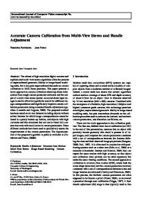
Figure 4: Images of the calibration pattern taken with different types of cameras. a) narrow-angle lens, b) wide-angle lens, c) fish-eye lens, d) hyperbolic mirror combined with a narrow-angle lens

References [1] J. Heikkil¨a, “Geometric camera calibration using circular control points,” IEEE Transactions on Pattern Analysis and Machine Intelligence, vol. 22, no. 10, pp. 1066–1077, 2000. [2] J. Kannala and S. S. Brandt, “A generic camera model and calibration method for conventional, wide-angle, and fish-eye lenses,” IEEE Transactions on Pattern Analysis and Machine Intelligence, vol. 28, no. 8, pp. 1335–1340, 2006. [3] A. Conrady, “Decentering lens systems,” Monthly notices of the Royal Astronomical Society, vol. 79, pp. 384–390, 1919. [4] D. C. Brown, “Close-range camera calibration,” Photogrammetric Engineering, vol. 37, no. 8, pp. 855–866, 1971. [5] C. C. Slama, Ed., Manual of Photogrammetry. Am. Soc. Photogrammetry, 1980. [6] R. Tsai, “A versatile camera calibration technique for high-accuracy 3D machine vision metrology using off-the-shelf TV cameras and lenses,” IEEE Journal of Robotics and Automation, vol. RA-3, no. 4, pp. 323–344, 1987. [7] O. Faugeras and Q.-T. Luong, The Geometry of Multiple Images. MIT Press, 2001. 18

The

[8] R. Hartley and A. Zisserman, Multiple View Geometry in Computer Vision, 2nd ed. Cambridge, 2003. [9] S. Baker and S. K. Nayar, “A theory of single-viewpoint catadioptric image formation,” International Journal of Computer Vision, vol. 35, no. 2, 1999. [10] C. Geyer and K. Daniilidis, “Catadioptric projective geometry,” International Journal of Computer Vision, vol. 45, no. 3, 2001. [11] X. Ying and Z. Hu, “Catadioptric camera calibration using geometric invariants,” IEEE Transactions on Pattern Analysis and Machine Intelligence, vol. 26, no. 10, 2004. [12] J. P. Barreto and H. Araujo, “Geometric properties of central catadioptric line images and their application in calibration,” IEEE Transactions on Pattern Analysis and Machine Intelligence, vol. 27, no. 8, pp. 1327–1333, 2005. [13] K. Miyamoto, “Fish eye lens,” Journal of the Optical Society of America, vol. 54, no. 8, pp. 1060–1061, 1964. [14] C. Br¨auer-Burchardt and K. Voss, “A new algorithm to correct fish-eyeand strong wide-angle-lens-distortion from single images,” in Proc. International Conference on Image Processing, 2001. [15] A. Fitzgibbon, “Simultaneous linear estimation of multiple view geometry and lens distortion,” in Proc. IEEE Conference on Computer Vision and Pattern Recognition, 2001. [16] B. Miˇcuˇs´ık and T. Pajdla, “Structure from motion with wide circular field of view cameras,” IEEE Transactions on Pattern Analysis and Machine Intelligence, vol. 28, no. 7, 2006. [17] R. Hartley and S. B. Kang, “Parameter-free radial distortion correction with center of distortion estimation,” IEEE Transactions on Pattern Analysis and Machine Intelligence, vol. 29, no. 8, pp. 1309–1321, 2008. [18] M. D. Grossberg and S. K. Nayar, “A general imaging model and a method for finding its parameters,” in Proc. International Conference on Computer Vision, 2001, pp. 108–115. [19] S. Ramalingam, “Generic Imaging Models: Calibration and 3D Reconstruction Algorithms,” Ph.D. dissertation, Institut National Polytechnique de Grenoble, 2006. [20] R. Swaminathan, M. D. Grossberg, and S. K. Nayar, “Designing mirror for catadioptric systems that minimize image errors,” in Proc. Workshop on Omnidirectional Vision, 2004. [21] J. S. Chahl and M. V. Srinivasan, “Reflective surfaces for panoramic imaging,” Applied Optics, vol. 36, no. 31, pp. 8275–8285, 1997. [22] M. Ollis, H. Herman, and S. Singh, “Analysis and design of panoramic stereo vision using equi-angular pixel cameras,” Carnegie Mellon University,” CMU-RI-TR-99-04, 1999. 19

[23] R. A. Hicks and R. K. Perline, “Equi-areal catadioptric sensors,” in Proc. Workshop on Omnidirectional Vision, 2002. [24] Z. Zhang, “A flexible new technique for camera calibration,” IEEE Transactions on Pattern Analysis and Machine Intelligence, vol. 22, no. 11, pp. 1330–1334, 2000. [25] Y. I. Abdel-Aziz and H. M. Karara, “Direct linear transformation from comparator to object space coordinates in close-range photogrammetry,” in Symposium on Close-Range Photogrammetry, 1971. [26] I. Sutherland, “Three-dimensional data input by tablet,” in Proc. IEEE, vol. 62, 1974, pp. 453–461. [27] P. Sturm and S. Maybank, “On plane based camera calibration: A general algorithm, singularities, applications,” in Proc. IEEE Conference on Computer Vision and Pattern Recognition, 1999, pp. 432–437. [28] J. Heikkil¨a and O. Silv´en, “Calibration procedure for short focal length off-the-shelf CCD cameras,” in Proc. International Conference on Pattern Recognition, 1996, pp. 166–170.

20