The Fourth IEEE RAS/EMBS International Conference on Biomedical Robotics and Biomechatronics Roma, Italy. June 24-27, 2012
Gait Segmentation Using Bipedal Foot Pressure Patterns S. M. M. De Rossi, S. Crea, M. Donati, P. Reberšek, D. Novak, N. Vitiello, T. Lenzi, J. Podobnik, M. Munih, M. C. Carrozza parameters of interest (e.g. the peak ground reaction force during push-off, or the peak pressure during the heel strike) requires additional sensors, most commonly a force plate. In this work, we propose an automated segmentation method based on the analysis of plantar pressure patterns recorded from two synchronized wireless foot insoles [1]. Our method uses a common machine-learning technique, Hidden Markov Models (HMMs, [10]), which has been widely applied to statistical pattern recognition in, e.g., voice recognition [22] and computer vision [21], as well as in gait segmentation [23] . Compared to other works (e.g. [16][23][18]), our method can segment the gait into an higher number (six) of phases, following a slightly simplified version of the classic gait model by Perry [6] with no swing-phase sub-division. Moreover, it does not require any subject-specific calibration or training, and requires a very simple signal pre-processing, making it potentially applicable on-line. The method has been tested on five healthy subjects at two different gait speeds.
Abstract— We present an automated gait segmentation method based on the analysis of foot plantar pressure patterns elaborated from two wireless pressure-sensitive insoles. The 64 pressure signals recorded by each device are elaborated to extract 10 feature variables which are used to segment the gait cycle into 6 sub-phases following a simplified version of Perry’s gait model. The method is based on a Hidden Markov Model with a minimum phase length constraint and a univariate Gaussian emission model, which is decoded using a classic Viterbi algorithm. The method is tested on a pool of 5 healthy young subjects walking at two different speeds, through a leave-one-out cross-subject validation. The results show that the method is highly effective, yielding to an average performance of about 95% of correct phase classification, and 85 to 90% of phase transitions detected inside an acceptance window of 50ms.
T
I. INTRODUCTION
HE detection of gait phases (gait segmentation) is a critical component of gait analysis, and is fundamental in a variety of fields, including clinical gait analysis and biomechanics [6][7][8][9]. Gait-phase related signals have been also proposed and applied as control variables for functional electrical stimulation treatments [16][17] and for active robotic prostheses [24]. In all these application fields, the development of automated methods to replace the human expert in performing the analysis of gait signals is of clear advantage. Several methods have been developed to automate this task, differing in terms of sensory systems, algorithms, and quality of the segmentation. A number of sensors has been proposed to perform gait segmentation, especially wearable sensors, including gyroscopes [16], accelerometers [17], force sensing resistors [16] and other force-contact sensors [18]. The clear advantage of low-encumbrance wearable systems is that of bringing gait analysis outside the laboratory environment [19], allowing long-period real-world measures. All methods allow to segment the gait in sub-phases, and therefore to compute temporal parameters [20] (e.g. the relative duration of the stance phase). The computation of other quantitative
II. MATERIALS AND METHODS A. Subjects and Protocol Five healthy young subjects (age: 28.8 ± 3.6) were chosen to span a wide range of body mass (weight 60-80 Kg, average 70.8 ± 7.4, height 172.8 ± 2.6 cm), with a similar shoe size (41.5-43 EU size). The subjects had no discernable gait abnormalities, and were comfortable in wearing the
Manuscript received January 15, 2012. This work was supported in part by the EU within the EVRYON Collaborative Project STREP (FP7-ICT2007-3-231451) and by the CYBERLEGs Project (FP7-ICT-2013-287894). S.M.M. De Rossi, S. Crea, M. Donati, N. Vitiello, T. Lenzi and M.C. Carrozza are with The BioRobotics Institute, Scuola Superiore Sant’Anna, viale Rinaldo Piaggio 34, Pontedera (PI), Italy. (S.M.M. De Rossi is corresponding author, phone: +39 050883472; e-mail:
[email protected]). P. Rebersek, D. Novak, J. Podobnik and M. Munih are with the Laboratory of Robotics, University of Ljubljana, Slovenia. 978-1-4577-1200-5/12/$26.00 ©2012 IEEE
Figure 1. Subject walking freely while wearing the instrumented shoes. 361
TABLE I SUBJECT CHARACTERISTICS Subject 1 2 3 4 5
Age [y] 34 31 27 27 25
Weight [Kg] 60 80 68 73 73
Height [cm] 176 171 175 172 170
Shoe Size [EU size] 41.5 41.5 43 42 42.5 (a)
equipment, which did not hinder their movements. Upon arrival, subjects wore comfortable sportswear and athletic shoes, equipped with an in-shoe pressure measurement system [1] (see Figure 1). Each subject was asked to walk on a straight line, starting from a still position at one end of the room, and ending at the opposite end. Subjects were instructed to walk at two different speeds: a normal pace and a fast pace, which were chosen freely by each subject. 100 steady-state steps were recorded for each walking speed, for a total of 200 steps for each subject, and 1000 steps in total. Transitory steps (such as initial and terminal steps) were not processed. The main characteristics of the subjects are summarized in Table I.
(b) Figure 2. Pressure sensitive insole used in the experiment. The device is shown (a) outside the shoe and (b) inside the shoe. In black, the array of pressure sensors covered by a silicone layer. In white, the housing for the processing and transmission electronics. Picture from [1].
D. Gait Segmentation The bipedal gait model used in this work divides the gait into six phases, summarized in Table II, which were defined as follows: - DS1: Bipedal support phase preceding right foot monopodal stance (left leg swing). This phase is comprised between the second peak of left foot vGRF (beginning of the left toe-off event) and the first peak of the right foot vGRF (end of right-foot heel strike). In this phase, left vGRF decreases to transfer support to the right foot, increasing right vGRF. - RS1: Right monopodal stance (1). This phase starts from the end of DS1, and concludes to the low peak of right vGRF. This phase is connected to the upward acceleration of the body, which unloads the supporting foot. - RS2: Right monopodal stance (2). This phase concludes the right stance (and left swing), from the end of RS1, to the second high peak of right vGRF. In this phase, the load is transferred to the tip of the right foot. - DS2: Bipedal support phase preceding left foot monopodal stance (right leg swing). - LS1, LS2 are equivalent to RS1 and RS2. The gait model employed in this work is a simplified version of the classic gait model by Perry [6], which divides each cycle into 8 phases (5 stance, 3 swing). A comparison of the two models, shown in Table II, highlights that our model is less specific in the segmentation of the swing phase, and that the RS1, RS2 (LS1, LS2) correspond only roughly to the midstance and terminal stance as defined in [6]. It can be also seen in Table II that each phase of our model determines the state of both legs. Based on these
B. Measurement System Two pressure-sensitive insoles were inserted in the shoes of the subject, in place of the regular insoles. This device (shown in Figure 2), preliminary presented in [1], is made of an array of 64 optoelectronic pressure sensors embedded in a layer of silicone. The sensor technology was presented in [2][3], and applied to measure a wide range of different loads. The sensor array measures the pressure over the plantar area (with the exception of the plantar arch), and transmits the data sampled at a 100Hz frequency, wirelessly to a remote data logging computer. This sensorized insoles can fit into a normal sneaker shoe of EU size 42. Foot sizes from 41 to 43 can fit comfortably in the instrumented shoe, which can run continuously for up to 7-8 hours with an on-board battery. The insoles require an off-line characterization [1], but no subject-specific calibration. C. Data Processing For each foot, the 64 voltage signals are converted into pressure values through a pre-computed calibration function (see [1]). A Laplacian surface smoothing algorithm [4][5] is applied to the pressure map to remove pressure outliers and regularize the surface. The pressure map is used to extract the values of vertical ground reaction force (vGRF), the position of the center of plantar pressures (CoPx, CoPy), and the partial ground reaction forces on the foot tip (vGRFt) and heel (vGRFh). For each insole, a total of 10 signals are considered, consisting on the 5 aforementioned variables and their firstorder time derivatives. All these aggregate values are of common interest in gait analysis and are classically employed to divide the gait into phases [6][7][8][9]. 362
TABLE II GAIT PHASES Our Model
Perry’s Model [6]
Symbol DS1 RS1 RS2 DS2 LS1 LS2
Right Foot Double Support (1) Right Stance (1) Right Stance (2) Double Support (2) Left stance (1) Left Stance (2)
Initial Contact, Loading Respose ~Midstance ~Terminal Stance Preswing Initial Swing, Midswing Midswing,, Terminal Swing
Left Foot Preswing Initial Swing, Midswing Midswing, Terminal Swing Initial Contact, Loading Respose ~Midstance ~Terminal Stance
definitions, the whole dataset was manually segmented by an expert who analyzed carefully the vGRF profiles, and marked the transitory events dividing each cycle into the six phases. An example segmentation is shown in Figure 3. E. Machine Learning Method Based on this analysis, we hypothesize that the observed signals (20, as defined previously) are modeled by a 6- states Hidden Markov Model (HMM) [10], with 20 observable states (emissions). Let 𝑺𝑺 = {𝑆𝑆𝑖𝑖 , 𝑖𝑖 = 1. .6} be the set of hidden states, corresponding to the set {DS1, RS1, RS2, DS2, LS1, LS2}, and 𝒁𝒁 = {𝑧𝑧1 , . . , 𝑧𝑧20 } the set of observable emissions. As shown in Figure 4, which represents the connections between gait phases, we chose a left-right cyclic model, which represents well the gait phase pattern during steadystate conditions. Only transitions to the next phase and selftransitions are allowed in this model. The underlying Markov Model is defined by a set of parameters 𝝀𝝀 = (𝝅𝝅, 𝑨𝑨, 𝑩𝑩), where 𝜋𝜋𝑖𝑖 = Pr [𝑋𝑋(𝑡𝑡0 ) = 𝑆𝑆𝑖𝑖 , 𝑖𝑖 = 1. .6] is the prior probability vector (probability of the Markov chain to occupy a certain state at 𝑡𝑡0 ), 𝑨𝑨 is the 6 × 6 state transition probability matrix, defined by 𝐴𝐴 = Pr�𝑋𝑋(𝑡𝑡𝑛𝑛+1 ) = 𝑆𝑆𝑗𝑗 � 𝑋𝑋(𝑡𝑡𝑛𝑛 ) = 𝑆𝑆𝑖𝑖 ] ⎧ 𝑖𝑖𝑖𝑖
Figure 3. Example of segmentation of a gait cycle in subphases made by the expert. On the two top panels, vertical ground reaction force from the right (top) and left (bottom) insoles. Three weight lines are put for reference, corresponding to 80%, 100% and 130% of the subject weight. On the bottom panel, the reference segmentation is shown, with transitions highlighted by a vertical line.
6
� 𝐴𝐴𝑖𝑖𝑖𝑖 = 1, ∀𝑗𝑗 ⎨ ⎩ 𝑖𝑖=1 and 𝑩𝑩 is the 20 × 6 emission matrix, which describes, for each state, a univariate Gaussian random variable of the emissions. In particular, 𝐵𝐵𝑖𝑖𝑖𝑖 = (𝜇𝜇𝑖𝑖𝑖𝑖 , 𝜎𝜎𝑗𝑗 ) where the contribution of the state 𝑗𝑗 to the emission 𝑧𝑧𝑖𝑖 is a random variable 𝒩𝒩(𝜇𝜇𝑖𝑖𝑖𝑖 , 𝜎𝜎𝑗𝑗 ). Following our choice of a leftright model, as depicted in Figure 4, the only allowed transitions (Aij > 0) are those to the same state Aii and to the subsequent state Aii +1 . Starting from the segmentation performed by the expert as described in Section II.D, each observed emission at time 𝑡𝑡 was labeled with a reference state 𝑆𝑆𝑟𝑟𝑟𝑟𝑟𝑟 (𝑡𝑡). The reference labeling was used partly to train the HMM, and partly to
363
evaluate the performances of the automated segmentation method. To keep the method simple, no input pre-processing was performed prior to the application of the HMM. In particular, no feature extraction, dimensionality reduction or frequency-space transforms were applied to the observed emissions 𝒁𝒁. Most importantly, no (subject-dependent) normalization was applied to the signals. The Leave-One-Out Cross-Subject Validation (LOOCV, see [10][11]) approach was applied to the training and validation of the method. In particular, data gathered from 𝑁𝑁 = 𝑄𝑄 − 1 = 4 subjects was used to train and optimize the HMM, while data from the remaining subject was used for validation. LOOCV was applied five times to all possible subject subsets to test the generalization capabilities of the method. For each repetition of the LOOCV, the union of the datasets of the 𝑁𝑁 training subjects makes up the training dataset (800 gait cycles), while the remaining data makes up the testing dataset (200 gait cycles). The model parameters 𝝀𝝀 were estimated from the training dataset through a simple statistical estimation method. The transition matrix elements 𝐴𝐴𝑖𝑖𝑖𝑖 were calculated as 𝑇𝑇𝑖𝑖𝑖𝑖 𝐴𝐴𝑖𝑖𝑖𝑖 = 𝑁𝑁𝑖𝑖 were 𝑇𝑇𝑖𝑖𝑖𝑖 is the number of samples of the training dataset with a transition from state 𝑆𝑆𝑖𝑖 to state 𝑆𝑆𝑗𝑗 , and 𝑁𝑁𝑖𝑖 is the total number of samples labeled with state 𝑆𝑆𝑖𝑖 . The elements of
this, the precision of the method was evaluated by computing the number of transitions detected inside the acceptance window. To evaluate the performance of the algorithm at different walking speeds, the entire dataset was also split into a fast gait dataset, and a normal gait dataset. All the performance indices were computed on the testing dataset as a whole, and on the fast and normal datasets separately. Figure 4. Hidden Markov Model representing the phases of a gait cycle. Each state of the Markov Model is identified by a circled label, and allowed state transitions are marked by an arrow. A sketch of the human represents each phase (the right leg is highlighted in grey). Sketches are adapted from [14].
emission matrix 𝑩𝑩 were computed by respectively the sample mean and sample standard deviation of the emissions in each state. The prior probability vector was set to 𝝅𝝅 = (1, 0, 0, 0, 0, 0) to represent the known state DS1 from which all observation started. The HMM structure was fixed to a six-state left-right model (Figure 4), therefore no structure estimation algorithm (like the Baum-Welch algorithm [13]) was required. Testing of the method was done using the Viterbi decoding algorithm [15], which estimates the most likely state 𝑆𝑆𝑒𝑒𝑒𝑒𝑒𝑒 (𝑡𝑡) based on the previous estimation 𝑆𝑆𝑒𝑒𝑒𝑒𝑒𝑒 (𝑡𝑡 − 1) and current observable emissions 𝒁𝒁(𝑡𝑡). The Viterbi algorithm was run on the entire testing dataset, and the estimated labeling was then compared to the reference to evaluate its performances. A common problem when using the Viterbi algorithm in left-right HMMs is that of deletions and insertions [11], consisting respectively in missed detections of full gait cycles, and erroneous insertion of quick cycles when no transitions should have been detected. A simple solution to this problem is that of imposing a minimal duration to each state (phase) 𝑆𝑆𝑖𝑖 . Transitions which are decoded before the minimum phase length are rejected, and the estimated state 𝑆𝑆𝑒𝑒𝑒𝑒𝑒𝑒 (𝑡𝑡) is kept to the original value 𝑆𝑆𝑒𝑒𝑒𝑒𝑒𝑒 (𝑡𝑡 − 1). The minimal duration vector was estimated starting from the average duration of each phase in the whole training dataset, and was set to half of the mean value, to encompass all the variability in the duration of gait phases across subjects. Implementation of the HMMs, of the Baum-Welch and of the Viterbi decoding algorithms were done using MATLAB® by Mathworks, and the HMM toolbox [12].
III. RESULTS Table III reports the steps cadence in the normal and fast gait datasets. The average step cadence (across all subjects) was 0.85 ± 0.08 Hz (102 ± 10 steps/min) for the normal gait, and 1.06 ± 0.05 Hz (127 ± 6 steps/min) for the fast gait, for an average of 0.96 ± 0.07 Hz (115 ± 8 steps/min). Cadence was computed as the inverse of the duration of a complete gait cycle. Figure 5 shows an example run of the Viterbi decoder on the HMM model, on the data of three steps (normal walking speed). For the sake of simplicity, only a subset of 3 of the 20 variables is shown, along with the reference and the estimated gait phase. Table IV presents the classification performances of the automated algorithm in terms of percentage of correct estimates. Results are shown for the entire testing set, and for the normal and fast gait dataset separately. Each row of the table corresponds to the HMM being trained on the whole dataset (normal and fast) from 4 out of 5 subjects, and tested on the remaining subject normal, fast and whole datasets. Figures are also reported averaged across all subjects. Table V shows the fraction of phase transitions detected by the algorithm inside a 50ms window about the reference transition. Results are shown for each testing subject and each of the 6 transitions, and averaged across all subjects. No insertions nor deletions were present after the Viterbi algorithm was run, thanks to the minimum duration constraint included in the decoder. IV. DISCUSSION The overall performance shown by our method in Table IV denotes an high specificity in the capacity to segment and classify the gait cycle into sub-phases. The average performance of 96% right classification (with a minimum of 93% and a maximum of 97%) corresponds roughly to 6 wrong samples for each gait cycle. This performances are in line with state-of-the-art methods, both using rule-based approaches [16], or machine learning methods [23][25][29]. This is particularly remarkable in light of the higher complexity of the model employed in our algorithm, which includes 6 gait phases (equivalent to Perry’s [6] standard model, with no swing segmentation), instead of four [23][16] or less [26][27]. Comparable performance holds when looking at the datasets split by gait pace. However, it can be seen that the method is less performing in slower gait (average 93%), than in fast gait (average 98.5%). This could be in part explained
F. Evaluation of Performances The performance of the algorithm was evaluated with the LOOCV method based on two performance indices. On one side, we computed the percentage of right (and wrong) classifications 𝑛𝑛, as #(𝑆𝑆𝑒𝑒𝑒𝑒𝑒𝑒 (𝑡𝑡) = 𝑆𝑆𝑟𝑟𝑟𝑟𝑟𝑟 (𝑡𝑡)) 𝑛𝑛 = #𝑆𝑆𝑟𝑟𝑟𝑟𝑟𝑟 (𝑡𝑡) The performance 𝑛𝑛 was computed over the whole dataset, outside of a tolerance window of 5 samples (50ms) about each reference transition. The tolerance window accounts for a minimal discretionary variability in the estimate, which is also present in the segmentation by the expert. In addition to 364
TABLE III GAIT CADENCE Subj ect 1 2 3 4 5 Avg.
Normal Gait Cadence [𝜇𝜇 ± 𝜎𝜎, Hz] 0.89 ± 0.07 0.83 ± 0.09 0.86 ± 0.08 0.86 ± 0.08 0.82 ± 0.09 0.85 ± 0.08
Fast Gait Cadence [𝜇𝜇 ± 𝜎𝜎, Hz] 1.12 ± 0.08 1.07 ± 0.05 1.04 ± 0.03 1.02 ± 0.02 1.07 ± 0.05 1.06 ± 0.05
Average Cadence [𝜇𝜇 ± 𝜎𝜎, Hz] 1.01 ± 0.08 0.95 ± 0.08 0.95 ± 0.06 0.94 ± 0.05 0.95 ± 0.07 0.96 ± 0.07
TABLE IV PERCENTAGE OF RIGHT (WRONG) CLASSIFICATION IN THE TESTING SETS Subject
Normal Gait [%]
Fast Gait [%]
All gait cycles [%]
1 2 3 4 5 Avg.
94.8 (5.2) 90.3 (9.7) 88.3 (11.7) 94.4 (5.6) 95.1 (4.9) 92.6 (7.4)
97.9 (2.1) 99.2 (0.8) 97.5 (2.5) 99.8 (0.2) 98.3 (1.7) 98.5 (1.5)
96.4 (3.6) 94.8 (5.2) 92.9 (7.1) 97.1 (2.9) 96.7 (3.3) 95.6 (4.4)
TABLE V PERCENTAGE OF TRANSITIONS INSIDE THE TOLERANCE WINDOW State (Phase) Transitions Subj ect 1 2 3 4 5 Avg.
S1→ S2
S2→ S3
S3→ S4
S4→ S5
S5→ S6
S6→ S1
90.5 75.6 92.5 93.2 89.2 88.2
90.9 87.8 66.9 48.4 70.7 72.9
90.5 74.5 77.0 97.1 92.6 86.3
85.2 97.1 81.5 98.4 89.3 90.3
93.9 91.9 67.5 86.5 91.3 86.2
92.1 90.8 76.0 89.0 97.1 89.0
Figure 5. Example results of the Viterbi decoder compared to the segmentation by an expert. On the top panels, three representative observed variables (vGRF, CoPY and CoPY’) are shown for the right foot. CoP values are shown only during the stance phase. On the bottom panel the solid line shows the reference segmentation, the dashed line the output of our algorithm.
generalization capabilities by the HMM in relation to this event. The worst-case performances, both in terms of worstperforming subject (number 2), and worst-performing transition, are not satisfactory, thus requiring further investigations to increase the reliability of the method. Compared to similar machine-learning based methods (e.g. [27][25][29]), this algorithm requires no subjectdependent calibration, and, most importantly, a very simple data pre-processing, with no need of frequency-space transforms or dimensionality reduction. This characteristics, together with the use of the Viterbi algorithm, make this method potentially applicable to an on-line phase estimation, alike rule-based methods [16][28]. This could extend the applicability of this method to FES or robot prostheses control. On top of this, a field of applicability of this method is that of quantitative gait analysis (for both medical or biomechanical purposes) outside of the laboratory environment. We used a wireless pressure-measurement insole with long autonomy to segment the gait. Our method therefore could allow not only to evaluate temporal gait parameters (e.g. relative duration of the stance or sub-stance phases) but also kinetic parameters (e.g. peak vGRF during push-off) using the same wearable sensory system.
by the different walking pattern during fast gait (which includes sharper transitions and force peaks), and also by the higher relative width of tolerance windows in steps of shorter duration. In all cases however, it is clear after the LOOCV that the method generalizes to different subjects with highly variable body characteristics (see Table I). This is interesting since the method does not require a subject-specific calibration, and is shown to work well even when tested with subjects of very different weight compared to the average of the dataset (see e.g. subject 2). In terms of precision in the detection of transitions, it can be seen that, with the exception of one subject, an average 85 to 90% of events are detected inside the 50ms tolerance window about each reference transition. This is in line with other works using pressure insoles, like [26][29]. A closer look to results in Table V shows however that some transitions are detected with much less precision, reaching a lowest value of less than 50% of 𝑆𝑆2 → 𝑆𝑆3 transitions detected inside the window, and a very low average value for the same transition across subjects. This is determined in particular by subject 3 and 4, and reflects to the ‘twin’ transition S5→ S6, at least for subject 3, suggesting lesser 365
V. CONCLUSION
[15] Forney, G. D. (1973). The viterbi algorithm. Proceedings of the IEEE, 61(3), 268-278. [16] Pappas, I. P., Popovic, M. R., Keller, T., Dietz, V., & Morari, M. (2001). A reliable gait phase detection system. IEEE transactions on neural systems and rehabilitation engineering, 9(2), 113-25. [17] Williamson, R., & Andrews, B. J. (2000). Gait event detection for FES using accelerometers and supervised machine learning. IEEE transactions on rehabilitation engineering, 8(3), 312-9. [18] Kong, K., & Tomizuka, M. (2009). A Gait Monitoring System Based on Air Pressure Sensors Embedded in a Shoe. IEEE/ASME Transactions on Mechatronics, 14(3), 358-370. [19] Bamberg, S. J. M., Benbasat, A. Y., Scarborough, D. M., Krebs, D. E., & Paradiso, J. A. (2008). Gait analysis using a shoe-integrated wireless sensor system. IEEE transactions on information technology in biomedicine, 12(4), 413-23. [20] Wall, J. C., & Crosbie, J. (1996). Accuracy and reliability of temporal gait measurement. Gait & Posture, 4, 293-296. [21] Wilson, A. D., & Bobick, A. F. (1999). Parametric hidden Markov models for gesture recognition. IEEE Transactions on Pattern Analysis and Machine Intelligence, 21(9), 884-900. [22] Rabiner, L. R. (1989). A tutorial on hidden Markov models and selected applications in speech recognition. Proceedings of the IEEE, 77(2), 257-286. doi:10.1109/5.18626 [23] Mannini, A., & Sabatini, A. M. (2011). A hidden Markov modelbased technique for gait segmentation using a foot-mounted gyroscope. 2011 Annual International Conference of the IEEE Engineering in Medicine and Biology Society (pp. 4369-4373). [24] Au, S., Berniker, M., & Herr, H. (2008). Powered ankle-foot prosthesis to assist level-ground and stair-descent gaits. Neural Networks, 21(4), 654-666. [25] Kirkwood, C. A., Andrews, B. J., & Mowforth, P. (1989). Automatic detection of gait events: a case study using inductive learning techniques. Journal of biomedical engineering, 11(6), 511-6. [26] Detection of gait events using an F-Scan in-shoe pressure measurement system 10.1016/j.gaitpost.2008.01.019 : Gait & Posture [27] Miller, A. (2009). Gait event detection using a multilayer neural network. Gait & posture, 29(4), 542-5. [28] Kong, K., & Tomizuka, M. (2008). Smooth and continuous human gait phase detection based on foot pressure patterns. 2008 IEEE International Conference on Robotics and Automation, 3678-3683. [29] Huang, B., Chen, M., Shi, X., & Xu, Y. (2007). Gait Event Detection with Intelligent Shoes. 2007 International Conference on Information Acquisition (pp. 579-584).
We presented an automated gait segmentation method based on the analysis of foot plantar pressure patterns elaborated from two wireless pressure-sensitive insoles. The method requires simple pre-processing of the signal data, no subject-specific calibration, and uses the straightforward Viterbi HMM state decoding algorithm. Consequently, the method could be easily applied on-line. The method performed well on average on the pool of subjects, leading to classification performances close to 95%. 85 to 90% of phase transitions were detected inside an acceptance window of 50 ms, with the exception of one subject. For some specific phase transitions (and in a subject-dependent way), the method underperformed, reaching, in the worst case, a performance of 70% transition events detected inside the acceptance window. Future works will be aimed at increasing the performances of the algorithm, especially in the worst case scenarios. More elaborate pre-processing techniques will be investigated, such as the application of feature-extraction methods to the raw input, relative normalization of the data, and frequency-transform techniques. REFERENCES [1]
[2]
[3]
[4] [5] [6] [7] [8] [9] [10] [11] [12] [13]
[14]
S. M. M. De Rossi et al., “Development of an in-shoe pressuresensitive device for gait analysis,” in Engineering in Medicine and Biology Society (EMBC), 2011 Annual International Conference of the IEEE, 2011, pp. 5637-5640. De Rossi, S. M. M., Vitiello, N., Lenzi, T., Ronsse, R., Koopman, B., Persichetti, A., Vecchi, F., et al. (2010). Sensing Pressure Distribution on a Lower-Limb Exoskeleton Physical Human-Machine Interface. Sensors, 11(1), 207–227. Lenzi, T., Vitiello, N., De Rossi, S. M. M., Persichetti, A., Giovacchini, F., Roccella, S., Vecchi, F., et al. (2011). Measuring human–robot interaction on wearable robots: A distributed approach. Mechatronics, 21, 1123-1131. Elsevier Ltd. Field, D. A. (1988). Laplacian smoothing and Delaunay triangulations. Communications in Applied Numerical Methods, 4(6), 709-712. Lo, S. H. (1985). A new mesh generation scheme for arbitrary planar domains. International Journal for Numerical Methods in Engineering, 21(8), 1403-1426. Perry, J. (1992). Gait Analysis: Normal and Pathological Function. Journal of Pediatric Orthopaedics (Vol. 12, p. 815). Slack Incorporated. doi:10.1001 Cornwall, M., & McPoil, T. (2000). Velocity of the center of pressure during walking. J Am Podiatr Med Assoc, 90(7), 334-338. Townsend, M. A. (1985). Biped gait stabilization via foot placement. Journal of biomechanics, 18(1), 21-38. Winter, D. A. (1992). Foot trajectory in human gait: a precise and multifactorial motor control task. Physical therapy, 72(1), 45-53; discussion 54-6. Devijver, P. A., & Kittler, J. (1982). Pattern recognition: A statistical approach (p. 448). Prentice/Hall International. Geisser, S. (1993). Predictive inference: an introduction (p. 264). Chapman & Hall. Murphy, K. (1998). Hidden Markov Model (HMM) Toolbox for Matlab. http://www.cs.ubc.ca/~murphyk/Software/HMM/hmm.html Baum, L. E., Petrie, T., Soules, G., & Weiss, N. (1970). A maximization technique occurring in the statistical analysis of probabilistic functions of Markov chains. The Annals of Mathematical Statistics, 41(1), 164-171. Thompson, D. (2002). Introduction to the study of human walking. http://moon.ouhsc.edu/dthompso/gait/intro.htm
366