11 Fuzzy Logic

11.1 Fuzzy sets and fuzzy logic We showed in the last chapter that the learning problem is NP-complete for a broad class of neural networks. Learning algorithms may require an exponential number of iterations with respect to the number of weights until a solution to a learning task is found. A second important point is that in backpropagation networks, the individual units perform computations more general than simple threshold logic. Since the output of the units is not limited to the values 0 and 1, giving an interpretation of the computation performed by the network is not so easy. The network acts like a black box by computing a statistically sound approximation to a function known only from a training set. In many applications an interpretation of the output is necessary or desirable. In all such cases the methods of fuzzy logic can be used. 11.1.1 Imprecise data and imprecise rules Fuzzy logic can be conceptualized as a generalization of classical logic. Modern fuzzy logic was developed by Lotfi Zadeh in the mid-1960s to model those problems in which imprecise data must be used or in which the rules of inference are formulated in a very general way making use of diffuse categories [170]. In fuzzy logic, which is also sometimes called diffuse logic, there are not just two alternatives but a whole continuum of truth values for logical propositions. A proposition A can have the truth value 0.4 and its complement Ac the truth value 0.5. According to the type of negation operator that is used, the two truth values must not be necessarily add up to 1. Fuzzy logic has a weak connection to probability theory. Probabilistic methods that deal with imprecise knowledge are formulated in the Bayesian framework [327], but fuzzy logic does not need to be justified using a probabilistic approach. The common route is to generalize the findings of multivalued logic in such a way as to preserve part of the algebraic structure [62]. In

R. Rojas: Neural Networks, Springer-Verlag, Berlin, 1996

290

11 Fuzzy Logic

this chapter we will show that there is a strong link between set theory, logic, and geometry. A fuzzy set theory corresponds to fuzzy logic and the semantic of fuzzy operators can be understood using a geometric model. The geometric visualization of fuzzy logic will give us a hint as to the possible connection with neural networks. Fuzzy logic can be used as an interpretation model for the properties of neural networks, as well as for giving a more precise description of their performance. We will show that fuzzy operators can be conceived as generalized output functions of computing units. Fuzzy logic can also be used to specify networks directly without having to apply a learning algorithm. An expert in a certain field can sometimes produce a simple set of control rules for a dynamical system with less effort than the work involved in training a neural network. A classical example proposed by Zadeh to the neural network community is developing a system to park a car. It is straightforward to formulate a set of fuzzy rules for this task, but it is not immediately obvious how to build a network to do the same nor how to train it. Fuzzy logic is now being used in many products of industrial and consumer electronics for which a good control system is sufficient and where the question of optimal control does not necessarily arise. 11.1.2 The fuzzy set concept The difference between crisp (i.e., classical) and fuzzy sets is established by introducing a membership function. Consider a finite set X = {x1 , x2 , . . . , xn } which will be considered the universal set in what follows. The subset A of X consisting of the single element x1 can be described by the n-dimensional membership vector Z(A) = (1, 0, 0, . . . , 0), where the convention has been adopted that a 1 at the i-th position indicates that xi belongs to A. The set B composed of the elements x1 and xn is described by the vector Z(B) = (1, 0, 0, ..., 1). Any other crisp subset of X can be represented in the same way by an n-dimensional binary vector. But what happens if we lift the restriction to binary vectors? In that case we can define the fuzzy set C with the following vector description: Z(C) = (0.5, 0, 0, ..., 0) In classical set theory such a set cannot be defined. An element belongs to a subset or it does not. In the theory of fuzzy sets we make a generalization and allow descriptions of this type. In our example the element x1 belongs to the set C only to some extent. The degree of membership is expressed by a real number in the interval [0, 1], in this case 0.5. This interpretation of the degree of membership is similar to the meaning we assign to statements such as “person x1 is an adult”. Obviously, it is not possible to define a definite age which represents the absolute threshold to enter into adulthood. The act of becoming mature can be interpreted as a continuous process in which the membership of a person to the set of adults goes slowly from 0 to 1.

R. Rojas: Neural Networks, Springer-Verlag, Berlin, 1996

11.1 Fuzzy sets and fuzzy logic

291

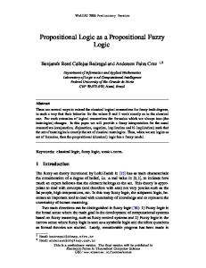
There are many other examples of such diffuse statements. The concepts “old” and “young” or the adjectives “fast” and “slow” are imprecise but easy to interpret in a given context. In some applications, such as expert systems, for example, it is necessary to introduce formal methods capable of dealing with such expressions so that a computer using rigid Boolean logic can still process them. This is what the theory of fuzzy sets and fuzzy logic tries to accomplish. 1

young

mature

0.8 old degree of membership

0.2 0 10

20

30

40

50

60

70

age

Fig. 11.1. Membership functions for the concepts young, mature and old

Figure 11.1 shows three examples of a membership function in the interval 0 to 70 years. The three functions define the degree of membership of any given age in the sets of young, adult, and old ages. If someone is 20 years old, for example, his degree of membership in the set of young persons is 1.0, in the set of adults 0.35, and in the set of old persons 0.0. If someone is 50 years old the degrees of membership are 0.0, 1.0, 0.3 in the respective sets. Definition 11. Let X be a classical universal set. A real function μA : X → [0, 1] is called the membership function of A and defines the fuzzy set A of X. This is the set of all pairs (x, μA (x)) with x ∈ X. A fuzzy set is completely determined by its membership function. Note that the above definition also covers the case in which X is not a finite set. The set of support of a fuzzy set A is the set of all elements x of X for which (x, μA (x)) ∈ A and μA (x) > 0 holds. A fuzzy set A with the finite set of support {a1 , a2 , . . . , am } can be described in the following way A = μ1 /a1 + μ2 /a2 + · · · + μm /am , where μi = μA (ai ) for i = 1, . . . , m. The symbols “/” and “+” are used only as syntactical constructors.

R. Rojas: Neural Networks, Springer-Verlag, Berlin, 1996

292

11 Fuzzy Logic

Crisp sets are a special case of fuzzy sets, since the range of the function is restricted to the values 0 and 1. Operations defined over crisp sets, such as union or intersection, can be generalized to cover also fuzzy sets. Assume as an example that X = {x1 , x2 , x3 }. The classical subsets A = {x1 , x2 } and B = {x2 , x3 } can be represented as A = 1/x1 + 1/x2 + 0/x3

B = 0/x1 + 1/x2 + 1/x3 .

The union of A and B is computed by taking for each element xi the maximum of its membership in both sets, that is: A ∪ B = 1/x1 + 1/x2 + 1/x3 The fuzzy union of two fuzzy sets can be computed in the same way. The union of the two fuzzy sets C = 0.5/x1 + 0.6/x2 + 0.3/x3

D = 0.7/x1 + 0.2/x2 + 0.8/x3

is given by C ∪ D = 0.7/x1 + 0.6/x2 + 0.8/x3 The fuzzy intersection of two sets A and B can be defined in a similar way, but instead of taking the maximum we compute the minimum of the membership of each element xi to A and B. The maximum or minimum of the membership values are just one pair of possible definitions of the union and intersection operations for fuzzy sets. As we show later on, there are other alternative definitions. 11.1.3 Geometric representation of fuzzy sets Bart Kosko introduced a very useful graphical representation of fuzzy sets [259]. Figure 11.2 shows an example in which the universal set consists only of the two elements x1 and x2 . Each point in the interior of the unit square represents a subset of X. The convention is that the coordinates of the representation correspond to the membership values of the elements in the fuzzy set. The point (1, 1), for example, represents the universal set X, with membership function μA (x1 ) = 1 and μA (x2 ) = 1. The point (1, 0) represents the set {x1 } and the point (0, 1) the set {x2 }. The crisp subsets of X are located at the vertices of the unit square. The geometric visualization can be extended to an n-dimensional hypercube. Kosko calls the inner region of a unit hypercube in an n-dimensional space the fuzzy region. We find here all combinations of membership values that a fuzzy set could assume. The point M in Figure 11.2 corresponds to the fuzzy set M = 0.5/x1 + 0.3/x2 . The center of the square represents the most diffuse of all possible fuzzy sets of X, that is the set Y = 0.5/x1 + 0.5/x2 . The degree of fuzziness of a fuzzy set can be measured by its entropy. In the geometric visualization, this corresponds inversely to the distance between

R. Rojas: Neural Networks, Springer-Verlag, Berlin, 1996

11.1 Fuzzy sets and fuzzy logic {x } = (0,1)

293

X = (1,1)

2

Y

0,5

M 0,3

∅ = (0,0)

{x 1} = (1,0)

0,5

Fig. 11.2. Geometric visualization of fuzzy sets

the representation of the set and the center of the unit square. The set Y in Figure 11.3 has the maximum possible entropy. The vertices represent the crisp sets and have the lowest entropy, that is, zero. Note that the fuzzy concept of entropy is mathematically different from the entropy concept in physics or information theory. Some authors prefer to use terms like index of fuzziness [239] or also crispness, certitude, ambiguity, etc. [55]. With this caveat we adopt a preliminary definition of the entropy of a fuzzy set M as the quotient of the distance d1 (according to some metric) of the corner which is nearest to the representation of M to the distance d2 from the corner which is farthest away. Figure 11.3 shows the two relevant segments. The entropy E(M ) of M is therefore E(M ) =

d1 . d2

According to this definition the entropy is bounded by 0 and 1. The maximum entropy is reached at the center of the square. The union or intersection of sets can be also visualized using this representation. The membership function for the the union of two sets A and B can be defined as μA∪B (x) = max(μA (x), μB (x)) ∀x ∈ X

(11.1)

and corresponds to the maximum of the corresponding coordinates in the geometric visualization. The membership function for the intersection of two sets A and B is given by μA∩B (x) = min(μA (x), μB (x)) ∀x ∈ X.

(11.2)

Together with the points representing the sets A and B, Figure 11.4 shows the points which represent their union and intersection.

R. Rojas: Neural Networks, Springer-Verlag, Berlin, 1996

294

11 Fuzzy Logic {x 2} = (0,1)

X = (1,1)

d2 M 1/3

d1 ∅ = (0,0)

{x 1} = (1,0)

1/2

Fig. 11.3. Distance of the set M to the universal and to the void set {x 2} = (0,1)

X = (1,1)

A

A∪B

B

A∩B ∅ = (0,0)

{x 1} = (1,0)

Fig. 11.4. Intersection and union of two fuzzy sets

The union or intersection of two fuzzy sets is in general a fuzzy, not a crisp set. The complement Ac of a fuzzy set A can be defined with the help of the membership function μAc given by μAc (x) = 1 − μA (x) ∀x ∈ X .

(11.3)

Figure 11.5 shows that the representation of A must be transformed into another point at the same distance from the center of the unit square. The line joining the representation of A and Ac goes through the center of the square. Figure 11.5 also shows how to obtain the representations for A ∪ Ac and A ∩ Ac using the union and intersection operators defined before. For fuzzy sets, it holds in general that A ∪ Ac = X

and

A ∩ Ac = ∅

which is not true in classical set theory. This means that the principle of excluded middle and absence of contradiction do not necessarily hold in fuzzy logic. The consequences will be discussed later.

R. Rojas: Neural Networks, Springer-Verlag, Berlin, 1996

11.1 Fuzzy sets and fuzzy logic

{x 2} = (0,1)

295

X = (1,1) c A∪A

A

A∩A

Ac

c

∅ = (0,0)

{x 1} = (1,0)

Fig. 11.5. Complement Ac of a fuzzy set

Kosko [259] establishes a direct relationship between the entropy of fuzzy sets and the geometric visualization of the union and intersection operations. To compute the entropy of a set, we need to determine the distance between the origin and the coordinates of the set. This distance is called the cardinality of the fuzzy set. Definition 12. Let A be a subset of a universal set X. The cardinality |A| of A is the sum of the membership values of all elements of X with respect to A, i.e.,  |A| = μA (x) x∈X

This definition of cardinality corresponds to the distance of the representation of A from the origin using a Manhattan metric. Figure 11.6 shows how to define the entropy of a set A using the cardinality of the sets A ∩ Ac and A ∪ Ac . The Manhattan distances d1 and d2 , introduced before to measure the fuzzy entropy, correspond to the cardinalities of the sets A ∩ Ac and A ∪ Ac . The entropy concept introduced previously in an informal manner can then be formalized with our next definition. Definition 13. The real value E(A) =

|A ∩ Ac | |A ∪ Ac |

is called the entropy of the fuzzy set A. The entropy of a crisp set is always zero, since for a crisp set A ∩ Ac = ∅. In fuzzy set theory E(A) is a value in the interval [0, 1], since A ∩ Ac can be non-void. Some authors take the geometric definition of entropy as given and derive Definition 13 as a theorem, which is called the fuzzy entropy theorem. [259]. Here we take the definition as given, since the geometric interpretation of fuzzy union and intersection depends on the exact definition of the fuzzy operators.

R. Rojas: Neural Networks, Springer-Verlag, Berlin, 1996

296

11 Fuzzy Logic {x 2} = (0,1)

X = (1,1) d1

A

A∪A

d2

d2 A∩A

∅ = (0,0)

d1

c

c Ac {x 1} = (1,0)

Fig. 11.6. Geometric representation of the entropy of a fuzzy set

11.1.4 Fuzzy set theory, logic operators, and geometry It is known in mathematics that an isomorphism exists between set theory and classic propositional logic. In set theory, the three operators union, intersection, and complement (∪, ∩, c) allow the construction of new sets from other sets. In propositional logic, the operators OR, AND and NOT (∨, ∧, ¬) are used to build new propositions. The union operator of classical set theory can be constructed using the OR operator. Let A and B be two crisp sets, that is, μA , μB : X → {0, 1}. The membership function μa∪B of the union set A ∪ B is μA∪B (x) = μA (x) ∨ μB (x)

∀x ∈ X ,

(11.4)

where the value 0 is interpreted as the logic value false and 1 as true. In a similar way it holds that for the intersection of the sets A and B μA∩B (x) = μA (x) ∧ μB (x)

∀x ∈ X.

(11.5)

For the complement Ac of the set A it holds that μAc (x) = ¬μA (x)

(11.6)

This correspondence between the operators of classical set theory and classical logic can be extended to the validity of some equations in both systems. The laws of de Morgan, for example, are valid in classical set theory as well as in classical logic: (A ∪ B)c ≡ Ac ∩ B c

corresponds to

¬(A ∨ B) ≡ ¬A ∧ ¬B

(A ∩ B)c ≡ Ac ∪ B c

corresponds to

¬(A ∧ B) ≡ ¬A ∨ ¬B

A fuzzy logic can be also derived from fuzzy set theory by respecting the isomorphism mentioned above. The fuzzy AND, OR, and NOT operators must

R. Rojas: Neural Networks, Springer-Verlag, Berlin, 1996

11.1 Fuzzy sets and fuzzy logic

297

be defined in such a way that the same general kinds of relation exist between them and their equivalents in classical set theory and logic. The straightforward approach is therefore to identify the OR operation ˜ ) with the maximum function, AND (∧ ˜ ) with the minimum, and comple(∨ mentation (˜ ¬) with the function x → 1 − x. Equations (11.1), (11.2), and (11.3) can be written as ˜ μB (x) μA∪B (x) = μA (x) ∨ ˜ μB (x) μA∪B (x) = μA (x) ∨ ˜ μA (x) μAc (x) = ¬

∀x ∈ X ∀x ∈ X

∀x ∈ X

(11.7) (11.8) (11.9)

In this way an isomorphism between fuzzy set theory and fuzzy logic is constructed which preserves the properties of the isomorphism present in the classical theories. Many rules of classical logic are still valid in the world of fuzzy operators. For example, the functions min and max are commutative and associative. However, the principle of no contradiction has been abolished. For a proposition A with truth value 0.4 we get ˜¬ A∧ ˜ A = min(0.4, 1 − 0.4) = 0 The principle of excluded middle is not valid for A either: ˜¬ A∨ ˜ A = max(0.4, 1 − 0.4) = 1 11.1.5 Families of fuzzy operators Up to this point we have worked with fuzzy operators defined in a rather informal way, since there are whole families of these operators that can be defined. Now we will give an axiomatic definition using the properties we would like the operators to exhibit. Consider the fuzzy OR operator. In the fuzzy logic literature [248] such an operator is required to fulfill the following axioms: •

Axiom U1. Boundary conditions: ˜0=0 0∨ ˜0=1 1∨ ˜1=1 0∨ ˜1=1 1∨

•

Axiom U2. Commutativity: ˜ b=b∨ ˜a a∨

•

Axiom U3. Monotonicity:

R. Rojas: Neural Networks, Springer-Verlag, Berlin, 1996

298

11 Fuzzy Logic

˜ b . ˜ b ≤ a ∨ If a ≤ a and b ≤ b , then a ∨ •

Axiom U4. Associativity: ˜ (b ∨ ˜ c) = (a ∨ ˜ b) ∨ ˜c a∨

It is easy to show that the maximum function fulfills these four conditions. There are many other functions for which the four axioms are valid, for example B(a, b) = min(1, a + b) which is called the bounded sum of a and b. An alternative fuzzy OR operator can be defined using this function. However, the bounded sum is not idempotent, that is, in general B(a, a) = a. We can therefore introduce a fifth axiom to exclude such operators: •

Axiom U5. Idempotence: ˜a=a a∨

Depending on the axioms selected, different fuzzy operators and different logic systems can be defined. Consequently, the term fuzzy logic refers to a family of different theories and not to a unique system of logic. ˜ axioms are also formulated in such a way In the case of the fuzzy operator ∧ that fuzzy AND is monotonic, commutative, and associative. The boundary conditions are: ˜0= 0∧ ˜0= 1∧ ˜1= 0∧ ˜1= 1∧

0 0 0 1

Idempotence can be demanded and can be enforced using a fifth axiom. For the fuzzy negation we use the following three axioms: •

Axiom N1. Boundary conditions: ¬ ˜1 = 0 ¬ ˜0 = 1

•

Axiom N2. Monotonicity: If a ≤ b then ¬ ˜b ≤ ¬ ˜ a.

•

Axiom N3. Involution: ¬ ˜¬ ˜a = a

R. Rojas: Neural Networks, Springer-Verlag, Berlin, 1996

11.1 Fuzzy sets and fuzzy logic max(x,y)

min(x,y)

1

1

0.75 .75

0.75 .75

0.5

0.5

0.25 .25

0.25 .25

0 1

0.8 0.8

0.6

1

0 1

0.6 0.4

y

0.4 0.2

299

0.2

0.8 0.8

x

0.6

0.6 0.4

y

0

1

0.4 0.2

0.2

x

0

Fig. 11.7. The max and min functions

The difference between these fuzzy operators can be better visualized by looking at their graphs. Figure 11.7 shows the graphs of the functions max and min, that is, a possible fuzzy AND and fuzzy OR combination. They could also be used as activation functions in neural networks. Using output functions derived from fuzzy logic can have the added benefit of providing a logical interpretation of the neural output. The graphs of the functions bounded sum and bounded difference are shown in Figure 11.8. Both fulfill the conditions imposed by the first four axioms for fuzzy OR and fuzzy AND operators, but are not idempotent. min(1,x+y)

max(0,x+y-1)

1

1

0.75 .75

0.75 .75

0.5

0.5

0.25 .25

0.25 .25

0 1

0.8 0.8

0.6 y

0.6 0.4

0.4 0.2

0.2 0

x

1

0 1

0.8 0.8

0.6 y

0.6 0.4

0.4 0.2

0.2

x

0

Fig. 11.8. The fuzzy operators bounded sum and bounded difference

R. Rojas: Neural Networks, Springer-Verlag, Berlin, 1996

1

300

11 Fuzzy Logic

It is also possible to define a parameterized family of fuzzy operators. Figure 11.9 illustrates this approach for the case of the so-called Yager union function which is given by Yp (a, b) = min(1, (ap + b p )1/p )

for p ≥ 1,

where a and b are real numbers in the interval [0, 1]. The formula describes a family of operators. For p = 2, the function is an approximation of the bounded sum operator. For p  1, Yp is an approximation of the max function. Adjusting the parameter p we can select the desired variant of fuzzy logic. Yager union operator (p=2)

Yager union operator (p=5)

1

1

0.75 .75

0.75 .75

0.5

0.5

0.25 .25

0.25 .25

0 1

0.8 0.8

0.6 y

0.6 0.4

0.4 0.2

0.2 0

x

1

0 1

0.8 0.8

1

0.6

0.6

0.4 y

0.4 0.2

0.2

x

0

Fig. 11.9. Two variants of the Yager union operator

Figure 11.9 shows that the Yager union operator is not idempotent. If it were, the diagonal from the point (0, 0) to the point (1, 1) would belong to the graph of the function. This is the case for the functions min and max. It can be shown that these functions are the only ones in which the five axioms for fuzzy OR and fuzzy AND fully apply [248]. The geometric properties of fuzzy operators can be derived from the axioms for fuzzy OR, fuzzy AND, and fuzzy negation operators. The boundary conditions determine four values of the function. The commutativity of the operators forces the graph of the functions to be symmetrical with respect to the plane normal to the xy plane and which cuts it at the 45-degree diagonal. Monotonicity of the operators allows only those function graphs that do not fold. Associativity is more difficult to visualize but it roughly indicates that the function does not grow abruptly in some regions and stagnate in others. If all or some of these symmetry properties hold for a binary function, then this function fulfills the operator axioms and can be used as a fuzzy operator. The symmetry properties, in turn, lead to useful algebraic properties of the operators, and the connection between set theory, logic, and geometry is readily perceived.

R. Rojas: Neural Networks, Springer-Verlag, Berlin, 1996

11.2 Fuzzy inferences

301

11.2 Fuzzy inferences Fuzzy logic operators can be used as the basis for inference systems. Such fuzzy inference methods have been extensively studied by the expert systems community. Knowledge that can only be formulated in a fuzzy, imprecise manner can be captured in rules that can be processed by a computer. 11.2.1 Inferences from imprecise data Fuzzy inference rules have the same structure as classical ones. The rules R1 and R2 , for example, may have the form ˜ B)then C. R1 :If(A ∧ ˜ B)then D. R2 :If(A ∨ The difference in conventional inference rules is the semantics of the fuzzy ˜ and ∨ ˜ with the operators. In this section we identify the fuzzy operators ∧ functions min and max respectively. Let the truth values of A and B be 0.4 and 0.7 respectively. In this case ˜ B = min(0.4, 0.7) = 0.4 A∧ ˜ B = max(0.4, 0.7) = 0.7 A∨ This is interpreted by the fuzzy inference mechanism as meaning that the rules R1 and R2 can only be partially applied, that is rule R1 is applied to 40% and rule R2 to 70%. The result of the inference is a combination of the propositions C and D. Let us consider another example. Assume that a temperature controller must regulate an electrical heater. We can formulate three rules for such a system: R1 :If (temperature = cold) then heat. R2 :If(temperature = normal)then maintain. R3 :If (temperature=warm) then reduce power. Assume that a temperature of 12 degrees Celsius has a membership degree of 0.5 in relation to the set of cold temperatures and a membership degree of 0.3 in relation to the temperatures classified as normal. The temperature of 12 degrees is converted first of all into a fuzzy category which is the list of membership values of an element x of X in relation to previously selected fuzzy sets of the universal set X. The fuzzy category T can be expressed using a similar notation as for fuzzy sets. In our example: T = cold/0.5 + normal/0.3 + warm/0.0. Note the difference in the notation for fuzzy sets. If a fuzzy category x is defined in relation to fuzzy sets A, B, and C, it is written as

R. Rojas: Neural Networks, Springer-Verlag, Berlin, 1996

302

11 Fuzzy Logic

x = A/μA (x) + B/μB (x) + C/μC (x) and not as x = μA (x)/A + μB (x)/B + μC (x)/C. Using T we can now evaluate the rules R1, R2, and R3 in parallel. The result is that each rule is valid to a certain extent. A fuzzy inference is the combination of the three possible consequences, weighted according to their validity. The result of a fuzzy inference is therefore a fuzzy category. In our example we deduce that action = heat/0.5 + maintain/0.3 + reduce/0.0. Fuzzy inference systems compute inferences of this type. Imprecise data, which is represented by fuzzy categories, leads to new fuzzy categories which represent the conclusion. In expert systems this kind of result can be processed further or it can be transformed into a crisp value. In the case of an electronic fuzzy controller this last step is always necessary. The advantage of formulating fuzzy inference rules is their low granularity. In many cases apparently complex control problems can be modeled using just a few rules. If we tried to express all actions as consequences of exact numerical rules, we would have to write more of them or make each one much more complex. 11.2.2 Fuzzy numbers and inverse operation The example in the last section shows that a fuzzy controller operates, in general, in three steps: a) A measurement is transformed into a fuzzy category using the membership functions of all defined categories; b) All pertinent inference rules of the control system are evaluated and a fuzzy inference is produced; c) In the last step the result of the fuzzy inference is transformed into a crisp value. There are several alternative ways to transform a measurement into fuzzy categories. A frequent approach is to use triangular or trapezium-shaped membership functions. Figure 11.10 shows how a measurement interval can be subdivided using triangular-shaped membership functions and Figure 11.11 shows the same kind of subdivision but with trapezium-shaped membership functions. The transformation of a measurement x into a fuzzy category is given by the membership values α1 , α2 , α3 derived from the membership functions (as shown in Figure 11.10). An important problem is how to transform the membership values α1 , α2 , α3 back into the measurement x, that is, how to implement the inverse operation to the fuzzifying of the crisp number. A popular approach is the centroid method. Figure 11.12 shows the value x and its transformation into α1 , α2 , α3 . From these three values we can reconstruct the original x. To do this, the surfaces of the triangular regions limited by the heights α1 , α2

R. Rojas: Neural Networks, Springer-Verlag, Berlin, 1996

11.2 Fuzzy inferences

1

category 1

category 2

303

category 3

α1

α2 α3

x measurement's domain

Fig. 11.10. Categories with triangular membership functions

1

measurement's domain

Fig. 11.11. Categories with trapezium-shaped membership functions

1 α1 α2 α3

x centroid of the shaded regions

Fig. 11.12. The centroid method

and α3 are computed. The horizontal component of the centroid of the total surface is the approximation to x we are looking for (Figure 11.12). For all x values for which at least two of the three numbers α1 , α2 , α3 are different from zero, we can compute a good approximation using the centroid method. Figure 11.13 shows the difference between x and its approximation

R. Rojas: Neural Networks, Springer-Verlag, Berlin, 1996

304

11 Fuzzy Logic

when the basis of the triangular regions is of length 2, their height is 1 and the arrangement is the one shown in Figure 11.12. The value of x has been chosen in the interval [1, 2]. Figure 11.13 shows that the relative difference from the correct value of x is never greater than 10%. 2

1.8

1.6

centroid

1.4

1.2

1.2

1.4

1.6

1.8

2

Fig. 11.13. Reconstruction error of the centroid method

The centroid method produces better or worse inverse transformations depending on the placement of the triangular categories. Weighting the surfaces of the triangular regions according to their position can also affect how good the inverse transformation is.

11.3 Control with fuzzy logic A fuzzy controller is a regulating system whose modus operandi is specified with fuzzy rules. In general it uses a small set of rules. The measurements are processed in their fuzzified form, fuzzy inferences are computed, and the result is defuzzified, that is, it is transformed back into a specific number. 11.3.1 Fuzzy controllers The example with the electrical heater will be completed in this section. We must determine the domain of definition of the variables used in the problem. Assume that the room temperature is a number between 0 and 40 degrees Celsius. The controller can vary the electrical power consumed between 0 and 100 (in some suitable units), whereby 50 is the normal stand-by value. Figure 11.14 shows the membership functions for the temperature categories “cold”, “normal”, and “warm” and the control categories “reduce”, “maintain”, and “heat”.

R. Rojas: Neural Networks, Springer-Verlag, Berlin, 1996

11.3 Control with fuzzy logic

305

temperature cold

1

normal

warm

20˚

+40˚

0.5 0.3 0˚

12°

current reduce 1

0

maintain

50

heat

100

Fig. 11.14. Membership functions for temperature and electric current categories

The temperature of 12 degrees corresponds to the fuzzy number T = cold/0.5 + normal/0.3 + warm/0.0. These values lead to the previously computed inference action = heat/0.5+maintain/0.3+reduce/0.0. The controller must transform the result of this fuzzy inference into a definite value. The surfaces of the membership triangles below the inferred degree of membership are calculated. The light shaded surface in Figure 11.15 corresponds to the action “heat”, which is valid to 50%. The darker region corresponds to the action “maintain” that is valid to 30%. The centroid of the two shaded regions lies at about 70. This value for the power consumption is adjusted by the controller in order to heat the room. It is of course possible to formulate more complex rules involving more than two variables. In all cases, though, we have to evaluate all rules simultaneously. Kosko shows some examples of dynamical systems with three or more control variables [259]. 11.3.2 Fuzzy networks Fuzzy systems can be represented as networks. The computing units must implement fuzzy operators. Figure 11.16 shows a network with four hidden units. Each one of them receives the inputs x1 , x2 and x3 which correspond to the fuzzy categorization of a specific number. The fuzzy operators are evaluated in parallel in the hidden layer of the network, which corresponds to the set of inference rules. The last unit in the network is the defuzzifier,

R. Rojas: Neural Networks, Springer-Verlag, Berlin, 1996

306

11 Fuzzy Logic current reduce 1

0

heat

maintain

50 100 centroid = 70

Fig. 11.15. Centroid computation

which transforms the fuzzy inferences into a specific control variable. The importance of each fuzzy inference rule is weighted by the numbers α1 , α2 , and α3 as in a weighted centroid computation.

∧˜ α1 x x x

1

∨˜

α2 defuzzifier

α3 2

∧˜ α4

3

∨˜ Fig. 11.16. Example of a fuzzy network

More complex rules can be implemented and this can lead to networks with several layers. However, fuzzy systems do not usually lead to very deep networks. Since at each fuzzy inference step the precision of the conclusion is reduced, it is not advisable to build too long an inference chain. Fuzzy operators cannot be computed exactly by sigmoidal units, but for some of them a relatively good approximation is possible, for example, for bounded sum or bounded difference. A fuzzy inference chain using these operators can be approximated by a neural network. The defuzzifier operator in the last layer can be approximated with standard units. If the membership functions are triangles, the surface of the triangles grows quadratically with the height. A quadratic function of this form

R. Rojas: Neural Networks, Springer-Verlag, Berlin, 1996

11.3 Control with fuzzy logic

307

can be approximated in the pertinent interval using sigmoids. The parameters of the approximation can be set with the help of a learning algorithm. 11.3.3 Function approximation with fuzzy methods A fuzzy controller is just a system for the rapid computation of an approximation of a coarsely defined control surface, like the one shown in Figure 11.17. The fuzzy controller computes a control variable according to the values of the variables x and y. Both variables are transformed into fuzzy categories. Assume that each variable is transformed into a combination of three categories. There are nine different combinations of the categories for x and y. For each of these nine combinations the value of the control variable is defined. This fixes nine points of the control surface.

control parameter

z

0

categories for y

categories for x

Fig. 11.17. Approximation of a control surface

Arbitrary values of x and y belong, to different degrees, to the nine combined categories. This means that for arbitrary combinations of x and y an interpolation of the known function values of the control variable is needed. A fuzzy controller performs this computation according to the degree of membership of (x, y) in each combined category. In Figure 11.17 the different shadings of the quadratic regions in the xy plane represent the membership of the input in the category for which the control variable assumes the value z0 . Other values, which correspond to the lighter shaded regions receive a value for the control variable which is an interpolation of the neighboring z-values. The control surface can be defined using a few points and, if the control function is smooth, a good approximation to other values is obtained with

R. Rojas: Neural Networks, Springer-Verlag, Berlin, 1996

308

11 Fuzzy Logic

simple interpolation. The reduced number of given points corresponds to a reduced number of inference rules in the fuzzy controller. The advantage of such an approach lies in the economic use of rules. Inference rules can be defined in the fuzzy formalism in a straightforward manner. The interpolation mechanism is taken as given. This approach works of course only in the case where the control function has an adequate degree of smoothness. 11.3.4 The eye as a fuzzy system – color vision It is interesting to note that the eye makes use of a similar strategy to fuzzy controllers with regard to color vision. Photons of different wavelengths, corresponding to different colors in the visible spectrum, impinge on the retina. The eye contains receptors for only three types of colors. We can find in the cochlea different receptors for many of the frequencies present in sounds that we can hear, but in the eyes we find only receptors that are maximally excited with light from the spectral regions corresponding to the colors blue, green, and red. That is why the receptors have received the name of the colors they detect. Color vision must accommodate sensors to process a two-dimensional image at every pixel and this can only be done by reducing the number of detector types available. The visible spectrum for humans extends from 400 up to 650 nanometers wavelength. A monochromatic color, that is, a color with a definite and crisp wavelength, excites all three receptor types in the retina. The output of each receptor class, however, is not identical but depends on the wavelength of the light. It has been shown in many color vision experiments, and later through direct measurements, that the ouput functions of the three receptor classes correspond to those shown in Figure 11.18. Blue receptors, for example, reach their maximal excitation for wavelengths around 430 nm. Green receptors respond maximally at 530 nm and red receptors at 560 nm. When monochromatic light excites the receptors on the retina its wavelength is transformed into three different excitation levels, that is, into a relative excitation of the three receptor types. The wavelength is transformed into a fuzzy category, just as in the case of fuzzy controllers. The three excitation levels measure the degree of membership in each of the three color categories blue, green, and red. The subsequent processing of the color information is performed based on this and additional coding steps (for example, comparing complementary colors). This is why a mixture of two colors is perceived by the brain as a third color. Some simple physiological considerations show that good color discrimination requires at least three types of receptors [205]. Coding of the wavelength using three excitation values reduces the number of rules needed in subsequent processing. The sparseness of rules in fuzzy controllers finds its equivalent here in the sparseness of the biological organs.

R. Rojas: Neural Networks, Springer-Verlag, Berlin, 1996

11.4 Historical and bibliographical remarks

309

1.2 blue receptor

green receptor

1 0.8 red receptor 0.6 0.4 0.2 400

450

500

550

600

650

700

Fig. 11.18. Response function of the three receptors in the retina

11.4 Historical and bibliographical remarks Multiple-valued logic has a long history [362]. Aristotle raised the question of whether all valid propositions can only be assigned the logical values true or false. The first attempts at formulating a multiple-valued logic were made by logicians such as Charles Sanders Pierce at the end of the nineteenth and beginning of the twentieth century. The first well-known system of multiple valued logic was introduced by the Pole Jan Lukasiewicz in the 1920s. By defining a third truth value Lukasiewicz created a system of logic which was later axiomatized by other authors [362]. From 1930 onwards, renowned mathematicians such as G¨odel, Brouwer, and von Neumann continued work on developing an alternative system of logic which could be used in mathematics or physics. In their investigations they considered the possibility of an infinite number of truth values. Fuzzy logic, as formulated by Zadeh in 1965, is a multiple-valued logic with a continuum of truth values. The term fuzzy logic really refers more to a whole family of possible logic theories which vary in the definition of their logical operators [465]. In the 1970s the interest in fuzzy logic and its possible use in expert systems increased, so that the number of papers published on this topic increased almost exponentially from year to year [Gaines 1977]. First attempts to use fuzzy logic for control systems were extensively examined by Mamdani’s group in England in the 1970s [Mamdani 1977]. Since then fuzzy controllers have left the research laboratories and are used in industrial and consumer electronics. Over the last few years interest in fuzzy controllers has increased dramatically. Some companies already offer microchips with hardwired fuzzy operators and fuzzy inference rules. It is estimated that worldwide sales of fuzzy chips will increase from 1.5 billions dollars in 1990 to 13 billion dollars in the year 2000. Some companies are planning to incorporate fuzzy operators in the instruction set of normal microprocessors.

R. Rojas: Neural Networks, Springer-Verlag, Berlin, 1996

310

11 Fuzzy Logic

Fuzzy logic offers an interpretation model for the analysis of neural networks. Some pioneer work in this field has been carried out by Bart Kosko. Over the last few years other authors have continued with the examination of the relationships between fuzzy logic and neural networks [273]. An active field of research is the formulation of learning algorithms for fuzzy systems which retain the clarity of the fuzzy formalism.

Exercises 1. Show that the maximum function fulfills the axioms U1-U5. 2. What are the corresponding axioms for the fuzzy intersection? Show that the minimum function fulfills them. 3. Propose a learning algorithm for a fuzzy network like the one shown in Figure 11.16. 4. Construct a set of fuzzy control rules for the pole balancing car shown in Figure 15.18. 5. Are triangular-shaped membership functions better or worse than trapezium-shaped functions? Assume that a crisp number is transformed into fuzzy categories and then retransformed into a crisp number using the centroid method. What kind of function produces the lowest reconstruction error?

R. Rojas: Neural Networks, Springer-Verlag, Berlin, 1996