1

Four-Parameter Weibull Probability Distribution Model for Weakly Non-linear Random Variables Amir H. Izadparast, Research and Development Group, SOFEC Inc., Houston Texas, USA. Corresponding author: E-mail: [email protected], Tel.: (+1) 713-510-6836, Address: 14741 Yorktown Plaza Dr. Houston, TX 77040. John M. Niedzwecki, Zachry Department of Civil Engineering, Texas A&M University, College Station, Texas, USA.

ABSTRACT The use of multi-parameter distribution functions that incorporate empirically derived parameters to more accurately capture the nature of data being studied is investigated. Improving the accuracy of these models is especially important for predicting the extreme values of the non-linear random variables.

This study was motivated by

problems commonly encountered in the design of offshore systems where the accurate modeling of the distribution tail is of significant importance. A four-parameter Weibull probability distribution model whose structural form is developed using a quadratic transformation of linear random variables is presented.

The parameters of the

distribution model are derived using the method of linear moments.

For comparison,

the model parameters are also derived using the more conventional method of moments. To illustrate the behavior of these models, laboratory data measuring the timeseries of wave run-up on a vertical column of a TLP structure and wave crests interacting in close proximity with an offshore platform are utilized.

Comparisons of the extremal

predictions using the four-parameter Weibull model and the three-parameter Rayleigh model verify the ability of the new formulation to better capture the tail of the sample distributions.

Keywords: Four-parameter Weibull distribution, three-parameter Rayleigh distribution, method of linear moments, method of moments, extreme value analysis, wave-structure interaction, wave crest, wave run-up.

2

1. Introduction The development of probability distribution models that incorporate empiricalbased coefficients to better capture the nature of the laboratory and field data is of interest to a wide range of scientific and engineering studies that typically involve nonlinear behavior. In order to predict the extreme behavior of the process, probabilistic distribution models must accurately capture the tail of the distribution. In this research study, a four-parameter probability distribution model is derived and used to investigate the probability distribution of non-linear random variables commonly observed in offshore engineering applications. The distribution model derived is based upon the quadratic transformation of linear random variables first applied by Tayfun [1] to study the behavior of wave crests and introduced the Rayleigh-Stokes probability distribution model [2, 3]. The naming reflected the use of an ocean wave series expansion model attributed to Stokes, with the most common being linear and second-order models (see e.g. [4]). Tyfun’s model assumed the physical process to be weakly non-linear, narrow-banded, and that the firstorder and second-order terms of the Stokes ocean wave model are phase-locked. Thus, the distribution model could be characterized using a single distribution parameter estimated using a theoretical expression relating the significant wave height and mean period. Tayfun’s model was subsequently refined by other researchers [5-10]. A twoparameter Rayleigh-Stokes model developed by Kriebel [11] incorporated an amplification factor obtained from linear diffraction theory to study the probability distribution of wave run-up over large bottom-mounted vertical columns. This was an

3

important development in that physical reasoning about the phenomena based upon appropriate theoretical models began to appear. Izadparast and Niedzwecki [12-14] developed a three-parameter Rayleigh distribution model that combined the theoretical information, quadratic transformation of the linear random variable, and empirical parameter estimates that were obtained using the method of linear moments. Their research study showed that utilizing linear moments to estimate the model parameters was fairly robust. However, it was noted that additional model flexibility might improve the accuracy in modeling the tail of some sample probability distributions. In this study, a four-parameter Weibull probability distribution model that incorporates the method of linear moments is derived and presented. Similar to the threeparameter Rayleigh model, the structural form of the four-parameter Weibull is derived from quadratic transformation of the linear random variable. To better assess this modeling approach and its ability to accurately reproduce the tail of the distribution, the unknown distribution parameters were estimated using both the conventional method of moments and the method of linear moments [15]. In particular, the relationship between the first four distribution moments and the model parameters are derived and subsequently used to obtain the empirical estimates of the model parameters. This Weibull distribution model is applied in conjunction with the theory of ordered statistics to obtain the probability distribution of maxima in N observations. The asymptotic form of the extreme distribution for large number of waves is derived and the extreme parameters are related to the four parameters of the Weibull model. The designation of

4

the distribution model was shortened, as it is not limited to offshore applications provided that the assumptions are addressed or modified appropriately. To illustrate the behavior and accuracy of the four-parameter Weibull distribution model, experimental data for a TLP model tested in random seas [16, 17] is analyzed and presented. The comparative behavior of the three-parameter Rayleigh and the four-parameter Weibull distribution models are investigated.

In particular, the

models are applied to estimate the probability distribution of wave crests interacting with the TLP and the probability distribution of wave run-up on a vertical structural column. Distribution estimates are obtained using both moment-based methods and their performance in capturing the probability distribution of extreme observations is evaluated utilizing bootstrap analysis.

2. Four-parameter Weibull model development Assuming the probability density function (PDF) of the linear process f is known, one can obtain the PDF of the non-linear process from random variables transformation rule as (see e.g. [18])

f n  x   f    G   n  ,  n  x 

  G  n  ,  n  x   n

(1)

where, the transformation function G  n  in this study is based upon second-order Stokes wave theory in which the crests and troughs  n of weakly non-linear and narrow

5

banded process can be approximated from its quadratic relation with the linear random variable  , specifically [14]

n        2

(2)

where,  indicates the constant linear shift between the linear and non-linear process, i.e. zeroth-order term,  and  specify the amplification of the first- and second-order terms, respectively. In this transformation,  ,  and  are real numbers,   0 , and    . This leads to the expression

G  n  

   2

(3)

and,

   2  4    n    

12

(4)

In the four-parameter Weibull model, it is assumed that the linear term follows a 2-parameter Weibull distribution, specifically  1

x f  x        where,

  x   exp           

x0

(5)

 and  are the shape and scale parameters, respectively. Substituting Eq. (5)

into Eq. (1), it can be shown that the distributions of four-parameter Weibull model for

  0 are of the form

6

 1

        exp    , n   2             F n  x   1  exp    ,   2     

     f  x      2  

x

1

x n  u       2   ln 1  u  

2

(6)

     ln 1  u   . 1

where F n and x n are the cumulative distribution function (CDF) and quantile function of the non-linear random variable  n , respectively, and 0  u  1 is the probability of

 n  x . For the case where   0 the distributions can be expressed as n

 f  x    n

     1          exp      H   x    2     2     1

        2  

         exp     ,   2      

x 

2 4

(7)

                  F n  x   1  exp    H x exp    ,     2        2        

where,

1 H  x    0

x  x 

(8)

Note that the exact analytical form of the quantile function is not available for this case. Assuming that    , it can be shown that for the valid range of x the contribution of the second exponential term to F n  x  is negligible in respect to the contribution of the first exponential term and an approximate solution for the quantile function can be obtained from

7

x n  u       2   ln 1  u  

2

     ln 1  u  

1

(9)

where the distribution is defined for,

      0  u  1  exp      2    

(10)

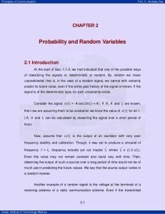
It should be mentioned that the four-parameter Weibull probability distribution simplifies to a three-parameter Rayleigh distribution [12-14] with an appropriate parameter substitution   2 and   2 . The three parameters  ,  , and  do not have independent effects on the quantile distribution, Eq. (6), and their contributions can be modeled with two of the parameters. Here, without loss of generality, it is assumed that  is a known constant, e.g.   2 , and the other two parameters  and  are assumed to be unknown variables. The effect of parameters  ,  , and  on the quantile distribution of the fourparameter Weibull model is studied in Fig. 1. As shown in Fig. 1 (a), the increase in the parameter  elevates the quantile value of the same probability and causes a longer distribution tail. The effect of  is similar throughout the quantile distribution as it amplifies the linear term. Parameter  indicates the amplification of the quadratic term and has a sensible effect on the tail distribution while its contribution to the distribution of x n  1.0 is limited. The shape parameter  affects both linear and non-linear terms and essentially defines the distribution curvature. Regarding the distributions shown in Fig. 1 (b),   2.0 causes a longer distribution tail than that of the three-parameter Rayleigh distribution with   2.0 , while   2.0 has the opposite effect. As shown in

8

this figure, the distribution tail is highly sensitive to the value of the parameter  while the distribution of normal events, i.e. x n  2.0 , is not significantly affected by value of

 . It should be noted that  has a constant effect on the entire quantile distribution where positive and negative  shift the distribution up and down, respectively.

9

10

 = 1.0  = 1.2  = 1.4  = 1.6

(P)

8

x

n

6 4 2 0 0 10

0.1 0.05 10

0

-1

10

-2

10

-0.05

-3

10

-4

-0.1

 /

P=(1-u)

(a)

 = 1.50  = 1.75  = 2.00  = 2.25  = 2.50

10

x

n

(P)

15

5 0.1 0 0 10

0.05 10

0

-1

10

-2

10

-0.05

-3

10

-4

-0.1



P=(1-u)

(b)

 = 1.50  = 1.75  = 2.00  = 2.25  = 2.50

10

x

n

(P)

15

5 1.6 0 0 10

1.4 10

-1

10

1.2

-2

10

-3

10

-4

1



P=(1-u)

(c) Fig. 1. Effect of parameter values on the quantile distribution of four-parameter Weibull model: (a)   2.0 and (b)   1.0 , (c)   0.05 .

10

3. Model statistics and empirical parameter estimation The conventional method of moments (MoM) and the more recently developed method of L-moments (MoLM) are used to estimate the unknown parameters of the four-parameter Weibull distribution model, i.e.  ,  ,  , and  . In the following sections, the general characteristics of these two moment-based parameter estimation methods are briefly overviewed and their specific application to the four-parameter Weibull distribution model is discussed. 3.1.

Method of Moments

Ordinary moments are basic statistics commonly used to characterize random variables and also applied for empirical parameter estimation purposes. By definition, the central moments of a random variable X with quantile function of x  u  are obtained from

 1  X    x  u  du 1

n 1

0

 n  X     x  u    1  X   du 1

0

n

n 1

(11)

The mean  1  X  represents the centroid of the distribution and the variance

 X 2  2  X  is a measure of the distribution dispersion around its center. Other useful statistics are the dimensionless third and fourth moments respectively called skewness

s X   3  X   X 3 and coefficient of excess kurtosis K X   4  X   X 4  3 . Substituting the quantile function of four-parameter Weibull model, Eq. (6), in Eq. (11), the relation for the first four moments of the four-parameter Weibull distribution are

11



derived and presented in Eq. (12). In this equation   z    e  t t z 1dt indicates the 0

well-known gamma function. In the MoM, the estimates of the unknown model parameters are obtained by equating the distribution moments, Eq. (12), with their corresponding sample moments and solving the system of equations numerically. The unbiased estimates of the first four sample moments can be obtained from a sample data (see e.g. [19]).

12

 1  n    

2 2



2   

  1   , 

(12)

3 4  2 4  1 2  2    4  2             3  3      2 k   1             2 2   1 2   2   2 k    1    ,    

 2  n  

4  3 6  24 16 3   6  6     4    2    2  2          2 5 3    12 8 4  2  5   5      3     2    2  1     2      4    1           2 4 3   6 4 4 2  2  4   4      3    1    2   2    1      2           3 3   6 2 3   3   3      2    1    2  1    ,     

 3  n  

8 4 8  12 6 6 4  2   8    2   4     2      6     2    3   2           3 7 4    36 30 6 2  7  8    2   3     2      5     2      6    1         24 24    4     2    1    3   2    1     2    6 2  2 6  16 10 12 2 2  6  6      4     2      5    1    3   2    1         8 3 4 24    2    2   4    2 1    2   3     2    1     2     3 5 4    9 6 12 2  5  5    2   3    1      3     2      4    1         6 6   1    2  2    3   2    3 1     2    4 4   12 12 3 4  2  4   4      3    1    2   2    1    3   2    .      

 4  n  

13

3.2.

Method of Linear Moments

Hosking [15] introduced the L-moments as a linear function of the random variable quantile function multiplied by an orthogonal polynomial, specifically,

 n  X    x  u  Pn*1  u  du 1

(13)

0

where the shifted Legendre polynomial of degree n , Pn*  u  , is defined as r

Pn*  u    pn*, k u k

(14)

k 0

and

 1  n  k !  2  k !  n  k ! nk

p

* n ,k

(15)

By definition,  1 is the L-location or mean of the distribution,  2 is the L-scale, and   2 1 ,  3  3 2 , and  4  4 2 are L-Coefficient of variation, L-skewness, and L-kurtosis, respectively. The main difference between ordinary moments and Lmoments is that moments give greater weight to the extreme tails of the distribution. The weight given to the extreme tail, i.e. u  1 , increases by

 x u 

n

and by u n

respectively for ordinary moments, and L-moments. For most probability distributions

x  u  grows much faster than u as u  1 ; especially in the case of four-parameter Weibull model with   0 the distribution has no upper bound and therefore x  u    as u  1 .

14

The first four L-moments of the non-linear variable  n are derived by applying the quantile function of four-parameter Weibull model Eq. (6) in Eq. (13) , specifically

1   n    

2 2



 2  n  

2 2

 3  n  

2  2



2   

  1   , 

1  1 2    2     1  1 2   1   , 2

1  3 1 2 

1

 2 1 3



 2      1 1 1  3 1 2   2 1 3  1   ,  2



 4  n  

(16)

2



2  2

1  6 1 2 

 10 1 3

2

 5 1 4 



 2      1 1 1 1  6 1 2   10 1 3  5 1 4   1   .  2



2



As shown in Eq.s (12) and (16), the nth distribution moment is a polynomial of degree

n of the parameters  and  while L-moments are linear functions of these parameters. Both moments and L-moments are non-linear functions of the Weibull parameters



and  . For an ordered sample

x1:Ns  x2:Ns    xNs :Ns , the unbiased sample

estimates of the L-moments can be estimated from [19] n

ln 1  X    pn, k  n

n  0,1,..., N s  1

k 0

(17)

where the coefficients pn, k are introduced in Eq. (15), and  n is defined as

 n  Ns

1

 N s  1    n 

1

 j  1  x j:N s j  n 1  n  Ns



(18)

15

where the brackets denotes the binomial coefficients. It was shown in studies by Hosking [15, 19] that high order sample L-moments are considerably less biased than the corresponding sample moments especially for samples with limited number of observations. Similar to MoM, the parameter estimation with MoLM starts with defining the system of equations by equating the distribution L-moments, Eq. (16), with their corresponding sample estimators, Eq. (17). Next, the system of equations is solved numerically for the unknown model parameters.

4. Evaluation of Extreme Statistics Assuming that  n are independent identically distributed (i.i.d) random variables the PDF f max and CDF F max of the maxima  max in N observations can be obtained from the ordered statistics theory [20], specifically as

f max  x   N f n  x   F n  x   F max  x    F n  x  

N

N 1

(19)

where f n  x  and F n  x  are the PDF and CDF of non-linear random variable defined in Eq.s (6) and (7) respectively for the cases with   0 and   0 . This approach has been used to estimate the statistics of wave crest maxima utilizing the theoretical Rayleigh-Stokes crest distribution [21-24]. The assumption that consecutive wave crests are independent may not be theoretically well justified and the common positive correlation of successive wave crests may lead to conservative estimates of the crest

16

maxima from Eq. (19). However, the results of previous studies [23, 24] indicate that this approximation is reasonably accurate for number of waves N  100 . It can be shown that for large number of waves, the asymptotic form of the maxima distribution of the four-parameter Weibull model belongs to the Gumbel domain of attraction with CDF of

  x  aN F max  x   exp   exp   bN  

   

   x  

(20)

where aN and bN are the extreme parameters and their relations with the model parameters and the number of waves N are a N     2  ln  N  

2

bN   2  ln  N   1 

2

   ln  N  

1

  ln  N  

2

    ln  N   11    ln  N  1     

(21)

From this, the first three moments of  max are obtained as

 1  max   aN  bN  EM ,  2  max  

2

bN2 ,

6  3  max   2 R  3 bN3 .

(22)

where  EM  0.5772 is the Euler-Mascheroni constant and  R  z  is the Riemann zeta function which at z  3 has a value of approximately  R  3  1.2021 . Similarly, the first three L-moments of  max are derived as

1  max   aN  bN  EM ,  2  max   bN ln  2  ,  3  max   bN  2 ln  3  3ln  2   .

(23)

17

For illustrative purposes, the effect of four-parameter Weibull model parameters

 ,  , and  on the quantile distribution of maxima x

max

 P

is presented in Fig. 2.

Note that the Weibull model distribution with   0 has an upper bound, which is considered in the estimation of probability distributions in Fig. 2.

18

 =1.0

20

 =1.2  =1.4

15 10

x

 max

(P)

 =1.6

5 0.1 0 0 10

0.05 10

0

-1

10

-2

10

-0.05

-3

10

-4

-0.1

 /

P=(1-u)

(a)  = 1.50  = 1.75  = 2.00  = 2.25  = 2.50

20

10

x

 max

(P)

15

5 0.1 0 0 10

0.05 10

0

-1

10

-2

10

-0.05

-3

10

-4

-0.1



P=(1-u)

(b)  = 1.50  = 1.75

20

 = 2.00  = 2.25  = 2.50

10

x

 max

(P)

15

5 1.6 0 0 10

1.4 10

-1

10

1.2

-2

10

-3

10

-4

1



P=(1-u)

(c) Fig. 2. Effect of parameter values on the quantile distribution of maxima: (a)   2.0 and (b)   1.0 , (c)   0.05 .

19

5. Model application and evaluation 5.1.

Model test data

The data sets to be analyzed in this study were obtained in a model test investigating the response behavior of a 1:40 scale model of a deepwater unmanned mini-TLP platform subject to random seas. Selected particulars of the mini-TLP model are presented in Table 1 and additional model test details can be found in the open literature [16, 17]. Each individual recorded time series represented a 3-hr design sea at prototype scale. The design seas were modeled using a JONSWAP wave spectrum with a significant wave height of 13.1m , a peak period of 14.0s , and a spectral peakedness factor of 2.2 . This design sea represented a 100-year Gulf of Mexico storm condition. The experimental study was conducted for both compliant and fixed hull configurations, but only the measurements obtained for the fixed hull quartering sea configuration are used in this study. This hull orientation along with the location of the air-gap probe A3 and wave run-up probes R1 and R2 is shown in Fig. 3 Table 1 Main particulars of the prototype mini-TLP.

Draft Column Diameter Column Spacing Pontoon Height Pontoon Width Water Depth

28.50 m 8.75 m 28.50 m 6.25 m 6.25 m 668 m

20

N R1

E

R2 A3

Fig. 3. Plan view of the mini-TLP model test and the wave probe locations.

5.2.

Estimating Model Bias, Variance and Error

The models performance is evaluated utilizing the semi-parametric bootstrap simulation. Bootstrap analysis is typically used to determine the bias, variance, and rootmean-squared error (RMSE) associated with a sample estimate ˆ of a parameter of interest  [25, 26], specifically

  M

 ˆ 

ˆ 

1 M

 2ˆ 

2 1 M *   i*    M  1 i 1

i 1

* i

RMSE ˆ   ˆ 2   ˆ2

(24)

(25)

(26)

21

where i* is the estimate of  from ith bootstrap sample, M is the number of bootstrap samples, and ˆ and  2ˆ are the bootstrap estimates of the true bias and true variance. In the semi-parametric bootstrap method, the independent samples of equal size to the original sample are generated with replacement from a smoothed empirical distribution with a parametric tail distribution. For this purpose, Kernel density estimation [27] is utilized to estimate the major part of the probability distribution and the distribution tail is modified with Generalized-Pareto distribution. The semi-parametric bootstrap is more suited for extreme analysis as compared to the conventional bootstrap analysis. Additional details about the semi-parametric bootstrap analysis can be found in [28]. In Table 2, the estimates of the model parameters of four-parameter Weibull (4Par. Weibull) three-parameter Rayleigh (3-Par. Rayleigh) models calculated for the three samples measured at R1, R2, and A3 are compared (see Fig. 3 for the probes location). For a more complete comparison, the estimates of both MoLM and MoM are presented in this table. Note that the parameters here are estimated from one 3-hr realization with approximately N s  1, 000 observations. The samples are normalized with respect to the first-order standard deviation of the incident wave surface elevation   estimated from its relation with significant wave height   H s 4  3.28m . As shown in Table 2, the parameter estimates of MoLM and MoM of the same model are reasonably close. The estimates of linear contribution  of four-parameter Weibull and three-parameter Rayleigh models are in an acceptable agreement and the values are significantly larger than 1.0. The largest value of parameter  is estimated for wave run-up at R2 that is an

22

indication of the relatively large contribution of diffracted waves at this location. The four-parameter Weibull model consistently has estimated a larger absolute  . As shown in Fig 1. (b), the negative  balances the large first-order contribution on the tail distribution. More interestingly, the four-parameter Weibull shape parameter  has a value smaller than that of the three-parameter Rayleigh model with   2.0 . This, as indicated in Fig 1. (c), decreases the distribution curvature of the four-parameter Weibull as compared to that of the three-parameter Rayleigh distribution. The shifting parameter

 is consistently negative in the studied cases which shifts the model distributions downward and causes non-zero probability for x n  0 . Since negative wave crests and run-ups are not physically meaningful, the distributions are only defined for x n  0 and





it is assumed that Prob  x  0  = Prob x n  0 .

23

Table 2. Parameter estimates of four-parameter Weibull and three-parameter Rayleigh distribution models

Parameter

ˆ

ˆ

ˆ

ˆ

Model 3-Par. Rayleigh 3-Par. Rayleigh 4-Par. Weibull 4-Par. Weibull 3-Par. Rayleigh 3-Par. Rayleigh 4-Par. Weibull 4-Par. Weibull 3-Par. Rayleigh 3-Par. Rayleigh 4-Par. Weibull 4-Par. Weibull 3-Par. Rayleigh 3-Par. Rayleigh 4-Par. Weibull 4-Par. Weibull

Parameter Crests Estimation @ A3 MoLM MoM MoLM MoM MoLM MoM MoLM MoM MoLM MoM MoLM MoM MoLM MoM MoLM MoM

1.747 1.759 1.728 1.723 -0.093 -0.100 -0.136 -0.127 2.000 2.000 1.735 1.772 -0.399 -0.402 -0.248 -0.280

Run-up @ R1

Run-up @ R2

1.907 2.169 1.915 1.919 0.046 -0.055 -0.161 -0.163 2.000 2.000 1.469 1.446 -0.504 -0.631 -0.105 -0.090

1.598 1.632 1.627 1.616 -0.006 -0.020 -0.108 -0.091 2.000 2.000 1.612 1.673 -0.429 -0.443 -0.234 -0.280

In Fig.s 4, 5, and 6, the quantile distributions and the quantile RMSE distributions of the wave samples measured at R1, R2, and A3 are shown, respectively. The sample distributions in these figures are obtained from the semi-parametric approach and also applied in the bootstrap analysis. The 95% confidence intervals (CI), as well as the RMSE distributions are obtained from utilization of 20,000 bootstrap samples. As shown in Fig. 4 (a), the sample distribution at R1 starts with an extremely steep slope which follows with a relatively mild slope for x n  4.8 . The slope change in the tail part of the distribution is common in wave measurements of extreme

24

environments and is mainly caused by an energy loss mechanism, e.g. wave breaking. It is observed that the three-parameter Rayleigh model is mostly affected by the initial steep slope and successfully captures the distribution of x n  4.8 , while overestimates the larger wave run-ups. The four-parameter Weibull model is successful in capturing the sample tail distribution while slightly deviates from the sample distribution in the range of 3.5  x n  4.9 . Regarding the RMSE distributions in Fig. 4 (b), the fourparameter Weibull and three-parameter Rayleigh models perform similarly for x n  3 . The three-parameter Rayleigh model found to be more accurate for 3.0  x n  4.8 , while four-parameter Weibull model performs better in capturing the probability distribution of x n  4.8 . The local peak in the RMSE distributions around P  0.1 is due to the slope change in the sample tail distribution. Wave run-up measurements at R2 are less energetic and less non-linear than those at R1 resulting in a probability distribution with a milder initial slope and less significant slope change of the tail distribution. As shown in Fig. 5 (a), the distribution estimates of MoM and MoLM converge reasonably well and both three-parameter Rayleigh and four-parameter Weibull models are successful in capturing the probability distribution of data. It is also observed that three-parameter Rayleigh model slightly overestimates the extreme wave run-ups of x n  4.2 , while four-parameter Weibull model, especially the distribution estimated by MoM, accurately represents the sample tail distribution. The error distributions in Fig. 5 (b) clearly indicate an agreement between the model estimates as well as an acceptable accuracy of four-parameter

25

Weibull and three-parameter Rayleigh models in capturing the sample distribution. Regarding the results shown in Fig. 6, both four-parameter Weibull and three-parameter Rayleigh model are considerably successful in capturing the sample probability distribution of wave crests at A3 as the sample distribution does not show any irregularity. Table 3 shows the estimates of expected maximum elevation ˆ1  max  in

N  1000 waves obtained from application of the estimated model parameters, given in Table 2, into Eq.s (21) and (22). Additionally, the estimates of ˆ1  max  obtained from the sample distribution and empirical Rayleigh and empirical Weibull distributions are provided in this table. Note that the values in this table are normalized with respect to the incident wave standard deviation   3.28m . As expected, the wave run-up sample at R1 has the highest ˆ1  max  and the next largest ˆ1  max  is predicted for wave run-up sample at R2. For the studied examples, the estimates of MoLM and MoM of the same model are reasonably close. The results shown in Table 3 clearly indicate that the empirical Weibull distribution significantly overestimates the extreme values. The empirical Rayleigh distribution estimated more representative extreme values than the empirical Weibull distribution, even though the total sample distribution is more accurately captured by Weibull distribution. In the studied examples, the three-parameter Rayleigh model consistently predicts larger expected maximum than both the fourparameter Weibull model and the sample distribution. The issue is more sensible in the case of wave run-ups at R1 for which the three-parameter Rayleigh model has predicted

26

an unrealistically large expected maxima of about 7.50 (equivalent to 24.6m). The overestimation is mainly due to inability of three-parameter Rayleigh model in capturing the negative slope change in the tail distribution. This shortage is improved in the fourparameter Weibull model with utilization of the fourth moment and as shown in Table 3, the estimates of four-parameter Weibull model follows the sample estimates reasonably well.

27

8 7 6

x n ( P )

5 4 3

Sample-Dist. 3-Par Rayleigh, MoLM

2

3-Par Rayleigh, MoM 4-Par Weibull, MoLM

1

4-Par Weibull, MoM 95% CI

0 0 10

-1

-2

10

10

-3

10

-4

10

P=( 1 -u )

(a) 0.8

RMSE ( x  n ( P ) )

3-Par Rayleigh, MoLM

0.7

3-Par Rayleigh, MoM 4-Par Weibull, MoLM

0.6

4-Par Weibull, MoM

0.5 0.4 0.3 0.2 0.1 0 0 10

-1

-2

10

10

-3

10

-4

10

P=( 1-u)

(b) Fig. 4. Wave run-up at R1: (a) quantile distributions, (b) RMSE distributions.

28

8 7 6

n (P )

5 4 3

Sample-Dist. 3-Par Rayleigh, MoLM

2

3-Par Rayleigh, MoM 4-Par Weibull, MoLM

1

4-Par Weibull, MoM 95% CI

0 0 10

-1

-2

10

10

10

-3

10

-4

P=( 1 -u )

(a) 0.8

RMSE ( x  n ( P ) )

3-Par Rayleigh, MoLM

0.7

3-Par Rayleigh, MoM 4-Par Weibull, MoLM

0.6

4-Par Weibull, MoM

0.5 0.4 0.3 0.2 0.1 0 0 10

10

-1

10

-2

10

-3

10

-4

P=( 1 -u )

(b) Fig. 5. Wave run-up at R2: (a) quantile distributions, (b) RMSE distributions.

29

8 7 6

n (P )

5 4 3

Sample-Dist. 3-Par Rayleigh, MoLM

2

3-Par Rayleigh, MoM 4-Par Weibull, MoLM

1

4-Par Weibull, MoM 95% CI

0 0 10

-1

-2

10

10

10

-3

10

-4

P=( 1 -u )

(a) 0.8

RMSE (  n ( P ) )

3-Par Rayleigh, MoLM

0.7

3-Par Rayleigh, MoM 4-Par Weibull, MoLM

0.6

4-Par Weibull, MoM

0.5 0.4 0.3 0.2 0.1 0 0 10

10

-1

10

-2

10

-3

10

-4

P=( 1 -u )

(b) Fig. 6. Wave crests at A3: (a) quantile distributions, (b) RMSE distributions.

30

Table 3. Estimates of expected maximum elevation in 1000 waves.

Model Sample Distribution Empirical Rayleigh Empirical Weibull 3-Par. Rayleigh-MoLM 3-Par. Rayleigh -MoM 4-Par. Weibull -MoLM 4-Par. Weibull -MoM

Crests at A3 4.82 5.10 6.38 4.96 4.91 4.77 4.83

Run-ups at R1 5.64 6.48 8.94 7.56 6.93 5.56 5.54

Run-up at R2 5.39 5.10 7.17 5.66 5.57 5.16 5.31

6. Conclusions The four-parameter Weibull probability distribution was introduced as an improvement to the three-parameter Rayleigh distribution of weakly non-linear variables. The four-parameter Weibull probability distribution was introduced as an improvement to the three-parameter Rayleigh distribution of weakly non-linear variables. In development of both models, the theoretical information of the variable was based to derive the mode structure using the quadratic transformation of the linear random variable. The empirical estimates of the model parameters were obtained from method of linear moments, which improved the flexibility of the models in capturing the probability distribution of sample data. These empirical probability distribution models can be used for probability distribution estimation of a wide range of non-linear random variables in different fields of engineering. The four-parameter Weibull formulation takes advantage of an unknown shape parameter that was assumed to be a fixed constant in the three-parameter Rayleigh distribution. The additional parameter improves the flexibility of the four-parameter

31

Weibull probability distribution in estimating the sample tail distribution. The fourparameter Weibull model was utilized to evaluate the extreme statistics and deriving the asymptotic probability distribution of maxima in large number of observations. The estimates of four-parameter Weibull model parameters were obtained from application of conventional method of moments and the method of linear moments. For this purpose, the first four distribution moments were derived in terms of the model parameters and consequently the relations were used to evaluate the parameters. For illustrative purposes, the four-parameter Weibull probability distribution was applied to estimate the probability distribution of wave run-up measurements over a vertical column of a TLP model test and the probability distribution of wave crests measured at the center of the platform inside the moon-pool area. The root-meansquared error of the quantile distributions estimated from application of the bootstrap analysis was utilized as the measure to evaluate the models performance. In the cases studied, the model parameters estimated by conventional method of moments and method of L-moments are in a reasonable agreement. The three-parameter Rayleigh and the four-parameter Weibull models perform similarly for the major part of the distribution while the difference between the model estimates is more sensible on the distribution tail. It was verified that four-parameter Weibull model is more flexible than three-parameter Rayleigh model in estimating the sample tail distribution. The studied wave run-up samples indicated a sudden negative slope change in the distribution tail which was not completely captured by three-parameter Rayleigh model. This caused an overestimation in the extremal predictions of the three-parameter Rayleigh model. The

32

four-parameter Weibull found to be more robust in capturing the slope change of the tail distribution and the model predicted more reliable extreme statistics.

Acknowledgements

The authors would like to gratefully acknowledge the partial financial support of the Texas Engineering Experiment Station and the Wofford Cain’13 Chair endowment during this research investigation. In addition, we would like to recognize Dr. Per S. Teigen of Statoil Norway and the Offshore Technology Research Center for permission to utilize the experimental data presented in this study.

References [1]

M.A. Tayfun, Distribution of large wave heights, Journal of Waterway, Port, Coastal, and Ocean Engineering 116 (1990) 686-707.

[2]

M.S. Longuet-Higgins, On the statistical distribution of the heights of sea waves, Journal of Marine Research 11 (1952) 245-66.

[3]

D.E. Cartwright, M.S. Longuet-Higgins, The statistical distribution of the maxima of a random function, Proceedings of the Royal Society of London-Series A: Mathematical and Physical Sciences 237 (1956) 212-32.

[4]

R.G. Dean, R.A. Dalrymple, Water Wave Mechanics for Engineers and Scientists, Advanced Series on Ocean Engineering-Volume 2, World Scientific, 2007.

[5]

M. Arhan, R.O. Plaisted, Non-Linear deformation of sea wave profiles in intermediate and shallow water, Oceanologica Acta 4 (1981) 107-15.

[6]

C.C. Tung, N.E. Huang, Peak and trough distribution of nonlinear waves, Journal of Ocean Engineering 12 (1985) 201-9.

[7]

D.L. Kriebel, T.H. Dawson, Nonlinearity in wave crests statistics, In: Proc. 2nd international symposium on ocean wave measurement and analysis (1993) 61-75.

[8]

D.L. Kriebel, T.H. Dawson, Nonlinear effects on wave groups in random seas. Journal of Offshore Mechanics and Arctic Engineering 113 (1991) 142-7.

33

[9]

F. Fedele, F. Arena, Weakly nonlinear statistics of high random waves, Journal of Physics of Fluids 17 (2005) 1-10.

[10] M.A. Tayfun, Statistics of nonlinear wave crests and groups, Journal of Ocean Engineering 33 (2006) 1589-1622. [11] D.L. Kriebel, Non-linear run-up of random waves on a large cylinder, In: Proc. 12th international conference of ocean, offshore and arctic engineering (1993) 4955. [12] A.H. Izadparast, J.M. Niedzwecki, Estimating wave crest distributions using the method of L-moments, Journal of Applied Ocean Research 31 (2009) 37-43. [13] A.H. Izadparast, J.M. Niedzwecki, Probability distributions for wave run-up on offshore platform columns, In: Proc. 28th international conference of ocean, offshore and arctic engineering (2009) 607-15. [14] A.H. Izadparast, J.M. Niedzwecki, Probability distributions of wave run-up on a TLP model, Journal of Marine Structures 23 (2010) 164-86. [15] J.R.M. Hosking, L-moments: Analysis and estimation of distributions using linear combinations, Journal of the Royal Statistical Society-Series B: Methodological 52 (1990) 105-24. [16] P.S. Teigen, J.M. Niedzwecki, S.R. Winterstein, Wave interaction effects for noncompliant TLP, In: Proc. 11th international offshore and polar engineering conference (2001) 453-61. [17] J.M. Niedzwecki, P-YJ. Liagre, J.M. Roesset, M.H. Kim, P.S. Teigen, An experimental research study of a Mini-TLP, In: Proc. 11th international offshore and polar engineering conference (2001) 631-4. [18] P.Z. Peebles, Probability, random variables, and random signal principles, McGraw Hill, 2001. [19] J.R.M. Hosking, J.R. Wallis, Regional frequency analysis an approach based on Lmoments, Cambridge University Press, 1997. [20] M.R. Leadbetter, G. Lindgren, H Rootzen, Extremes and related properties of random sequences and processes, Springer Series in Statistics, Springer-Verlag, 1983. [21] R. Nerzic, M.A. Prevosto, Quadratic-Weibull model for the distribution of maximum wave and crest heights, In: Proc. 7th international offshore and polar engineering conference 1997 (367-77).

34

[22] T.H. Dawson, Maximum wave crests in heavy seas, Journal of Offshore Mechanics and Arctic Engineering 122 (2000) 222-4. [23] M. Prevosto, H.E. Krogstad, A. Robin, Probability distributions for maximum wave and crest heights, Journal of Coastal Engineering 40 (2000) 329-60. [24] H.E. Krogstad, S.F. Barstow, Analysis and applications of second-order models for maximum crest height, Journal of Offshore Mechanics and Arctic Engineering 126 (2004) 66-71. [25] B. Efron, Bootstrap methods: Another look at the jackknife, The Annals of Statistics 7 (1979) 1-26. [26] B. Efron, R. Tibshirani, An introduction to the bootstrap, Chapman & Hall/CRC, 1993. [27] B.W. Silverman, Density estimation for statistics and data analysis, Monographs on Statistics and Applied Probability, Chapman and Hall, 1986. [28] J. Caers, M.A. Maes, Identifying tails, bounds and end-points of random variables, Journal of Structural Safety 20 (1998) 1-23.