FOREIGN DIRECT INVESTMENT VERSUS JOINT VENTURES

By

YUTING LI

B.A., Huazhong University of Science and Technology, 2009

A THESIS

submitted in partial fulfillment of the requirements for the degree

MASTER OF ARTS

Department of Economics College of Arts and Sciences

KANSAS STATE UNIVERSITY Manhattan, Kansas

2011 Approved by: Major Professor Yang-Ming Chang

Copyright YUTING LI

2011

All rights reserved. No part of this document may be reproduced or transmitted in any form or by any means, electronic, mechanical, photocopying, recording, or otherwise, without prior written permission of the author.

Abstract This paper studies economic factors that affect a multinational’s decision between serving a foreign market via foreign direct investment (FDI) and setting up a joint venture (JV) with a local firm in the host country. The factors that we consider include the substitutability of products produced by competing firms, as well as the hotly debated intellectual property rights (IPRs) protection. In a simple North-South framework, we show that JV is the equilibrium market structure when the degree of R&D spillover is moderate, products are considerably substitutable, and IPRs strong. The government of South needs to maintain a minimum level of IRP to encourage an effective JV. For increasing social welfare, the South also needs to have a policy that limits foreign ownership in a JV.

Table of Contents List of Figures ................................................................................................................................. v Chapter 1 -Introduction ................................................................................................................... 1 Chapter 2 - The Model .................................................................................................................... 4 Basic assumptions ....................................................................................................................... 4 Chapter 3 - Output competition stage ............................................................................................. 7 Green field FDI case ................................................................................................................... 7 JV case ........................................................................................................................................ 9 Chapter 4 - The equilibrium choice of an entry mode .................................................................. 11 Chapter 5 - Bargaining in a joint venture...................................................................................... 16 Chapter 6 - Welfare of the South .................................................................................................. 18 Chapter 7 - Concluding remarks ................................................................................................... 22 References Or Bibliography ......................................................................................................... 24 Appendix A .................................................................................................................................. 26

iv

List of Figures Figure 2.1 First Figure in Chapter 2............................................................................................... 5 Figure 4.1 First Figure in Chapter 4............................................................................................. 13 Figure 4.2 Second Figure in Chapter 4 ........................................................................................ 14 Figure 4.3 Third Figure in Chapter 4 ........................................................................................... 15 Figure 6.1 First Figure in Chapter 6............................................................................................. 21 Figure 6.2 Second Figure in Chapter 6 ........................................................................................ 21 Figure A.1 First Figure in Appendix A......................................................................................... 27

v

1. Introduction The alliance of IBM and Lenovo made Lenovo the world’s third largest PC maker. Recently Lenovo formed a PC joint venture with Japanese PC maker NEC. As part of the deal, the companies said in a statement that they will establish a new company called Lenovo NEC Holdings B.V. to be registered in the Netherlands. NEC will receive $175 million from Lenovo through the issuance of Lenovo's shares. Lenovo, through a unit, will own a 51% stake in the joint venture, while NEC will hold a 49% stake. Our model seeks to theoretically analyze similar scenarios of the relationship between foreign direct investment, joint venture, and foreign ownership. With the development of international trade and globalization, firms are no longer limited to domestic production or domestic sales. There are several possible ways for multinational enterprises to enter a foreign market. The existing literature has mainly considered three different modes of serving a host country market. They are licensing, export, and foreign direct investment (FDI). A great deal of research has discussed licensing in details. For example, Mukherjee (2007) examines different forms of licensing contracts. One objective is to explain these different possibilities as the results of the trade-off between incentives of saving transportation cost of exporting and reducing competition after licensing. Mukherjee (2010) further discusses the implications of both fixed-fee licensing and royalty licensing on the competition and welfare of host counties under Bertrand and Cournot competition. Following Ethier and Markusen (1996), Saggi (1999) and Kabiraj and Marjit (2003), Sinha (2009) shows that a foreign firm can strategically choose licensing prior to its choice of an entry mode between export and FDI, which might result in a welfare loss for the host country depending on the structure of license fee. The 1

paper suggests the host country to utilize an optimal tariff scheme or a ban on licensing to maximize its social welfare. Two forms of foreign direct investments that directly involve the transfer of resources (such as capital, technology, and personnel) are FDI and JV. That is why many developing countries compete to attract FDI and encourage their firms to set up JVs with foreign firms, hoping to bring in advanced technology. The multinational enterprise (MNE) can build a sole ownership company (i.e., FDI) in the host country through the acquisition of an existing entity or the establishment of a new enterprise. Direct ownership provides a high degree of control in the operations but it requires a high level of resources and a high degree of commitment. An alternative strategy is to build a Joint Venture (JV) with a local firm. Possible benefits of forming a JV include political connections, existing facilities, and an efficient distribution channel. Sometimes the foreign firms have to build a JV in order to enter the local market when FDI is not allowed by local regulations. However, this partial ownership of JV cuts the degree of control over technology and intangible assets from the MNE. Thus, JV is commonly believed to have a higher possibility of technology spillovers. For example, Dimelis and Louri (2002) find that technology spillovers are stronger when foreign firms are in minority positions. Some empirical studies including Aitken and Harrison (1999), Liu (2002) and Javorcik (2004) provide supporting evidence for this view. It appears that relatively little research has been done to analyze the role of joint ventures in serving a foreign market. Muller and Schnitzer (2003) study JVs and technology transfer but the setting is much different from the present study. The authors discuss a game between a multinational enterprise and the host-country government under different policy structures and show how policy could be designed to make technology transfer profitable for both even with 2

high spillovers. Leahy and Naghavi (2010) consider their study on FDI versus JVs to be the first theoretical work that investigates intellectual property rights (IPRs) issues surrounding JVs. The authors use a simple Cournot Competition model similar to the model developed by Chin (1990). The analytical framework of Chin (1990) has been widely employed to discussing IPR and technology transfer problems such as Naghavi (2007). Leahy and Naghavi (2010) find that JV is the equilibrium market structure when R&D intensity is moderate and IPRs strong. They also concluded that policies to limit foreign ownership in a JV can increase the welfare of the host countries. This conclusion is based on the assumption that the share of foreign ownership is exogenously given. In this paper, we attempt to endogenize the share of foreign ownership by applying a sharing rule widely used in the rent-seeking literature. We find that the equilibrium foreign ownership should be more than fifty percent. Further, our model differs from Leahy and Naghavi (2010) as we adopt a framework of product differentiation similar to the one in Ishikawa, Sugita, and Zhao (2009). We find a range of product differentiation within which JVs could take place. Moreover, our analysis allow for the possibility that there is partial transfer of technology from the foreign firm to the JV. We also analyze conditions under which full technology transfer is optimal for the foreign firm. The remainder of this paper is structured as follows. Section 2 presents the basic assumptions and structure of a simple North-South framework of imperfect competition to analyze issues on FDI and a JV. Section 3 examines the production decisions of all firms and the R&D decision of the MNE under an entry mode. Section 4 discusses the equilibrium mode of entry regarding the values of each related parameter. Section 5 analyzes the share of profits between the Northern and the Southern inside partners, as well as the optimal degree of 3

technology transfer. In Section 6, we examine the impacts of FDI and JV on the host country’s consumer surplus and social welfare. Concluding remarks can be found in Section 7.

2. The Model Basic Assumptions There are two local firms (denoted as S1 and S2) in the South and one foreign firm (denoted as F) from the North with superior technology. The Northern foreign firm attempts to enter the market in the South. Policies of the Southern government have been set before the Northern foreign firm entering the local market. We pay attention to interaction of the three firms in this Southern market. The foreign firm has to decide its mode of entry as either FDI or JV. We allow the Northern foreign firm and the Southern local firms to have differentiated products, so their products are not perfectly substitutable. There are good reasons for the Northern firm to form a joint venture with one of the Southern local firms such as to utilize the existing facilities and avoid fixed or set-up costs. A local firm may be willing to do so because the foreign firm posses a superior technology and the alliance can effectively reduce cost and competition. On the other hand, sharing of ownership in a JV will expose the foreign firm to higher risks of technology spillover if the IPRs are loose in the host country. This might be due to the fact that it is difficult to write a contract specifying exactly the right to use the intangible assets or technology and the mobility of skilled workers. The ownership structure is partially important when the multinational’s competitive advantage stems from intangible assets or technology leadership that can be costly to generate and easily imitate. Facing these trade-offs, the foreign firm may either enter the market by FDI or form a 4

joint venture (JV) with one of the Southern local firms by random match. If the JV takes place there will be two firms competing in the market. We will discuss a two-stage game here. At stage 0, the Southern government sets up its rules and regulations before the Northern firm enters the local market. In the first stage, the foreign firm chooses its mode of entry, the amount of technology transfer and the amount of cost-reducing R&D investment on technology. In the second stage, the firms compete in the product markets. We allow for product differentiation in the analysis. The sequences of the game are summarized in Figure 2.1. IPR & foreign ownership policy

FDI

JV

R&D investment

Production decisions

R&D investment & technology transfer

Production decisions

Figure 2.1 Sequence of the game

For analytical simplicity, the (inverse) market demands facing the Northern foreign firm and the Southern local firms are taken to be:

PF  aF  qF  r (q1  q2 )

(1a)

and 5

PL  aL  rqF  (q1  q2 ),

(1b)

where qF is the quantity of output produced by the foreign firm, q1 and q2 are respectively those of the local firms in the South with Q  q1  q2 . The parameter r (0  r  1) indicates the degree of substitutability between the foreign product and those of the local firms (with r = 0 and r = 1 reflecting no and complete substitutability, respectively). The parameters a F and a L represent market sizes. Product differentiation can be justified on the grounds that the foreign firm uses superior technology, which potentially leads to products that meet consumer demands better than local ones (Ishikawa, Sugita and Zhao, 2009).1 In the present model, only the foreign firm that has superior technology will make R&D investments. The Southern firms make no R&D investment. The South might lack the resources for R&D or the Southern firms may find it unprofitable to do so as it takes time for R&D to be turned into productivity. 2 The Northern firm’s R&D aimed at inventing more efficient production technologies and hence takes a cost-reducing form. The unit cost functions for the foreign firm and the local firms are given, respectively, as

C F    gx and C L   ,

(2)

where  ( ai ) is the pre-innovative basic unit cost, i  F , L (noting that parameter ai represents the size of market as shown in the demand function in (1)), x(  2 / g ) is the amount of cost-

1

For instance, when we talk about cell phones these days, everybody would want an iphone. The price of a 3G

iphone is almost double as a 3G phone from say Nokia with similar functions. Even though a 3G Nokia phone may be as good as an iphone in terms of all the functions a phone could have, consumers are willing to pay a couple more hundred dollars for the iphone because Apple fans recognize them as different. 2

Small or median size firms may not even exist for a long period of time.

6

reducing R&D investment by the foreign firm, and g indicates the effectiveness of the R&D process. In the case of a JV, we have to consider the situations that involve technology spillovers. Define  = bι , which captures the level of technology spillovers. The parameter  is itself a product of the absorptive capacity 0 ≤ b ≤ 1 (with b = 0 and b = 1 reflecting infinite and no absorptive capacity, respectively) and a measure of the weakness of IPR protection in the South 0 ≤ ι ≤ 1 (with ι = 0 and ι = 1 reflecting full and no protection, respectively), and determines the degree of spillovers.

3. Output Competition Stage Green field FDI case When the Northern foreign firm chooses to enter the local market through FDI, it competes with two Southern firms in the host country. It is usually assumed that fixed costs associated with FDI can be avoided or reduced by forming a JV to utilize already existing facilities of a local firm. Fixed costs of FDI are, however, left out of the model for simplicity. Adding fixed costs in the model will make JV more profitable and provide more incentives for the MNE to choose JV. In the case of FDI, the profits of the three firms are:

 F  [aF  qF  r (q1  q2 )  (  gx )]qF  x

(3a)

and

 Lj  [aL  rqF  (q1  q2 )   ]qLj ,

(3b)

where subscript F represents that the foreign firm engages in FDI, and Lj denotes its rival local firms with j  1, 2. For simplicity, we let a F    a L    A for the rest of the analysis. In the 7

final stage of the game, firms compete in the product markets in a Cournot manner and choose their optimal output taking the levels of outputs by other firms as given. Solving for the equilibrium outputs for the firms yields

qF 

(3 A  2rA  3 gx ) , 2(3  r 2 )

(4a)

qLj 

(2 A  rA  r gx ) . 2(3  r 2 )

(4b)

At the R&D investment stage, we assume that the foreign firm correctly foresees the equilibrium outcomes for product-market competition. We seek a solution that satisfies the subgame perfect Nash equilibrium. Fully informed of these outcomes, the Northern firm in the R&D stage chooses x to maximize its total profits:

(3 A  2rA  3 gx )2 F  x. 4(3  r 2 )2

(5)

Substituting the equilibrium outputs derived in equation (4) into the profit function of the Northern firm in (5) and taking the differentiation of the latter with respect to x, we derive the optimal level of R&D investment: x* 

A2 g (9  6r )2 . [4(3  r 2 )2  9 g ]2

(6)

It is instructive to examine the relationship between x* and r. Taking the derivative of x* with respect to r yields 2 2 2 x*  108 A g  3  2r  [3g  4(3  r ) (r  1) ] r [4(3  r 2 )2  9 g ]3

which implies that

x*  0 for g   4 (3  r 2 )(r  1)2 . 3 r 8

* It follows from the above analysis that for g  g  , we have x  0. This indicates that the r

higher the value consumers placed on the foreign product produced by a better technology (i.e., * r is closer to 0) the higher the level of R&D investment undertaken by the foreign firm (i.e., x

is higher). It can also be seen that the more effectiveness the cost-reducing R&D (i.e., g ) the * higher the level of R&D investment by the foreign firm. That is, x  0. This result is similar g

to that in Leahy and Naghavi (2010). Substituting x* in equation (6) into the profit functions of the firms, we have their optimal profits as follows:

F 

A2 (2r  3) 2 , 4(3  r 2 )2  9 g

(7)

 Lj 

A2 (12  2r 3  4r 2  6r  3g )2 . [4(3  r 2 )2  9 g ]2

(8)

We assume g  (12  2r 3  4r 2  6r ) / 3 to ensure that all firms produce nonnegative outputs and earn nonnegative profits. It comes as not a surprise that there is a positive association between the foreign firm’s profits and the effectiveness of its R&D. Interestingly, a very high value of g will drive the Southern firm out of the market, but this special case is not our focus here.

JV case Now we look at the situation when the foreign firm forms a JV with a local firm to serve the local market. We allow the foreign firm to partially transfer its superior technology, the level 9

of which is denoted as 0    1 (with  =0 and  =1 reflecting zero and full technology transfer respectively). This could be true as it might not always be in the best interest of the foreign firm to transfer its superior technology one hundred percent to a JV in real economy investment environment. We can think of several reasons for this, the foreign firm can face regulations of ownership from the local government which stop it from the gain of fully technology transfer. We assume a JV maximizes joint profits whoever firm holds the decision power and a fixed share of profits go to each partner. The profits of the firms under JV are

 J  [a  (qJ  rqo )   (  gx )   (1   )]qJ  x  [ A  (qJ  rqo )   gx ]qJ  x

(9a)

 o  [a  (rqJ  qo )   (  gx )   (1   )]  ( A  (rqJ  qo )   gx )qo ,

(9b)

and

where A  a   , subscript J representing a JV and O representing the Southern outside firm. We solve for the optimal levels of outputs produced by the JV firm and the outside firm as follows: qJ 

1 (2 A  2 gx  Ar  r  gx ) 4  r2

(10a)

qo 

1 (2 A  Ar  r gx  2 gx ). 4  r2

(10b)

and

We also solve for the optimal level of R&D investment undertaken by the JV firm as x* 

(r  2)2 A2 g 2 (r   2)2 [(r  2)2 (r  2)2  g 2 (r   2)2 ]2

It follows from equation (11) that we have the following comparative static derivatives: 2 2 2 2 2 2 2 x  2 A g (r   2) (r  2) [ g (r   2)  (r  2) (r  2) ]  0;  [(r  2)2 (r  2)2  g 2 (r   2)2 ]3

10

(11)

2 2 2 2 2 2 2 x  2 A gr (r   2) (r  2) [ g (r   2)  (r  2) (r  2) ]  0.  [(r  2)2 (r  2)2  g 2 (r   2)2 ]3

These results indicate that R&D investment is an increasing function of  , but is a decreasing function of  . Substituting x * into the profit functions of the firms, we have

J  o 

A2 (r  2)2 H

(12a)

A2 (r 3  2r 2  gr  2 2  gr  2  4r  2 g  2  2 g 2  8)2 , H

(12b)

where H  (16  8r 2  r 4  4 g 2  gr 2  2 2  4 gr  2 )  0 . The next step of the analysis is to analyze the entry mode decisions of the Northern firm by comparing the equilibrium profits as derived earlier. To do so, we analyze this issue in the next section.

4. The equilibrium choice of an entry mode Joint venture arises as the optimal choice when it can generate extra rent to be shared by the Northern firm and the Southern inside firm. If either the local inside firm or the MNE cannot get as much in JV as in FDI, they will have no incentive to form a JV. Therefore, a possibility frontier exists for the values of the parameters under which a JV is the equilibrium choice of the entry mode. That is, the JV firm’s overall profit should be no less than the sum of the foreign profit and the inside local firm’s profit in FDI. Such a boundary satisfies the following condition:

J  F I .

11

Substituting  J from equation (12a),  F from equation (7), and  I from equation (8) into the above condition yields

(r  2) 2 (2r  3) 2 (3g  2(r  2)(r 2  3)) 2   (r  2) 2 (r  2) 2  g 2 (r  2) 2 4(3  r 2 ) 2  9 g (4(3  r 2 ) 2  9 g ) 2

(14)

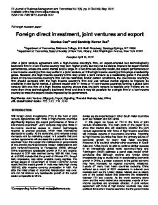
Keeping any pair of the four parameters constant, we can find the relationship of the other pair. Assuming the case of a full technology transfer (i.e.,   1 ) and 100 percent research effectiveness (i.e., g =1), we have from (14) that there is a combination of  and r within which JV is the equilibrium outcome. Figure 4.1 reflects the relationship in the above critical condition; regions underneath the lines are where a JV could be formed. As no curve exists for  > 0.5 and r < 0.5, Figure 4.1 illustrates for simplicity a case with a partial range of  and r .3

The analysis indicates that JV takes place only when the products of the MNE and the local firms are not substantially different. Intuitively, if the product of the MNE is so unique and the technology used is so exclusive, the MNE cannot take advantage of the existing facilities in the host country. Under these circumstances, the MNE will prefer to have complete ownership and decide to undertake FDI for the purpose of preventing technology spillovers when IRP protection is low and technology easy to copy. Even though the local firms would like to accept JV, the Northern firm will not offer it. When the products of the Northern and Southern firms are closer, the MNE can take advantages of the existing facilities while the South can enjoy the superior technology to reduce production costs. Both firms have incentives to join in the alliance. When we have 100% R&D and a full technology transfer, JV takes place only between firms whose products are at least 70% substitutable. If the IPR protection is stricter in the local market 3

To see this in full range, refer to Appendix A-1.

12

which makes JV more profitable, there will be more probabilities for firms producing differentiated goods when forming a JV( the range of r becomes larger).

ß

0.5

0.4

0.3

0.2

JV

0.1

0.0 0.5

0.6

0.7

0.8

0.9

1.0

r

Figure 4.1. A range of  and r that leads to a JV

The above analysis leads to PROPOSITION 1. Increasing the level of IPR protection in the South (that is, lowering the value of  ) reduces the losses due to imitation of the JV technology by the outsider firm and, consequently, increases the range of r over which a JV occurs. The relationship between  and  under JV when g =1, r =1 is shown in Figure 4.2. The figure illustrates that JVs are only offered and accepted when the degree of technology transfer is significantly high. If the IPR protection is stricter, JV becomes profitable even with less degree of technology transfer. The values of parameters should also satisfy the constraint

13

 FFDI   FJV   JV for the JV to be the equilibrium choice of the entry mode. We find that the minimum technology transfer rate is mim 0. 847 79 for  = 0, g = 1, r =1.

ß

0.5

0.4

0.3

0.2

JV

0.1

0.0 0.80

0.82

0.84

0.86

0.88

0.90

0.92

0.94

0.96

0.98

1.00

d

Figure 4.2. The relationship between  and  under JV

Based on the above analysis, we have PROPOSITION 2. Increasing the level of IPR protection in the South (that is, lowering the value of  ) reduces the losses resulting from technology spillovers, consequently, increases the range of  over which a JV occurs.

As the value of g decreases, the curve in Figure 4.1 and Figure 4.2 will move down and completely disappear when R&D effectiveness is smaller than a reasonable amount, see Appendix A-1 with graphs showing the full range of the two parameters. The higher research effectiveness, more room exists for JV to be formed. When r =1 and  =1, we get a graph for the relationship of  and g within which JV can take place similar to the result of Leahy (2010), shown as Figure 4.3. 14

ß

0.5

0.4

0.3

0.2

JV 0.1

0.0 0.0

0.1

0.2

0.3

0.4

0.5

0.6

0.7

0.8

0.9

1.0

1.1

1.2

1.3

1.4

1.5

g

Figure 4.3 The relationship of  and g that leads to a JV

From the above analysis, we have PROPOSITION 3. Increasing the level of the IPR protection in the South (that is, lowering the value of  ) increases the range of R&D efficiency (i.e. g ) over which a JV emerges as the market equilibrium. Leahy (2010) finds estimates for the absolute maximum value of  to be 0.348 that leads to JV. From the graphs presented in the present study, we find that the absolute maximum value of  consistent with a JV is no greater 0.4. This result is consistent with the findings of Leahy (2010). JV takes place only when the level of intellectual property rights protection is sufficiently high so that the insiders can exploit the advantages of merging. The proposition here is that raising the IPR protection in the South (lowering  ) reduces the potential losses due to spillover or imitation of the JV technology by the outsider firm. This increases the range of g over which a JV occurs.

15

5. Bargaining in a joint venture In this Section, we will determine the share of JV profits between the Northern firm and the Southern inside firm. Defining the share of the Northern firm as  (where 0 ≤  ≤ 1), the share of the Southern inside firm is 1-  . This is the departure of our analysis from earlier studies in the literature that focus on the extreme cases when  = 0 or 1 (e.g., Lin and Saggi, 2004; and Leahy and Naghavi, 2010). We assume the rule to decide the share is that the two parties will equally split the gain from form a JV. The two parties will receive exactly the same amount of extra net profit from JV compared to their profit under FDI. The gain that goes to each party within JV will be equal. Therefore, the optimal value of  can be derived by solving for  that satisfies the equality condition:

 FJV   FFDI   IJV   LFDI where the subscript I represents the inside Southern firm). This optimal value of  is (see Appendix A-2): *  1  2

(4 g 2  8r 2  r 4  gr 2  2 2  4 gr  2  16)  (2r 3)2 (3g 6r 4r 2 2r 3 12)2  .   2 2 [4(3r 2 )2 9 g ]2 2(r  2)2  4(3r ) 9 g 

(15) It follows from the above equation that *  1 . This indicates that the foreign firm should own 2 more than 50% of the JV profits. When  =0,  =1, r =1, g =0, * takes the minimum value of 1 . This is what we should expect under free trade. It makes sense under the assumption of equal 2

split of potential win from the JV as the foreign firm has better technology thus more market share in FDI compared to the local firms. 16

By taking the derivative of * with respect to  , we find that for a large range of g < 5 3 (almost all possible values of g within which a JV will be formed),  

*

 0 , see Appendix A-4.

The foreign firm will ask for a higher share of the JV profits if the degree of technology spillover increases. If intellectual property rights are protected better in the local market, the Northern firm may be willing to accept a lower share of the JV profits. Similarly, we find that the foreign firm can accept a smaller share when JV uses a more advanced technology (i.e., a higher  ) for g< 5 . 3 It is not hard to understand that when the technology transfer rate increases a smaller share of the relatively higher JV profits can match up with a larger share of the relatively lower JV profits. In reality, however, many countries do not allow foreign firms to own more than 50% of JV profits. For example, the upper limit of foreign ownership in China’s domestic banks is currently 25%. If a JV is formed, this regulation will make the local inside firm more profitable at the expense of a foreign firm. The foreign firm can only receive this upper limit amount of share  < * , whether it will accept this as a second best choice or affect the rate of technology transfer will be analyzed later. For a JV to take place, the MNE should get at least as much as what they would get from FDI, which means that  needs to satisfy  J   F . We denote this minimum value of  as ~  and we find



(4 g 2  8r 2  r 4  gr 2  2 2  4 gr  2  16) (2r  3)2 4(3  r 2 )2  9 g (r  2) 2

(16)

After considering all the possible values of the parameters, we find that the value of  should be no less than 0.56. In some cases a lower bound on foreign ownership may be desirable.

17

This can explain why Chinese local governments actually design the tax system so as to put a lower bound on foreign ownership in JVs (see, for example, Bai et al., 2004). The issue of interest concerns the equilibrium rate of technology transfer. The Northern firm wants to earn as much profit as possible from the JV such that  F   J in JV. After taking the differentiation of  F with respect to  , we find the preferred rate of technology transfer from the perspective of the North firm should be 1 in our model if JV is the equilibrium choice under our above fair trade assumption.  F A2 g (r   2)2 (r  2) 2   0.  (4 g 2  8r 2  r 4  gr 2  2 2  4 gr  2  16)2

When the foreign firm cannot obtain this unconstrained optimal share and instead accepts a certain share  due to the ownership regulation of the Southern government, we find the preferred technology transfer rate remains to be 1 since  F  2 A2 g (r   2)2 (r  2) 2 0. 4  2 2 4 2 2 2 2 2  (4 g  8r  r  gr    4 gr   16)

This 100% technological transfer decision should be welcomed by the South. But this result emerges under the situation that JV is the equilibrium entry mode chosen by the foreign firm.

6. Welfare of the South In stage 0, the South government has the first mover advantage in setting its policies that maximizes its social welfare. As in the trade literature, we assume that social welfare is the sum of domestic profits and consume surplus. That is,

4

The mathematical derivation for

 F is shown in Appendix A-3. 

18

W i   S1   S 2  CS i for i  FDI or JV ,

(16)

noting that CS  12 (Z 2  ( X  Y ) 2  2rZ ( X  Y ))

(17)

for X, Y, and Z as the quantities of the differentiated goods produced by the firms in the alternative cases of FDI and JV. The consumer surplus measures under the entry modes of FDI and JV are: CS FDI 

2 A2 [ g (9 g  12r 4  6r 3  60r 2  18r  72)  (r 2  3) 2 (25  4r  20r 2  8r 3 )] [4(3  r 2 ) 2  9 g ]2

(18)

and CS JV  A2

[2(r  2)(r  2) 2  g 2 (   1)(r   2)]2 2[ g 2 (r   2)2  (r  2) 2 (r  2) 2 ]2

 A2

2(1  r )(r  2)2 (r  2)[ g 2 (   1)(r   2)  (r  2)(r  2) 2 ] . 2[ g 2 (r   2)2  (r  2)2 (r  2)2 ]2

(19)

From (18) we can tell for less R&D intensive industries, consumers will prefer a lower level of IPR protection to benefit from the lower price and more quantities. However, consumers will support stricter IPR protection for higher R&D effectiveness producers to encourage their research effort in innovation. Substituting the equilibrium quantities from equation (8) and (17) into W i in equation (16), we obtain the welfare under FDI as follows:

wFDI 

2 A2 [18 g 2  12 gr 4  6 gr 3  84 gr 2  18 gr  144 g  (r 2  3)2 (41  20r  16r 2  8r 3 )] . [4(3  r 2 )2  9 g ]2

(20)

Similarly, substituting the equilibrium quantities from equations (12) and (18) into W i in equation (16), we obtain the welfare under JV (for  < * ) as follows:

19

w JV =

A2 ( r  2) 2 (1   )  A2 ( g 2 (   1)( r  2)  ( r  2)( r  2) 2 ) 2 + g 2 ( r  2) 2  ( r  2) 2 ( r  2) 2

A2 (2( r  2)( r  2) 2  g 2 (   1)( r  2)) 2  2 A2 (1  r )( r  2) 2 ( r  2) ( g 2 (   1)( r  2)  ( r  2)( r  2) 2 ) 2( g 2 ( r  2) 2  ( r  2) 2 ( r  2) 2 ) 2

(21) We can calculate w JV when   * in similar way. The only difference between w JV when  < * and   * comes from the profit of the Southern insider firm. Generally, we can calculate w JV and w FDI for each industries in the South by simply plugging in the specific values of r and g . We then can find the optimal value of  that maximizes social welfare under JV. The South government can intentionally choose a level of IRP protection to approach this   that maximizes its social welfare. By comparing (20) and (21), we find for a wide range of g that JV is the socially preferred choice. It should be noted that FDI can be socially superior to a JV and the Southern government should use measures to deter the JVwhen R&D intensity is extremely high or low. We show this case in Figure 6.1. From the previous analysis of this paper, we already know that w JV will be higher in value when ~    < * so that JV turns out to be the equilibrium outcome. We illustrate this case in Figure

6.2.

20

w

0.50

w FDI

0.48 0.46

wJV (* )

0.44 0.42 0.40 0.38 0.36 0.3

0.4

0.5

0.6

0.7

0.8

0.9

1.0

1.1

1.2

1.3

1.4

1.5

g

Figure 6.1 Welfare of the South (case 1)

w

0.8

w FDI

w (  0.4) JV

0.7

wJV (* )

0.6

0.5

0.4

0.3

0.2 0.0

0.1

0.2

0.3

0.4

0.5

0.6

0.7

0.8

0.9

1.0

1.1

1.2

1.3

1.4

Figure 6.2 Welfare of the South (case 2)

21

1.5

g

Therefore, when JV is the socially optimal outcome, the Southern government can design dual policies to limit the foreign ownership of the JV and defer FDI to increase the welfare of the South. The latter case is discussed in Sugita et al.(2009) when the foreign firm is not allowed to undertake FDI and has to form a JV with one of the local firms but the inside local firm will still exist after the JV is formed. PROPOSITION 4. For a medium range of g , JV is optimal for the South, while FDI is socially superior on two ends outside this medium range. An upper limit regulation on foreign ownership is always an optimal policy for the South as it generates higher welfare for all the possible values of g when JV is a socially optimal choice. We have shown that the value of r takes a constant number within (0.8,1) for our previous analysis. When r approaches 1, we have the special case similar to the one discussed in Leahy and Naghavi (2010). Our analysis also leads to the conclusion that for a large mid-range of g , JV is optimal for the South, while FDI is socially superior on the two ends outside this range of g . In the case when JV is the preferred outcome there is a socially optimal level of  that maximize w JV . Accordingly, the Southern government should set IPRs that approach this optimal level of  .

7. Concluding Remarks In this paper we have conducted a partial equilibrium analysis in the context of a competition between a single Northern producer and two Southern producers selling differentiated good in the host market. In the analysis, only the Northern firm has the ability to conduct R&D in order to lower its production costs, but the Southern firms can imitate with zero 22

cost if patent protection for process innovations is not perfectly enforced by the government of the South. The MNE is driven by the fear of technology spillovers and the incentive of reducing competition to choose between FDI and JV. Two Southern firms can become the friend or foe of the Northern firm on the random match basis. Following our simple analysis, we show that a joint venture takes place only when the effectiveness of R&D is within an intermediate level and the goods produced by the Northern and Southern firms are substantially close enough. We find the share of JV profits earned by the foreign firm or the foreign ownership should be more than 50% under the assumption of equal split of the gain from a joint venture. If the level of technology spillovers is low and the rate of technology transfer is high, the Northern firm is likely to accept a smaller share of JV profits and vice versa. When technology transfer considerations are accounted for, it is not rational for governments in less developed countries to oppose IPR protection. Although the South may desire a lower level of IPR protection to reach its first-best welfare, it does not necessarily mean that it is the best interest of the South to violate the trade-related IPRs. We assume that as long as there is a demand, the North will serve the South by one way or another, however, the North may leave the South market. If that is the case, it will definitely provide more incentives for the South to provide IPR protection. In fact, a minimum IPR protection should be maintained to attract foreign investment to JV. At the same time, regulations on foreign ownership can facilitate technology transfer as long as it is high enough that the JV will be the equilibrium market outcome. Sometimes a lower limit on foreign ownership and policies that limit FDI such as a tax will increase the Southern welfare. Of course, the theoretical findings of this paper are subject to some special assumptions imposed in the analysis. There may be different ways that the model can be further extended. 23

Our model considers a case close to merger and it might be interesting to also look at the case when the North firm chooses to build a new JV with one of the Southern firms but the two local firms will still exist. Future studies could also look at the case when Southern firms are allowed to bid the opportunity of becoming the insider of JV.

24

References Aitken, B., Harrison, A., (1999). “Do Domestic Firms Benefit from Direct Foreign Investment? Evidence from Venezuela. American,” Economic Review, 89, 605–618. Bai, C.-E., Tao, Z., & Wu, C. (2003). “Revenue Sharing and Control Rights in Team Production: Theories and Evidence from Joint Ventures,” Rank Journal of Economics, 35, 277–305. Chin, J., and G.M. Grossman, (1990). “Intellectual Property Rights and North-South Trade. In: R. Jones & A. O. Krueger (Eds.), The Political Economy of International Trade (pp. 90-117). Oxford: Blackwell. Connolly M., and D. Valderrama, (2005). “Implications of Intellectual Property Rights for Dynamic Gains from Trade.” American Economic Review, 95(2): 318–322. Dimelis, S. and H. Louri (2002). “Foreign Ownership and Production Efficiency: A. Quantile Regression Analysis,” Oxford Economic Papers, 54, 449–469. Ethier, W. J. & Markusen, J. R., (1996). “Multinational firms, Technology Diffusion and Trade," Journal of International Economics, 41, 1–28. Glass, Amy Jocelyn & Saggi, Kamal, (2002). "Intellectual property rights and foreign direct investment,” Journal of International Economics, 56(2), 387–410. Ishikawa, J., Y. Sugita, and L. Zhao, (2009). “Corporate Control, Foreign Ownership Regulations and Technology Transfer ” Economic Record, 85, 197–209. Kabiraj, T., and S. Marjit, S. (2003). “Advancing the Analysis of Treatment Process.” European Economic Review, 47, 113–124. Kabiraj, T. and S. Marjit, (2003). “Protecting Consumers through Protection: The Role of Tariffinduced Technology Transfer,” European Economic Review, 47, 113–124. Leahy, D., and A. Naghavi, (2010). “Intellectual Property Rights and Entry into a Foreign Market: FDI versus Joint Ventures,” Review of International Economics, 18(4), 633–649. Lin, P. and Saggi, K.(2004). “Ownership Structure and Technological Upgrading in International Joint Ventures,” Review of Development Economics, 8, 279–94. Liu, Z., (2002). “Foreign Direct Investment and Technology Spillover: Evidence from China,” Journal of Comparative Economics, 30, 579–602. Mukherjee, A. (2007). “Optimal Licensing Contract in an Open Economy,” Economics Bulletin, 12(3), 1–6.

25

Mukherjee, A. (2010). “Competition and Welfare: The Implications of Licensing,” The Manchester School, 78(1), 20–40. Muller, T. and Schnitzer, M. (2003). “Technology Transfer and Spillovers in International Joint Ventures,” Journal of International Economics, 68, 456–468. Naghavi, A. (2007). “Strategic Intellectual Property Rights Policy and North-South Technology Transfer,” Review of World Economics, 143(1), 55–78. Saggi, K. (1999). “Foreign Direct Investment, Licensing, and Incentives for Innovation,” Review of International Economics, 7, 699–714. Saggi, K. (2002). “Trade, foreign direct investment, and international technology transfer: a survey,” World Bank Research Observer, 17, 191–235. Sinha, U. B. (2001). “International Joint Ventures, Licensing and Buy-out under Asymmetric Information,” Journal of Development Economics, 66, 127–151. Sinha, U. B. (2010). “Strategic Licensing, Exports, FDI, and Host Country Welfare.” Oxford Economic Papers, 62, 114–131.

26

Appendix A-1. Figure A-1.1 ß

1.0 0.9 0.8 0.7 0.6 0.5 0.4 0.3 0.2 0.1 0.0 0.0

0.1

0.2

0.3

0.4

0.5

0.6

0.7

0.8

0.9

1.0

0.3

0.4

0.5

0.6

0.7

0.8

0.9

1.0

0.3

0.4

0.5

0.6

0.7

0.8

0.9

1.0

r

Figure A-1.2 ß

1.0 0.9 0.8 0.7 0.6 0.5 0.4 0.3 0.2 0.1 0.0 0.0

0.1

0.2

r

Figure A-1.3 ß

1.0 0.9 0.8 0.7 0.6 0.5 0.4 0.3 0.2 0.1 0.0 0.0

0.1

0.2

r

27

A-2.

 FJV   FFDI   IJV   LFDI

 FFDI   J 

A 2 (r  2) 2 16  8r 2  r 4  4 g 2  gr 2  2 2  4 gr 2

 IJV  (1  ) J 

 FFDI 

A 2 (1  ) (r  2) 2 16  8r 2  r 4  4 g 2  gr 2  2 2  4 gr 2

A 2 (2r  3) 2 4(3  r 2 ) 2  9 g

 1FDI  (aq  rqF  (q1  q2 )   )q1 

2  1(

A 2 (12  2r 3  4r 2  6r  3g ) 2   2FDI 2 2 2 (4(3  r )  9 g )

(r  2) 2 (2r  3) 2 (12  2r 3  4r 2  6r  3g ) 2 )    r 4  gr 2  2 2  8r 2  4 gr 2  4 g 2  16 4(3  r 2 ) 2  9 g (4(3  r 2 ) 2  9 g ) 2

  (r  2) 2   2 2 4 2 2 2 2    4 g  8r  r  gr    4 gr  16    r 4  gr 2  2 2  8r 2  4 gr 2  4 g 2  16      2 2(r  2) (2r  3) 2 (12  2r 3  4r 2  6r  3g ) 2    4(3  r 2 ) 2  9 g   (4(3  r 2 ) 2  9 g ) 2  

A-3.  F   J

J 

 A 2 (r  2) 2 (r 4  gr 2  2 2  8r 2  4 gr 2  4 g 2  16) 2

When   ( r  2) 2   4 2 2 2 2 2 2 2 2 4 2 2 2 2 ( 4 g  8r  r  gr    4 gr  16)   r  gr    8r  4 gr  4 g  16    2( r  2) 2 ( 2r  3) 2 (12  2r 3  4r 2  6r  3g ) 2      2 2 ( 4(3  r 2 ) 2  9 g ) 2  4(3  r )  9 g 

 F A 2 g r  22 (r  2) 2  0  (r 4  gr 2  2 2  8r 2  4 gr 2  4 g 2  16) 2

28

When  =  , we have

F 

 A 2  r  22  r 4  gr 2  2 2  8r 2  4 gr 2  4 g 2  16

 F  2 A 2 g (r  2) 2 (r  2) 2 0   (4 g 2  8r 2  r 4  gr 2  2 2  4 gr 2  16) 2

A-4. 2 2 3 2 2 3 4 5 6 *  gr r  2(9 g  60 gr  12 gr  72 gr  9 g  288r  12r  192r  52r  32r  12r  180)  (r  2) 2 (9 g  24r 2  4r 4  36) 2

9 g  60 gr 2  12 gr 3  72 gr  9 g 2  288r  12r 2  192r 3  52r 4  32r 5  12r 6  180  0 3 g * = 4r  1  2r  3  8r 3  6r  27   10 r 2  2 r 3  1 6 3 3 2

g *

min

 5 , when.r  1 3

If g< g * ,

9 g  60 gr 2  12 gr 3  72 gr  9 g 2  288r  12r 2  192r 3  52r 4  32r 5  12r 6  180  0

* If g< g * ,  > 0  2 2 2 3 2 2 3 4 5 6 *  gr r  2 (9 g  60 gr  12 gr  72 gr  9 g  288r  12r  192r  52r  32r  12r  180)  (r  2) 2 (9 g  24r 2  4r 4  36) 2

* If g< g * , 