AIAA 2007-6654
AIAA Guidance, Navigation and Control Conference and Exhibit 20 - 23 August 2007, Hilton Head, South Carolina
Flight Testing a Real Time Implementation of a UAV Path Planner Using Direct Collocation Brian R. Geiger∗, Joseph F. Horn†, Gregory L. Sinsley‡, James A. Ross∗, Lyle N. Long§, The Pennsylvania State University, University Park, PA 16802
Albert F. Niessner¶ Applied Research Laboratory/The Pennsylvania State University, University Park, PA 16802 Flight tests of a path planning algorithm using direct collocation with nonlinear programming (DCNLP) are presented. The path planner operates in real time onboard an unmanned aerial vehicle for these tests. The method plans a path that maximizes the time a target is in view of a camera onboard the aircraft. Tests include surveilling a stationary and moving target while compensating for any wind effects. Additionally, the effect of the use of road data in planning the path is simulated by tracking a second UAV flying a predefined pattern. Finally, a method of commanding the observation of a target from a specific line of sight is presented.
Nomenclature o ˆ sˆ p u xt xu ψ τ M pc Pm ps Q R s Th ua uφ Vt x, xt y, yt
Target observation perspective unit vector UAV sensor line of sight unit vector Attraction point UAV Control vector Target state vector UAV state vector Heading (radians) Segment length, sec Number of UAVs Control vector for M UAVs Overall parameter vector State vector for M UAVs Number of targets Number of collocation points Position of a target on a road (meters) Horizon time, sec Acceleration command (m/s/s) Bank angle command (radians) True airspeed (m/s) North position of UAV and target, respectively (meters) East position of UAV and target, respectively (meters)
∗ Graduate
Research Assistant, Department of Aerospace Engineering, AIAA Student Member. Professor, Department of Aerospace Engineering, AIAA Associate Fellow. ‡ Graduate Research Assistant, Department of Electrical Engineering. § Distinguished Professor, Department of Aerospace Engineering, AIAA Fellow. ¶ Senior Research Associate, Emeritus, Guidance Systems Technology. † Associate
1 of 16 American ofand Aeronautics and Copyright © 2007 by Brian Geiger. Published by the American Institute ofInstitute Aeronautics Astronautics, Inc.,Astronautics with permission.
I.
Introduction
A
s the roles of UAVs in military and civilian use are expanded, the need arises for increased autonomy. An integral step in increasing UAV autonomy is the ability for automatic path planning considering external events or situations. The ability to simply command a UAV to observe a target and have the UAV plan the best flight path given sensor characteristics, obstructions, target motion, multiple targets, or multiple UAVs would be useful. Approaches to UAV path planning have used many methods. A summary of software packages implementing high level approaches to unmanned vehicle autonomy, which includes path planning, is presented by Long et al.1 Tisdale and Hedrick2 approach the problem of planning a path to search an area while tracking another target by discretising the problem and using a reachability graph to observe UAV performance constraints while maximizing an objective function. Bauso et al.3 used a distributed neuro-dynamic programming algorithm to control multiple UAVs and synchronize their arrival time over a target. Amin et al.4 used a Rapidly-exploring Random Tree method for path planning around obstacles. Dijkstra’s algorithm was then applied to find the shortest path. Work by Rysdyk5 examines the effect of wind on a UAV observing a ground target using a gimbaled camera. He shows that it is possible for the aircraft to maintain a constant line of sight to the target in the aircraft body frame. Frew et al.6 use a group of fixed wing aircraft to follow a road using visual information or to track ground targets by uploading GPS data. Circular and sinusoidal paths are used to maintain a set distance if targets move too slowly for the UAVs. Dobrokhodov et al.7 also present research with similar goals. They use a small gimbaled camera to track and estimate position coordinate of a moving target. The target tracking algorithm was designed to be robust in the presence of target tracking loss. A path planning method using a combination of mixed integer linear programming (MILP) for the local path and near real-time dynamic programming for a global cost-to-go map is discussed by Toupet and Mettler8 for use in an unmanned helicopter. Benson et al.9 use a method called the Gauss pseudospectral method for direct trajectory optimization. It is similar to the method used in this paper, except that dynamics are collocated at the Legendre-Gauss points and not at the boundary points. We use a method known as direct collocation with nonlinear programming, based on research in Reference 10. In previous research11 at Penn State, a testbed UAV equipped with a single, non-gimbaled, downward facing camera was jointly used by the Applied Research Lab and the Penn State Aerospace Engineering Department (ARL/PSU) to demonstrate an initial attempt of path planning accounting for sensor coverage, target motion, and UAV performance limits. The method used in this work is known as direct collocation with nonlinear programming. It approximates the UAV’s equations of motion with cubic polynomials between points in time called collocation points. The path described by the collocation points is then passed to a nonlinear solver which minimizes a given objective function along this path. The algorithm is reviewed in Section III. The main result of the previous work was to show the method could be applied to the problem of creating a path for a UAV that maximizes the amount of time the UAV’s sensor is observing a stationary or moving target. Furthermore, the case of multiple UAVs observing a single target was successfully simulated. Several test flights were flown with offline generated paths for the case of a single target and UAV. However, these preliminary flight tests mainly served to demonstrate that the path planner could generate a path that the UAV could successfully follow. The work discussed in this paper tests a real-time implementation of a direct path planner algorithm, tests the effect of using preexisting road data in the optimization and presents an approach to driving the UAV to capture a view from a specific line of sight to the target when using a non-gimbaled camera.
II.
UAV Testbed Description
The UAV used in this work is a modified Sig Kadet Senior. This aircraft has a payload of about five pounds, gross weight of 14 pounds, and an 80 inch wingspan. The payload includes a CloudCap Piccolo autopilot, Ampro single board computer with 1.4 GHz processor, USB webcam or digital camera, and 4000 mAh lithium polymer battery. The camera is hard mounted to the airframe. The webcam used for the work described in this report is a Logitech Ultra Vision USB webcam with a 75◦ horizontal and 54◦ vertical field of view. Video output has a resolution of 640 by 480 pixels, and is captured using OpenCV, an open source, computer vision library created by Intel in C++. A picture of the UAV is shown in Figure 1. The ARL/PSU UAV team has three Piccolo equipped UAVs, two with on-board single board computers. More
2 of 16 American Institute of Aeronautics and Astronautics
(a) Exterior View
(b) Interior view with Piccolo autopilot and computer visible
Figure 1. The Applied Research Lab/Penn State UAV Testbed
information on the aircraft can be found in Reference 12. The Sig Kadet platform has proved itself to be a reliable platform for research. Over the summer and fall of 2006 and summer of 2007, the team has logged over 40 flights. Much of the work in the fall of 2006 involved achieving flight with two UAVs simultaneously to support future collaborative research efforts.13 One lesson learned here was that flying more than two UAVs would be a challenge to maintain safe operations. ‘Swarm’ operations may be served better in the future by using more durable and smaller foam flying wing aircraft that can survive a crash intact. However, the issue of safety for people on the ground still needs to be addressed as more airplanes are flown at once.
III.
Path Planner Algorithm Overview
The path planning problem is approached as a receding horizon control problem. The optimization is performed over a horizon time Th . To apply direct collocation, the horizon time is divided into n equal segments of length τ seconds. The endpoints of these segments are called collocation points. Given a set of nonlinear equations x˙ = f (x, u) describing the motion of the UAVs and targets, direct collocation approximates these equations with cubic hermite polynomials over each segment. Reference 10 gives the full derivation. Hermite polynomials are defined using endpoint values and first derivatives. For the ith segment, the approximated states are xapprox =(2(xi − xi+1 ) + x˙ i + x˙ i+1 )t3 + (3(xi+1 − xi ) − 2x˙ i − x˙ i+1 )t2 + x˙ i t
(1)
+ xi To ensure the approximating polynomials accurately represent the equations of motion, the derivative of the center point of each segment, x˙ c is compared to f (xc , uc ). x˙ c = −3(xi − xi+1 )/(2τ ) − (x˙ i + x˙ i+i )/4
3 of 16 American Institute of Aeronautics and Astronautics
(2)
When f (xc , uc )− x˙ c is driven toward zero, the approximating polynomials accurately represent the equations of motion. This difference is called the defect. The path over the horizon is then parameterized in terms of the collocation points. The optimization problem is solved using non-linear programming (minimizes the objective function and drives the defect toward zero). For further detail into the problem setup, the following paragraph details the layout of the vector describing all of the states and controls at each collocation point. Let xu be the state vector of an aircraft, xt be the state vector of a target, and u be the aircraft control vector. For the simplified dynamic model, the states are are North and East position of the UAV and target (x, y, xt , yt ), airspeed of the UAV (Vt ), and heading of the UAV (ψ). The controls are acceleration command (ua ) and bank angle command (uφ ). x " # " # x ua y xt = t xu = u = Vt yt uφ ψ
(3)
The complete dynamic model is given below for one aircraft and one target. The aircraft equations account for a constant wind speed. x˙ = x˙ 1 = x cos(ψ) − VwindN y˙ = x˙ 2 = y sin(ψ) − VwindE V˙ t = x˙ 3 = ua ψ˙ = x˙ 4 = g tan(uφ )/Vt
(4)
x˙ t = x˙ t1 = VtgtN y˙ t = x˙ t2 = VtgtE Now let ps be the vector of all the states of all M UAVs and Q targets at a single collocation point, and let pc be the vector of all M control vectors (for each UAV) at a single collocation point (targets do not have control inputs): xu0 xu 1 .. . u0 xu M−2 u1 . xu M−1 ps = (5) pc = .. xt0 uM−2 xt1 . uM−1 .. xt Q−2 xt Q−1 Now the problem matrix Pm is assembled for R collocation points: " ps 0 ps 1 . . . ps R−2 ps R−1 Pm = pc 0 pc 1 . . . pc R−2 pc R−2
#
(6)
The states are organized in the matrix such that each row contains the values of a single (particular) state at each collocation point. However, the nonlinear solver requires a vector of all the problem variables. Therefore, the problem matrix is reshaped by transposing it and inserting each column sequentially into the parameter (problem) vector. The final parameter vector is not shown to conserve space. To define what an optimal path is, the objective functions described in Table 1 are minimized. More information on these objective functions is available in Reference 11.
4 of 16 American Institute of Aeronautics and Astronautics
Name
Description
Control Effort
Control input squared
Distance-to-target
Distance squared from the UAV to target
Target-in-view
Target location transformed to pixel coordinates; maximum value when pixel coordinates exceed the image boundaries, minimum value at the center of the image
Rationale Adjust magnitude of control response Drive the UAV towards the target Shape the path so that views of the target are captured
Table 1. Objective Function Listing
IV. IV.A.
Implementation Issues and Initial Flight Tests
Initial Path Planner Flight Test
The path planning algorithm was initially tested off-line, and the optimal paths were solved in MATLAB using the fmincon() function. Many of the preliminary simulation results generated in MATLAB were presented in Reference 11. It is not practical to use MATLAB in real-time implementations, but these initial tests allowed us to evaluate the UAV’s capability to follow optimal paths in flight. The path was generated offline to observe a single, stationary target at a known location on the field. Multiple paths were generated assuming 0, 5, 10, & 15 knots wind speed. After takeoff, the UAV flew in the pattern for a few minutes to estimate wind speed and direction. The path generated with windspeed nearest to the estimated windspeed was then rotated to match wind direction and uploaded to the UAV. The path navigator was engaged and then directed the UAV to follow the path, however there were some problems with the path navigator that prevented it from following the optimal path successfully. Despite this, by converting the path to a set of waypoints compatible with the autopilot, we did find that that the paths generated by the path planner assuming both calm and 15 knot winds were feasible for the UAV to fly. Initially, we chose to write a separate path navigator program. It would read the path output from the optimization and send turn rate commands to the autopilot. The reason for this was to have greater control over how the path is followed. Only limited control is available through the gains on the autopilot. However, the onboard computer must run the path planner, the path navigator, and any image capture software. In light of the requirement to run the path planner in real time, it would be best to offload as many tasks from the onboard computer as possible. Additionally, there would be increased programming complexity as communications between the path navigator and planner would be required. The autopilot is provided with a software development kit which makes communications with it trivial. Therefore, we chose to convert the path planner output to a set of waypoints to be sent to the autopilot instead of continuing to work separately on the path navigator algorithm. IV.B.
Real-Time Implementation
A C++ version of the path planning algorithm capable of running in real time was developed and is planned to be integrated with the ARL/PSU intelligent controller software.12 The path planner is being tested as a stand alone version before integration. The SNOPT14 package was selected for use as the nonlinear solver based on recommendations of others who have used it. Since SNOPT has a C++ and Matlab interface, it can be integrated with both the intelligent controller software and with the existing Matlab simulation. Additionally, verifying the correctness of the C++ implementation with the Matlab implementation is aided by the ability to use the same solver in both languages. The C++ version of the path planner is used in flight test. A second change was the use of the analytical derivatives of the objective function. Initially, numerical derivatives were used. However, numerical derivatives are slow compared to analytical derivatives, and the path planner is intended to operate online. Of course, analytical derivatives can be very complicated and tedious to obtain. Computer algebra packages such as Mathematica or Maxima can be used to calculate the full derivative, but the resulting expression is very long and most likely contains redundant calculations. If the derivatives of smaller sections of the objective function are taken, the final objective and constraint
5 of 16 American Institute of Aeronautics and Astronautics
Jacobian can be obtained using the chain and product rules of differentiation. This results in a longer but more manageable analytical derivative. Several compromises must be made for the DCNLP method to run in real time. Processing time is essentially driven by the complexity of the objective function. The most complex part of the current objective function is the target-in-view cost which requires calculation of the pixel coordinates given the real world coordinates of the target and position and orientation of the UAV. Furthermore, an analytical expression for the integral over the collocation points cannot be written unlike the distance-to-target and control effort costs. Numerical integration is used, which adds more computation time. Several options present themselves for real-time operation. The first is a reduction in the number of collocation points. This would result in fewer calculations at the expense of reduced accuracy in the interpolating polynomials used to approximate the UAV and target equations of motion. In turn, this means that the generated path would have a greater probability to exceed the physical limitations of the UAV (such as turn rate). However, by reducing the horizon time, this effect can be mitigated. A second option is to increase the horizon update interval. This means that the UAV would follow a generated path for a longer amount of time, without the benefit of an update of the world state. IV.B.1.
Harware-in-the-Loop Simulation
Before flight tests were performed with the path planner operating in real time onboard the UAV, hardwarein-the-loop (HIL) simulation was performed with the same computer that is flown on the UAV. The computer is an Ampro ReadyBoard 800, with a 1.4GHz Pentium processor. Several combinations of horizon time, number of collocation points, and horizon update interval were tested to find settings that would be best to flight test. A stationary target was used in the simulation. These HIL simulations test the ability of the path planner to generate a viable path and to do so within the horizon update interval. The standard setup used in simulation was 11 collocation points, a 30 second horizon time, and a horizon update every 1.5 seconds. Using 11 collocation points, the algorithm takes around 3 seconds on average and up to 6 seconds to generate a new path. This produced a very smooth clover-leaf pattern around a stationary target, however it was too slow to use in real-time operation because of the very short path update interval. Increasing the update interval to 6 seconds allowed the path planner to generate a new path before another update was required. While this was satisfactory, the path generation was still fairly slow at 3 seconds per path. To obtain a shorter path generation time, the path planner was tested using 7 collocation points and a 20 second horizon time. On average, the path planner requires around 1 second to generate a new path in this configuration. Using an update interval of 4 seconds with these settings generates a viable path while maintaining a buffer between the time required to generate a path and the path update interval. The two configurations tested in flight tests are given in Table 2. The results section discusses the advantages and disadvantages of these configurations. Configuration
Collocation Points
Horizon Length
Update Interval
1. 2.
11 7
30.0 sec. 20.0 sec.
6.0 sec. 4.0 sec.
Table 2. Path planner configurations used in flight testing
V.
Expansions to the Objective Function
The initial work for the path planner algorithm resulted from fairly simple requirements: create a path such that the time spent with the sensor on the target is maximized. However, by expanding the requirements, the planner becomes more useful. One such requirement could be to observe the target from a particular direction. Another way to increase capability of the planner is to include external information of the surrounding area (e.g. roads). These two concepts are discussed below. V.A.
Integrating External World Data
The use of external world data in the target model also adds additional capability to the path planner. With it, the planner becomes less reliant on observations of target motion to be able to predict future positions.
6 of 16 American Institute of Aeronautics and Astronautics
For example, if the path planner has road data for the area it is observing, it may be reasonable to assume a vehicle will follow the road it is on, and therefore, the path planner already knows the path the vehicle will most likely take. With this information, the path planner has access to a more complete model of where a vehicle might go. It only needs to estimate its speed, V , and position, s, along the road and make a prediction. Since the vehicle’s motion is 1-dimensional along a road, the equation of motion is simply s˙ = V
(7)
The vehicle’s location is given by [xt , yt ] = f (s)
(8)
Figure 2. Path data illustration
The initial Matlab simulation test of the path planner with road data included simply used a road that makes a 90 deg turn with a 50 ft radius every 300 feet simulated for 120 seconds. The path generated is shown below in Figure 3. The dashed red line represents the target’s path along the road, and the black dashed line is the UAVs path. The field of view of the camera is shown by the green box. In this case, the speed of the target was within the speed range of the UAV. The target is in view of the UAVs camera at all times. An interesting situation occurs when the vehicle is capable of traveling faster than the UAV, but UAV Target
North − South Position (ft)
1200 1000 800 600 400 200 0
0
500
1000
1500 2000 East − West Position (ft)
2500
3000
Figure 3. Path planner simulation with road data
the vehicle must use a curvy road. The path planner accounts for this by following the target in a ‘looser’ fashion; making up for the speed difference by taking advantage of the curves in the road. Figure 4 illustrates this behavior. For this run, the target speed is set to 100 ft/sec while the maximum UAV speed is 87 ft/sec. The path planner creates a path that cuts across the curves in the road to make up for the speed difference. Even though the target is moving faster than the UAV, the camera is always viewing the target because the UAV banks to keep it in view. With a gimballed camera, the banking would not be necessary. 7 of 16 American Institute of Aeronautics and Astronautics
North − South Position (ft)
UAV Target 1200 1000 800 600 400 200 0
0
500
1000
1500 2000 2500 East − West Position (ft)
3000
3500
4000
Figure 4. Path planner simulation with road data, target faster than the UAV
V.B.
Observing a Particular Point from a Specified Direction
The path planner is currently set up to make gross observations of the target; i.e. the line of sight from the UAV to the target does not matter. The observation is made more useful if the UAV can be directed to observe from a particular view point, for example the north side of a building or a profile shot of a vehicle. Instead of the path planner being driven to get any observation of the target, it is driven to get a particular view. The behavior can be achieved by introducing two new unit vectors into the objective function: o ˆ, the target observation perspective unit vector, and sˆ, a unit vector that describes the line of sight of the camera. The target observation perspective unit vector points toward the point that the observation should be made from, thus it describes the negative direction of the desired line of sight. The dot product of sˆ and o ˆ will be minimized when the UAV’s sensor is pointed at the target in the negative direction of o ˆ. Since the UAV
Figure 5. Illustration of the perspective driven objective function
may be directed to capture a photo of the side of a target, the distance-to-target cost must be biased by sˆ · o ˆ so that the UAV flies to a point from which the observation is possible. This point is called the ‘attraction point’, p. The attraction point is given by adding d[ˆ oN , oˆE , 0] to the target’s location in North-East-Down coordinates. The distance d is calculated in Equation 9. p oˆ2N + oˆ2E d = Altitude (9) oˆD The objective function for the perspective driven method is: Jperspec = max(ˆ s · (Re o ˆ) + 1, 1)
(10)
where Re is the rotation matrix to rotate North-East-Down axes to UAV body axes. Equation 10 has a range of 0 (camera pointing at target aligned with desired line of sight) to 1 (camera at a perpendicular or acute (note vectors are opposed) angle to the desired line of sight). 8 of 16 American Institute of Aeronautics and Astronautics
The objective function for the path planner initially contained three costs: control effort, distance to target, and target in view. The perspective driven cost may provide an alternative to the computationally expensive target-in-view cost function. By setting o ˆ to be vertical, it seems intuitive that similar behavior would result. However, initial tests have shown that the UAV settles into an orbit around the target and does not produce useful surveillance. The problem is that the pixel coordinates of the target are not used in the perspective driven cost function. Therefore, there is no definite state where the target is or is not in view. This may be remedied by introducing a ‘cone of effectiveness’ around the camera’s line of sight to provide a definite boundary of what the camera can observe. This could be achieved simply by limiting the maximum value of t = sˆ · (Re o ˆ) and scaling to achieve the original range of 0 to 1. Let m be the upper limit of t. � � 1 m Jperspec = max t+ + 1, 1 (11) 1+m m+1
VI. VI.A.
Results
Flight Testing
The path planner was flight tested while operating in real time onboard the UAV. The test scenarios performed include a stationary target in calm and steady wind conditions, a walking person, a moving vehicle, and a second UAV flying at a lower altitude. The results of these tests are discussed below. Figures that show the ground track of the UAV use a greyscale aerial photo of the flying field as the background. The runway, outlined in green, is 3100 ft long and 210 feet wide. The end of the ground track is indicated by a triangle. Also visible are 5 colored dots. These mark the locations of barrels used for targets. If they are relevant to the results, they are circled and labeled. For cases with two UAVs, the tracker UAV is shown as a solid blue line and the target UAV is shown as a dashed red line. VI.A.1.
Stationary Target
The airfield at which we fly has red barrels lining the runway. These barrels provide convenient targets because they are painted red and can easily been seem by the camera onboard the UAV. One of these barrels was chosen as a stationary target to observe. Its latitude and longitude was input to the path planner prior to starting the test. Figure 6 shows the ground track of the UAV while under the direction of the path planner. The familiar clover leaf pattern seen in simulation is readily apparent. To the right of the ground track, a histogram showing the times required when calculating each new path update. One can see that a majority of the path updates are performed in under one second and no path update took longer than the update interval (4 seconds for this flight), which shows that the planner is operating in real time. For 35
UAV
30
Cycle Count
25 20 15 10 5 0
Target
0
1 2 3 4 Time required to compute path (seconds)
Figure 6. Stationary target observation in calm winds; Time required to generate a new path
both configurations, the camera has a view of the target 41% of the time. This percentage is measured by watching the recorded onboard video after the flight and measuring the length of each time the target is in view and dividing by the length of time from the first view of the target to the end of the test. 9 of 16 American Institute of Aeronautics and Astronautics
25
UAV
Cycle Count
20
15
10
5
0
Target
0
1 2 3 4 5 6 Time required to compute path (seconds)
Figure 7. Stationary target observation with 5 knots wind from the west; Time required to generate a new path
VI.A.2.
Stationary Target in steady winds
Figure 7 shows the results of observing a stationary target in a 5 knot wind coming from the west (the left side of the figure). The figure-8 pattern seen in simulation emerges in the flight test. Also note that all of the turns are made into the wind; this minimizes the ground track turn radius. Comparing the path update time histogram with the calm wind case shows that compensating for wind requires slightly more processing time, which is to be expected. Configuration 2 was used in both of the results shown for the stationary target tests (7 collocation points, 20 second horizon time, 4 second update interval). Configuration 1 produced similar results and was able to operate in real time. The only significant difference was the amount of processing time required. For configuration 1, the onboard camera has a view of the target 41% of the time, while for configuration 2 achieves 40% time coverage. VI.A.3.
Tracking a moving ground target
For the second set of flight tests, a spare Piccolo autopilot was used as a mobile target. The laptop connected to the ground station runs a server on the 802.11 wireless network that mirrors the data received from the autopilots. The computer onboard the tracker UAV connects to this server over the 802.11 network and is able to receive all data from the target autopilot. Both a person walking with the target Piccolo and a truck driving down the adjacent road were used to test the mobile target tracking ability of the path planner. We found that a person walking was not fast enough to produce much variation in the path (other than the motion of the path center) of the UAV compared to a stationary target. Figure 8 shows a typical result. The person, represented by the dashed, red line, is walking along the edge of the field heading toward the Northeast. The UAV, shown as a solid, blue line, repeatedly circles over the person as he moves down the field. The settings used for this test are a 30 second horizon time, 10 segments, and 6 second update interval. For this case, the real-time performance is bordering on exceeding the time requested for the update interval. When this happens, the path planner continues to operate, but the UAV traverses a longer portion of the path before it is updated. In extreme cases, the UAV may reach the end of the path before a new update is available and turn around to the beginning. This would mean that real-time operation is not possible. Figure 8 shows average time to generate a new path is approaching the update time. This is likely due to the inclusion of target motion; the optimization requires more time to converge with more variables in play. The path planner achieved 38% time coverage for the walking person, and 40% coverage with the person running. To test the performance of the path planner with a faster moving ground target, a pickup truck driving down a road adjacent to the airfield was tracked. The target Piccolo autopilot was placed in the truck. Due to the hilly terrain, there was a limit on how far away the truck could be before the signal to the target autopilot was lost. Therefore, only a limited amount of road was available for the tracking test. The truck drove at 20 miles per hour. The first attempt at tracking the truck was thwarted by losing the signal to the target autopilot. For the first half of the attempt, the UAV was using old GPS data from the target autopilot
10 of 16 American Institute of Aeronautics and Astronautics
UAV Target
20
Cycle Count
15
10
5
0
0
5 10 15 20 Time required to compute path (seconds)
Figure 8. Observation of a walking person; Time required to generate a new path
3 2.5
Cycle Count
UAV Target
2 1.5 1 0.5 0
0
5 10 15 20 Time required to compute path (seconds)
Figure 9. Observation of a moving truck (20 mph); Time required to generate a new path
that placed it at the truck’s starting point. The second attempt fared better. Figure 9 shows the ground track of the truck as a dashed, red line and the UAV as a solid, blue line. The path planner was engaged when the UAV neared the truck. However, it did not start tracking the truck immediately due to the 6 second update interval. The path was updated, and directed the UAV to follow the truck. At the end of the length of available road, the UAV caught the truck in its video camera. However, given the limited length of road available, the UAV was unable to catch the truck in time to observe it while moving for any significant length of time. Coverage percentage for this test was not calculated due to these circumstances. There are still some real-time implementation issues as shown by the timing plot in Figure 9. Using a shorter horizon time with fewer segments was not tested with the mobile target. This would reduce the processing time required. The cause of the long processing times shown in Figure 9 was the truck stopping completely to turn around. This means the initial guess at the correct path would be fairly bad and the optimization will take longer to converge. Additionally, a shorter update interval may be advantageous when tracking a mobile target as it would allow for more timely updates when the target changes direction. As the path planner is currently configured, it assumes the target will always continue following its current heading. Using a predictive target model similar to the road data model discussed in Section V.A would bring improvement. VI.A.4.
Tracking a flying UAV from above
Because ground space with which to test the tracking of a vehicle is limited surrounding the airfield, a ground vehicle is ‘simulated’ by using a UAV flying at a lower altitude than the tracking UAV. Using the same method discussed in Section VI.A.3 to upload the target’s GPS position to the tracker UAV, the target
11 of 16 American Institute of Aeronautics and Astronautics
UAV was flown on various flight plans 300 feet below the tracker UAV. This way, we have much greater freedom to test the performance of the path planner when tracking a moving target. Several different results are shown in this section. For all of the above results, only the path was sent to the autopilot. The path planner computes both the path coordinates as well as speed and bank angle commands at each collocation point. Because the autopilot is capable of navigating a series of waypoints, bank angle commands are not used. However, when tracking a moving target, the UAV needs to be able to change speeds. In the preceding results, the speed of the UAV was set at its minimum safe airspeed since the targets were moving slower than the UAV was capable of flying. For these scenarios, speed command was not important for tracking the target, since the UAV needed to fly as slow as possible. For the initial flight with two UAVs where one acted as a target, the tracker UAV did not use speed command. We found that the tracker UAV could not maintain position over the target UAV without adjusting its speed even when both UAVs were set to the same speed. This seems to be an obvious result, but this flight was tried because speed command cannot be embedded in the flight plan sent to the autopilot, therefore the onboard computer must send the correct speed command based on the position of the UAV on the current flight plan loaded in the autopilot. This poses a problem because the path planner program is a single threaded program. When it is calculating a new path, it cannot send updated speed commands. The solution to this problem is to either run the path planner and speed command code in separate threads or simply accept the fact that speed commands cannot be updated continuously. The former brings additional complexity to the overall solution in that the speed command program must communicate bidirectionally with both the path planner and the autopilot. We wished to avoid these additional programming complexities. The latter alternative has some merit because the only time speed commands are generally used is when the UAV is closing the distance to the target. When the UAV is observing the target, its speed is generally constant, unless of course the target’s speed is changing. Speed commands were implemented in the path planner program and flight test results follow. The initial test using speed commands tracked a UAV around a simple rectangular pattern. For this test, the tracker UAV was allowed to match the speed of the target UAV. Figure 10 shows the start of the maneuver. The tracker UAV is shown by the blue line and starts from its parking orbit. The tracker smoothly intercepts the target UAV and assumes position above it. The path planner generates a path that commands the UAV to speed up to close the distance to the target. This can be seen at 1400 seconds in Figure 10(b). As the tracker UAV approaches the target, it is commanded to slow down as seen at 1420 seconds. When the target UAV turns the corner of its flight plan, the path planner commands the UAV to speed up again. When the target UAV turns the corner of its flight plan, the tracker UAV continues on for 26
UAV Target
24
Airspeed (m/s)
22
20
18
16
14
12
(a) Ground Track
Airspeed Airspeed Command 1360
1380
1400 1420 Time (sec)
1440
1460
(b) Airspeed and Command Time History
Figure 10. Initial acquisition of the target UAV from a parking orbit
a short while until the path planner updates the path with the new heading of the target. Figure 11 shows the UAVs on their second time around the pattern. The tracker UAV overshoots the target when the target turns a corner, but accelerates to make up ground and decelerates to reacquire the target. This behavior can be clearly seen in Figure 11(b). Onboard Video was not available for this test because the UAV lost 12 of 16 American Institute of Aeronautics and Astronautics
26 Airspeed Airspeed Command 24
22
Airspeed (m/s)
UAV Target
20
18
16
14
12 1550
(a) Ground Track
1570
1590
1610 1630 Time (sec)
1650
1670
1690
(b) Airspeed and Command Time History
Figure 11. Tracking of the target UAV around a rectangular path
engine power and crashed which caused the video to be lost. However, based on the ground track, the target is estimated to be covered 35% to 45% of the time. A following flight retested this scenario with a slightly different rectangular pattern. When the UAV was allowed to match the target’s speed, the coverage time was measured to be 33%. When the UAV is limited to 10 knots faster than the target, the coverage time is 25%. However, it was clear from both videos that for a significant amount of time, the target was just out of of view of the bottom of the frame. The optimization and equations of motion assume that the UAV does not pitch. However, in flight the UAV is pitched up some actual amount, which would point the camera forward. We may see better results by accounting for even a constant amount of pitch angle based on the trim attitude of the UAV at some nominal airspeed. However, because analytical derivatives are used in the optimization’s gradient calculations for the reason of calculation speed, including pitch attitude is not a simple addition. These next results show flights test with the path planner using road data. In this case, the ‘road’ is simply the flight plan of the target UAV. The current position along the flight plan and speed of the target UAV is sent to the tracker UAV. The path planner then uses this information in predicting the future path of the target when generating a new trajectory. A figure-8 flight plan was used for the target UAV. The first scenario has the tracker UAV limited to 15.4 meters/second (30 knots) minimum airspeed, while the target can travel at 10.3 m/s (20 knots). Figure 12(a) shows the ground track and Figure 12(b) shows that the majority of the time, the tracker UAV is at its minimum allowed airspeed. For this scenario, the target coverage time was 27% of the total time. UAV Target
24 Airspeed Airspeed Command
Airspeed (m/s)
22
20
18
16
14 2560
(a) Ground Track
2580
2600
2620 2640 2660 Time (sec)
2680
2700
2720
(b) Airspeed and Command Time History
Figure 12. Tracking of the target UAV around a figure-8 pattern with a 5 m/s (10 knot) speed difference
13 of 16 American Institute of Aeronautics and Astronautics
The second scenario tested with the figure-8 ‘road’ was the case when both target and tracker UAV can fly at the same speed. The speed of the target UAV was set to 15.4 m/s (30 knots) to match the minimum allowed airspeed of the tracker from the previous scenario. The average path calculation time for this and the previous scenario is 1.5 seconds. While the target is tracked closely, the tracker UAV is never able UAV Target
UAV Target
(a) Ground Track
(b) Ground Track Continues
Figure 13. Tracking of the target UAV around a figure-8 pattern where tracker can match target speed
to maintain position directly over the target UAV. It seems to consistently lag approximately 2-3 seconds behind the target. This may be due to the latency involved in downlinking the target’s position to the ground station and then resending it to the tracker UAV. This apparent lag could be corrected by applying a correction to the position of the target UAV on its path proportional to its speed and the estimated latency. In this scenario, the target coverage time was 69% of the total time. The following figures show a frame capture from the onboard video. Figure 14(a) shows a person walking dragging two red balls (for increased visibility in the video). Figure 14(b) shows a target UAV flying 300 ft below. The person and UAV are circled in white.
(a) Tracking a walking person
(b) Tracking a UAV
Figure 14. Sample frame captures from the onboard video
VII.
Future Work
Currently, the target’s position and speed data is uploaded to the UAV, however, work is underway to obtain this data through onboard image processing. This would enable the system to be self contained as all necessary tasks are done onboard the UAV. A search method would be required to first find the target. Additionally, we plan to test the perspective driven objective function to try to capture specific views of a target.
14 of 16 American Institute of Aeronautics and Astronautics
VIII.
Conclusions
A path planning method using direct collocation with nonlinear programming has been implemented and flight tested in real time onboard the Penn State/Applied Research Lab testbed UAV. The objective of the path planning algorithm was to maximize the surveillance time of a target using a UAV with a single downward looking camera. The scenarios tested include surveillance of a stationary target in calm and steady winds, a moving person, a vehicle on a road, and a UAV flying at a lower altitude. The path planner was able to capture views of the targets in all scenarios, and in most cases maintain a reasonable amount of sensor coverage given the limitations of the system (a single non-gimballed camera). Two configurations of the path planner were tested for real-time performance (Table 2), with different update intervals, number of collocation points, and horizon times. Configuration 1, which used more collocation points and a longer horizon time, worked in the simpler stationary target scenarios, however its performance suffered when a mobile target was used. Configuration 2 performed adequately in all cases, and did so while maintaining a significant margin between path calculation time and the update interval. The average path calculation time for configuration 2 was around 1.5-2 seconds using an update interval of 4 seconds, which makes available processor resources for other tasks such as image processing. The overall performance of the path planner benefits from the use of additional information about terrain features (such as roads). This allows the future motion of a target to be predicted more accurately. In a similar manner, the inclusion of wind velocity estimate in the optimization is necessary for adequate sensor coverage of a target in the presence of a steady wind. A moving target and a steady wind can be thought of as having the same effect on the UAV’s motion transformed to the target’s local frame of reference. The number of collocation points used in the optimization is critical for ensuring real-time operation of the path planning algorithm. Paths that use fewer collocation points may be less optimal, but can be updated more frequently and consistently. While the use of fewer collocation points worked well in the results presented above, a disadvantage of using fewer points is the algorithm has a smaller time window in which it can anticipate future target motion. Additionally, to achieve the computation speed necessary to use this method in real time, analytical derivatives for the objective and constraint gradients are required. This hampers making even small changes to the objective or constraint functions as the derivatives must be recalculated, which is tedious and can introduce errors. A method that does not depend on manual derivative calculation but is still able to use the optimization approach to the path planning problem in real time would be more flexible.
References 1 Long, L. N., Hanford, S. D., Janrathitikarn, O., Sinsley, G. L., and Miller, J. A., “A Review of Intelligent Systems Software for Autonomous Vehicles,” IEEE Symposium Series in Computational Intelligence, April 2007. 2 Tisdale, J. and Hedrick, J. K., “A UAV trajectory planning algorithm for simultaneous search and track,” American Society of Mechanical Engineers, Dynamic Systems and Control Division (Publication) DSC , Vol. 74 DSC, No. 1 PART A, 2005, pp. 231 – 238. 3 Bauso, D., Giarre, L., and Pesenti, R., “Multiple UAV cooperative path planning via neuro-dynamic programming,” Proceedings of the IEEE Conference on Decision and Control, Vol. 1, 2004, pp. 1087 – 1092. 4 Amin, J. N., Boskovic, J. D., and Mehra, R. K., “A fast and efficient approach to path planning for unmanned vehicles,” Collection of Technical Papers - AIAA Guidance, Navigation, and Control Conference 2006 , Vol. 2, 2006, pp. 871 – 879. 5 Rysdyk, R., “Unmanned aerial vehicle path following for target observation in wind,” Journal of Guidance, Control, and Dynamics, Vol. 29, No. 5, 2006, pp. 1092–1100. 6 Frew, E. W., Xiao, X., Spry, S., McGee, T., Kim, Z., Tisdale, J., Sengupta, R., and Hendrick, J. K., “Flight Demonstrations of Self-directed Collaborative Navigation of Small Unmanned Aircraft,” AIAA 3rd ”Unmanned-Unlimited” Technical Conference, Workshop, and Exhibit, Vol. 2, AIAA, Chicago, IL, September20–23 2004, pp. 1108–1121. 7 Dobrokhodov, V. N., Kaminer, I. I., Jones, K. D., and Ghabcheloo, R., “Vision-based tracking and motion estimation for moving targets using small UAVs,” Proceedings of the American Control Conference, Vol. 2006, 2006, pp. 1428–1433. 8 Toupet, O. and Mettler, B., “Design and flight test evaluation of guidance system for autonomous rotorcraft,” Collection of Technical Papers - AIAA Guidance, Navigation, and Control Conference 2006 , Vol. 2, 2006, pp. 1288–1297. 9 Benson, D. A., Huntington, G. T., Thorvaldsen, T. P., and Rao, A. V., “Direct trajectory optimization and costate estimation via an orthogonal collocation method,” Journal of Guidance, Control, and Dynamics, Vol. 29, No. 6, 2006, pp. 1435 – 1440. 10 Hargraves, C. R. and Paris, S. W., “Direct trajectory optimization using nonlinear programming and collocation,” Journal of Guidance, Control, and Dynamics, Vol. 19, No. 6, September/October 1987, pp. 338–342. 11 Geiger, B. R., Horn, J. F., DeLullo, A. M., Long, L. N., and Niessner, A. F., “Optimal Path Planning of UAVs Using Direct Collocation with Nonlinear Programming,” AIAA Guidance, Navigation, and Control Conference and Exhibit, AIAA, Keystone, Colorado, August21–24 2006, pp. 1–13.
15 of 16 American Institute of Aeronautics and Astronautics
12 Miller, J. A., Minear, P. D., Niessner, A. F., DeLullo, A. M., Geiger, B. R., Long, L. N., and Horn, J. F., “Intelligent Unmanned Air Vehicle Flight Systems,” Journal of Aerospace Computing, Information, and Communication, 2007. 13 Sinsley, G. L., Miller, J. A., Long, L. N., Geiger, B. R., Niessner, A. F., and Horn, J. F., “An Intelligent Controller for Collaborative Unmanned Air Vehicles,” IEEE Symposium Series in Computational Intelligence, April 2007. 14 Gill, P. E., Murray, W., and Saunders, M. A., “SNOPT: An SQP Algorithm for Large-Scale Constrained Optimization,” SIAM Journal on Optimization, Vol. 12, No. 4, 2002, pp. 979–1006.
16 of 16 American Institute of Aeronautics and Astronautics