First Evaluation of Soil Erosion and Sediment Delivery in the High Part of the Tevere Watershed Alberto Leombruni Doctoral School of Water Engineering, DIIAR-CIMI Department, Politecnico of Milan, Milan, Italy e-mail: [email protected]

Prof. Luciano Blois Ph.D., CEng, MICE, MASCE Professor of Engineering Geology, Faculty of Applied Sciences and Technologies, “Guglielmo Marconi” Telematic University of Rome, Italy e-mail: [email protected]

Prof. Marco Mancini Professor of Hydraulic Construction at DIIAR section CIMI Politecnico of Milan, Italy e-mail: [email protected]

ABSTRACT In the Mediterranean area, soil erosion is a physical process of degradation caused by losing particles from soil surface due to raindrop impact and run-off events. It is important to analyse and study erosion effects on hydraulic constructions, river-beds and so on, because predicting soil loss is necessary to establish and value the soil conservation measures and the variability of the geo-hydrological parameters in the mathematical simulation. Firstly, we analyzed the erosive processes on the Tevere watershed (Italy) by using the RUSLE equation. Furthermore we determinated the real morphology of the Montedoglio lake before construction and four years ago by using photogrammetry and bathymetric measurement. The downstream section for the analyzed watershed is placed on Montedoglio dam, in the province of Arezzo (Italy). So, we have estimated the theoretical sediment quantity moved every year in the watershed by RUSLE (potential erosion) and the real quantity of sediments deposited in the lake every year (net erosion). In addition, we analysed an empirical method to estimate, point-by-point, the Sediment Delivery Ratio (SDR). We were then able to value the total error committed by using the RUSLE equation and the SDR method to determinate the annual quantity of sediment deposited in the lake.

KEYWORDS: Analysis, Basin, Canal, Catchment, Dam, Downstream, Environment, Erosion, Geomorphology, Reservoir, River, Sediment, Soil

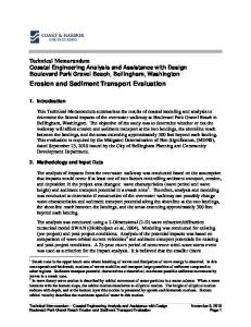
INTRODUCTION Montedoglio lake is a man-made lake located in Tuscany near Santo Stefano town, in the province of Arezzo (Figure 1). It was designed by Professor Filippo Arredi in 1971 to create a water reservoir, to stoke the Arezzo’s waterworks and to produce hydroelectric power. The catchment area includes three main rivers, Tevere, Singerna and Tignana, and is about 275.8 km2. The projected reservoir volume was about 168*106

Vol. 14, Bund. B 2 m3, the volume of the embankment dam about 2.7*106 m3 and the available volume of regulation about 142.5*106 m3, but no analysis was made of the possible quantity of sediment that could of deposited in the lake due to the detrital and colloidal rubbish carried downstream by the water.

Figure 1: The Map of Tevere river basin in Tuscany We have therefore analyzed the Montedoglio catchment by using a erosion-sedimentation model that values the moving processes of the erodible volume through the time. First of all, we analysed the erosive processes on that part of Tevere catchment by using RUSLE equation 1

A = R ⋅ K ⋅ L ⋅ S ⋅ C ⋅ P (ton/ha year) where o

A is the average annual soil loss in tons per hectare per year (ton/ha anno);

o

R is the rainfall/runoff erosivity and is calculated by summing the product of the storm kinetic energy times the maximum 30-min intensity for each storm occurring in an “n” year period as depicted in

R = E ⋅ I 30

((MJ mm)/(ha hour year))

in which the storm kinetic Energy E, function of the rainfall quantity and intensity I (mm·h-1), is calculated by summing the kinetic Energy ε (Mj·ha-1) of each interval having constant rainfall intensity as depicted in

ε = 0,119 + 0,0873 log I ε = 0,283 o

I ≤ 76 mm/h

I > 76 mm/h

K is the soil erodibility (t·ha-1·MJ-1·mm-1·ha·h) and is calculated by

[

]

K = 17.02 2.1⋅ 10 −4 M 1.14 (12 − a ) + 3.25(b − 2) + 2.5(c − 3) 100 in which M is calculated by M = α (100 − γ ) , function of the particle-size distribution (α is the silt ratio and γ the clay ratio), a is the organic-matter content, b the texture and c the permeability of the soil 12;

Vol. 14, Bund. B 3 o K is the hillslope length and is an expression of the effect of topography, specifically hillslope length, on rates of soil loss at a particular site. It is calculated by

L = ( λ 22.13)

m

λ is the hillslope length (m), 22.13 is the standard cell length and m is the exponent calculated by m = β (1 + β ) , in which β is function of the angle between the hillslope and the horizontal as depicted in β=

o

(sin θ 0.0896) . [ 3(sin θ ) 0.8 + 0.56]

S is the hillslope steepness and is an expression of the effect of hillslope steepness on rates of soil loss at a particular site. It is calculated by S = 10.8 sin θ + 0.03

s < 9% , λ > 15 ft (4.6 m)

S = 16.8 sin θ − 0.50

s ≥ 9% , λ > 15 ft (4.6 m)

S = 3(sin θ )

0.8

+ 0.56

λ < 15 ft (4.6 m)

where s is the hillslope steepness ratio. o

The C factor is an expression of the effects of surface covers and roughness, soil biomass, and soildisturbing activities on rates of soil loss at a particular site. C is calculated by specific schedules 1.

o

The P factor is an expression of the effects of supporting conservation practices, such as contouring, buffer strips of close-growing vegetation, and terracing, on soil loss at a particular site. If the hillslope is natural, not man-made and out of forestry, and has an high steepness, it’s used to take a unitary P factor as safety measure.

MATERIALS AND PROCEDURES FOR RUSLE CALCULATION To implement RUSLE equation we elaborated a Fortran program 2 that, dividing the catchment into cells having the same size of the DEM, allows to obtain for each cell the loss soil quantity (kg/year). The nine input data, in ASCII format, are as follows: the distributive map of the R factor (“pioggia.asc”), the distributive map of silt ratio in the soil (“alfa_bacino.asc”), the distributive map of clay ratio in the soil (“gamma_bacino.asc”), the distributive map of organic substance ratio in the soil (“a_bacino.asc”), the distributive map of texture class (“b_bacino.asc”), the distributive map of permeability class (“c_bacino.asc”), the distributive map of the steepness (degree) of the ground (“pendenze_gradi.asc”), the distributive map of C factor (“copertura.asc”) and the distributive map of cell size (“dominio.asc”). Before creating input ASCII data, we drew the boundary of the catchment area (275.8 km2) on the IGM topographic map of Tuscany (1:25000) geo-referenced in WGS84 coordinates (Figure 2) by using “computer-aided design” (CAD) software.

Vol. 14, Bund. B

4

Figure 2: The IGM Topographic map of Tuscany

Figure 3: The weather station in the analyzed Tevere catchment.

R Factor: input file To compute this factor we have firstly obtained the recording-gage precipitation records from each weather station in the catchment area (La Verna-Ar, Pieve Santo Stefano-Ar, Montedoglio-Ar, VergheretoFc, Monte Coronaro-Fc) (Figure 3). Following this, for each pluviometer, we identified all the storms occurring every year 3 and we calculated the respective annual R factor by summing the product of the storm kinetic energy times the maximum 30-min intensity for each storm occurring. We therefore estimated the average annual rainfall erosivity R by averaging all the annual R value for each weather station (Table 1) as depicted in

Vol. 14, Bund. B

5

R=

1  (E )k (I 30 )k     n j =1  k =1  n

m

where E is the total storm kinetic energy, I30 the maximum 30-min rainfall intensity, j the index of number of years used to produce the average, k the index of number of storms in a year, n the number of years used to obtain average R, m the number of storms in each year. Before calculating the ASCII file, we localised the pluviometers on the DWG file of the IGM topographic map by using CAD software and we drew the respective Thiessen polygons by using the GIS “CreateThiessenPoly” function, saving then the file as “shape”. Assigning every average annual R value to the respective polygon in the “shape” file and then converting the “shape” file in a raster file with a cell size of 20 metres, we obtained the file as shown in figure 4, in which the catchment is divided in parts with a specific R value. Finally, we converted the raster file in the respective ASCII file by using the “Raster to ASCII” GIS function, obtaining the file “pioggia.asc”.

Figure 4: The distributive raster map of the R factor

Table 1: The average annual rainfall erosivity for each weather station of the analysed catchment.

Weather Station

Average annual rainfall erosivity ((MJ mm)/(ha hour year))

La Verna Pieve Santo Stefano Montedoglio Verghereto Monte Coronaro

387,97 207,34 223,76 446,78 446,78

K Factor: input files To estimate the distributive maps of α, γ, a, b, c parameters, linked to K factor, we analysed the pedologic study about Tuscany soils (L. Gardin) 4. The Tevere catchment with the downstream section at

Vol. 14, Bund. B 6 Montedoglio has two main pedologic system: the “Alpe della Luna e rilievi intorno a Sestino” system and the “Pratomagno e Alpe di Catenaia” system.

“Alpe della Luna e rilievi intorno a Sestino” system This system is typified by a mountainous and hilly morphology, where the main lithologic facies are the “arenaceous calcareous flysch” (23%), “marly limes” (17%), “calcareous marly flysch” e “marl” (18%), “sandy flysch” (16%) and “argillite” (13%) (Figure 5). The pedoclimate is typified by a “udic” and “ustic” humidity regime and by a “mesic” temperature regime. The pedologic system is composed by 7 main cartographic units 9. The CTV1_SAL1_CLI1 cartographic unit (Lithology: quartzo-feldespatic sandstone, sometimes turbiditic, with intercalations of marls and argillites) includes soils developed on the “MarlySandy” facies and involves about the 30% of the system. The MNT1_GIU1_GSP1 unit (Lithology: siltic schist, marls, argillites and sandstone, usually turbiditic) includes the facies developed on Mugello rocks and involves about the 22% of the system. In both units, we find either erosive processes with different intensity or humidification and illuviation processes. The PGL1_TPG1_LBD1 unit (25% of the system) (Lithology: a chaotic argillaceous structure of marly limestone, ofiolitic gravels, calcarenites and limestone) is mainly composed by facies of argillites that have erosion and gleization processes. The VLB1_CLV1_PRT1 unit (19% of the system) (Lithology: white marly limestone with conchoidal fractures, slates and calcareous sandstone) is composed by facies originated on “marly calcareous flysch”, called “Alberese”, and is typified by either strong erosive processes or humidification and illuviation processes too. In this pedologic system the minor cartographic units are CPT1_CLO1_COC1(2%) and MPT1_COT1_MCR1 (2%). The first unit has a lithology composed by recent alluvions and without significant pedogenetic processes, the second a lithology of “Alberese” gravel diabases.

Figure 5: The map of the “Alpe della Luna” system

“Pratomagno e Alpe di Catenaia” system This pedologic system is typified by a mountainous and hilly morphology, having as main lithologic facies the “arenaceous flysch” (64%) and the “sandy argillaceous flysch” (20%), and by a pedoclimate having an “udic” and “ustic” humidity regime and a “mesic” temperature regime (Figure 6). The more common soils of the system have developed on “sandy flysch” and they belong to the MNT1_GIU1_GSP1

Vol. 14, Bund. B 7 unit (42%), the PON1_MRS1_PGG1 unit (32%) (Lithology: quartzo-feldespatic sandstone, sometimes turbiditic, with intercalations of marls and argillites), the SPV1_MCE1_LIP1 unit (9%) and the GRT1_PEL1 unit (8%). In this system we have firstly erosive processes and secondly processes of humidification, illuviation and brunification. The “arenaceous calcareous flysch” and “argillous scists” are in the VLB1_CLV1_PRT1 (5%) and PGL1_TPG1_LBD1 (4%) units, where we can observe strong erosive processes, and secondly, glaciation processes.

Figure 6: The map of the “Protomagno” system.

Physic and chemical characteristics of the cartographic units After analysing the main physic and chemical characteristics of the soils 10 in the cartographic units, we have obtained for each unit the elements needed to determine the α, γ, a, b, c parameters, as depicted in the following table (Table 2). Table 2: The physic and chemical characteristics for each cartographic units of the analysed catchment. Cartographic Unit

% Sand

% Clay

% Silt

% Organic Substance

USDA Texture class

CTV1_SAL1_CLI1 MNT1_GIU1_GSP1 PGL1_TPG1_LBD1 VLB1_CLV1_PRT1 CPT1_CLO1_COC1 MPT1_COT1_MCR1 PON1_MRS1_PGG1

30.2 29.9 18.9 26.5 42.4 47 56.4

22.2 21.3 38 26.5 22.5 18.8 13.8

60 30 50 20 30 30 20

2.18 2.57 2.57 2.81 2.12 3.13 2.9

FL F FLA FA F F FS

These values are, on average, weighted in the first 50cm of pedologic profiles linked to the same class of soils (STS) that have similar characteristics and behaviour. The arithmetic mean is weighted in proportion to the frequency of STS in the cartographic units (very frequent, frequent, little frequent, occasional) 4. According to the pedologic studies 4, 9, 10, 11, we have awarded the different RUSLE values of permeability and texture class to each USDA class of soil that we have in the catchment (Table 3).

Vol. 14, Bund. B

8

Table 3: The permeability and texture classes used in RUSLE calculation. USDA Class

RUSLE Permeability class

RUSLE Texture class

F FL FLA FS FA

Good (2) Good (2) Fair (3) Good (2) Good (2)

Fine texture (2) Fine texture (2) Fine texture (2) Middle texture (3) Middle texture (3)

Calculation of the inputs

Figure 7: Part of the Tuscan map of USDA texture class and the respective texture zones of the catchment area Firstly, on the Tuscan map of USDA texture class 4 georeferenced in WGS84 coordinates, we drew the boundary of the catchment area and we bounded together the different texture zones as closed polylines, as shown in figure 7. We opened this CAD file by using GIS software and then saved as a “shape” file, assigning every RUSLE value of texture class to the respective closed polyline. We converted the “shape” file into a “raster” file with a cell size of 20 metres by using a “Shape to raster” GIS function. Finally, we have converted the raster file in the respective ASCII file by using the “Raster to ASCII” GIS function, obtaining the file “b_bacino.asc”. Using the same input map and the same algorithms, we created the ASCII files of permeability and silt ratio, called respectively “c_bacino.asc” and “alfa_bacino.asc” respectively. In particular, in “c_bacino.asc” we assigned every RUSLE value of permeability class to the respective closed polylines and in “alfa_bacino.asc” every value of silt ratio, corresponding to the USDA classes, to the respective polylines. Moreover, to calculate the “gamma_bacino.asc” and “a_bacino.asc” input files, we have used the same proceedings of the previous input files but instead considered the Tuscan map of clay ratio 4 for the first file, and the Tuscan map of organic substance ratio for the second to bound the different zones.

L and S Factors: input file To calculate the “pendenze_gradi.asc” file needed for “L” and “S” RUSLE factors, we have firstly acquired the Digital Elevation Model of Tuscany that having a cell resolution of 20 metres. The DEM expresses each cell value of elevation expressed as metres on sea level, but the Fortran program needs cell values of hillslope expressed as degrees. We therefore re-sampled the DEM by using the “Analysis_Slope” GIS function, obtaining a “raster” with the slopes of the cells as degrees (figure 8). Finally, we converted the raster file in the respective ASCII file, obtaining “pendenze_gradi.asc”.

Vol. 14, Bund. B

9

Figure 8: Slope map of the analyzed catchment

Figure 9: Cover map for the analyzed catchment.

C Factor: input file The “copertura.asc” file relates to the effect of plants, soil covers, soil biomass and soil-disturbing activities on soil loss. Each cell values is computed by using the “shape” files of “Corine Land Cover” for the Tuscany, Marche and Emilia-Romagna regions 5. We opened these files by way of GIS software to associate in the “Open attribute table” of the “shape”, a C-RUSLE value to every different zone in according with the land use and the soil covers. The RUSLE values of C parameter are chosen by using the RUSLE experimental tables, 13 that show all the C values according to the different land use and the soil covers. Finally, we converted the new “shape” file in the respective raster file (figure 9) with a cell resolution of 20 metres and then in the corresponding ASCII file, obtaining the “copertura.asc” input file.

P factor: input file The “dominio.asc” input file helps the Fortran program to define the cell size, where it calculates the eroded soil, and the exact calculated catchment area. To create this ASCII file, we opened the DWG file of the catchment boundary by using GIS software, saving it as a “shape” file and then associating in the “Open attribute table” of the “shape” a unitary value to every cell. In this way, converting firstly the “shape” in the corresponding “raster” with a cell resolution of 20 metres and then in the ASCII file, we obtained the last input file (“dominio.asc”). In addition, the Fortran program assumes this ASCII file also as an output PRUSLE factor because we have adopted a unitary P value for all the analyzed catchment in according with the natural hillslopes and the high steepness.

Vol. 14, Bund. B

10

Figure 10: Map of the average annual soil loss (kg/year).

Calculation of the potential erosion: experimental results Implementing the Fortran program by the previous input files, we obtained the output map files relative to the RUSLE factor (K,L,S,R) and the average annual soil loss in kilo per cell per year (figure 10). Analyzing the map of the soil loss, we observed that the areas with a higher value of soil erosion are frequently in the source areas and throughout the principal axis of the rivers. This is due to the limited soil covers and the lithologic characteristics of the grounds, that have clay deposits (ofiolitic outcrop) with strong gully-shaped processes. The soil erosion is lower in the boundary areas of the catchment due to the dense forests, stable grasses and dense bushes. In addition, we have analyzed the map of soil erosion dividing the cells on the basis of the eroded thickness. This established that 88% of the catchment area has an annual eroded thickness of less than 1 mm (low erosion), 9% between 1 mm and 3 mm (middle erosion) and 3% more than 3 mm (high erosion). Every cell therefore has a specific value of annual eroded thickness. Summing up all these cell values by the “SOMMA_MATRICE.exe” Fortran program, we established the total amount of soil eroded and moved every year in the catchment (potential erosion). This is equal to 1.3285740*109 kg per year corresponding to 1.328.574 tons per year.

Figure 11: Iso-ipsa lines for the lake’s area in 1975.

Vol. 14, Bund. B

11

Multi-temporal and Morphologic Analysis for the catchment area The first step of the multi-temporal analysis regarded the reconstruction of the depth of the lake before the building of the dam in August 1975. We have acquired the 1975 photogrammetric images of the lake’s area from the Tuscan official photographic archives of IGM (Military Geographic Institute). These shots were taken by a low-level flight realized by the Luigi Rossi Firm of Florence on August 1975, about 5 years before the beginning of the dam’s construction, and they have a scale equal to 1:13000. The isoipsa lines were drawn and processed by the air-photogrammetric restitution of images, using a digital stero-plotter. This allowed us to obtain geographic accuracy such as with the 1:2000 scale, committing an error of the order of decimetre. The lines are georeferenced in the Gauss-Boaga coordinate system (west zone) and have an equidistance of 2 metres (Figure 11). In addition, to exactly place the foot of the dam we considered the 1992 Regional Technical Map (CTR) of Tuscany which has a scale of 1:5000. In fact, in this map the dam is in practice and the level of the lake is about 360 metres above the sea level. The creation of the 1975 Digital Elevation Model with a cell size of one meter was done by the “Create Tin/Raster” GIS function. This imported the 1975 isoipsa lines which have an altitude of between 344 metres and 400 metres above the sea level, the first corresponding to the level of the foot and the second to the level of the top of the dam. The second step regarded the data processing of the bathymetry, done on march 2004 6 by using the “Gps-Map 178 sounder” (Garmin firm).

Figure 12: DEM of the lake’s area in March 2004 We firstly acquired and processed the bathymetric data, completing the bathymetric points by using the geostatistic GIS functions, called “GIS_ArcToolbox_Raster Interpolation_Kriging”. We also completed the respective experimental variograms, and then, starting from these points, we drew the bathymetric lines by way of the “Interpolate GRID-Spline” GIS function 6. The bathymetric map is a DWG file where the isoipsa lines are typified by different depths from the lake level, approximately 384 metres above sea level in March 2004. Using the bathymetric lines, we reproduced the morphology of the lake by way of the “Create Tin/Raster” GIS function, obtaining the 2004 Digital Elevation model of the depth with a cell size of one metre (figure 12). As a result, we were then able to calculate the difference in volume between the 2004 DEM and the 1975 DEM. The calculation procedure consists of uploading the two digital elevation models on GIS software and the boundary mask of the lake as a closed polygon with a level of 384 metres. This mask is used by the software to carry out the calculation inside the lake’s area and is selected by the “3D Analyst-Analysis Mask” GIS function. The difference was calculated by the “Spatial Analyst-Raster Calculator” GIS function, thus obtaining a new DEM (“Calculation”) that could be analyzed by “3D Analyst-Surface Analysis-Area and Volume” function. With the difference, we determined a volume of sediment deposited equal to 9.053.474,63 m3, comprehensive of the volume of the dam. Subtracting the volume of the dam equal to 2.700.000 m3, we obtained the net volume of sediment deposited in the lake between 1990 and 2004. This value is equal to 6.3*106 m3, corresponding to about 450.000 m3/year. The

Vol. 14, Bund. B 12 annual value of sedimentation is relatively low because, among other things, the 15% of the catchment is on slow landslides, 7, 8 that mop up rainfall as a sponge, consequently generating a low value of superficial sediments.

Average specific volume for the sedimented particles To determine the water content and the effective dry mass of the deposited sediments, we took eight soil test specimens in different parts of the boundary of the lake in December 2007 (figure 13), when a wide area of the depth was exposed. In fact, the level of the lake was about 376 metres above sea level. The test points have the following Gauss-Boaga coordinates: A=(1747810.8607;4834610.6373;380.00) B=(1747624.4106;4834105.9578;376.00) C=(1747368.24;4832893.7868;376.00) D=(1746411.2766;4831683.0296;377.00) E=(1746873.8132;4830689.3367;376.00) F=(1747559.8320;4831103.0140;376.00) G=(1748090.4121;484831764.2204;376.00) H=(1748093.0544;4832876.4517;377.00)

Figure 13: The test points along the lake’s boundary. The soil test specimen were taken by a cylindrical hollow punch with a volume equal to one litre 35 and the UNI procedure 36 specifies the laboratory determination of water content. The water content is the ratio of the mass of “free” water in a given mass of soil material to the mass of the “dry” solid soil particles. We packed the specimens in a glass containers, and then we weighted them before placing in the “BINDER APT.LINE series E/B 28” drying oven maintained at 105°C ± 5°C for about 24 h. We used a balance (OHAUS PR OH8001085 serie ADVENTURER) with an accuracy of ± 3 g because the specimens have a mass greater than 1000g 36. After 24 hours in the drying oven, we weighted again the containers with the test specimens. We therefore determined the water content by using the following equation:

w=

W1 − W2 ∗ 100 W 2 − Wc

Vol. 14, Bund. B where

13

w is the water content (%); W1 is the mass of container and moist test specimen (g); W2 is the mass of container and dried test specimen (g); Wc is the mass of container (g). The water content could be considered an indirect index of the stress path of the specimen and it gives good informations about the shearing strength of the soil. In fact, the water content increases with the decrease of the shearing strength and with the increase of the compressibility. In the following table we report all the masses determined for each specimen and the respective water content (Table 4). Table 4: The water content determined for each soil test specimen.

For each specimen we therefore calculated the specific weight “γd” per unit volume of dried soil as from the specific weight “γ” per moist unit volume and the water content, by using the following geotechnical equation 37:

γd =

γ 1+ w

The specific weight “γ” is calculated by the ratio of the mass of moist soil test specimen to the volume of the same specimen. We have considered that the volume of the moist soil specimens is equal to the volume of the container (one litre). In the following table, for each specimen we calculated the specific weights “γd” per unit volume of dried soil. Table 5: The specific weights determined for each soil test specimen and the respective average value

Averaging the values of “γd” determined for each specimen, we obtained the average specific weight of the dried soils that compose the depth of the lake, and it’s equal to γd=1,76 tons/m3 (Table 5). We therefore determined the effective annual mass Ws of the sediments in the lake by using the following geotechnical equation

Vol. 14, Bund. B

14

γd =

Ws V

where V is the total annual volume of the sedimented soil and equal to 450.000 m3 per year, determined by the bathymetric analysis. The annual mass of the sedimented soil is equal to 792.000 tons per year.

Sediment Delivery Ratio The soil loss estimation with RUSLE model gives a clear indication of the amount of sediments moved every year on the watershed (potential erosion), but it doesn’t consider that an eroded grain can be subjected to sedimentation-movement cycles, during its downstream path and until its definitive sedimentation in the lake. The erosion mathematical models cannot simulate either the gully shaped erosion nor the erosion in the channels, because they only value the amount of soil eroded every year in the catchment and not how much eroded soil really arrives at the lake. We therefore multiplied the average annual soil loss “A” with the sediment delivery ratio (SDR), which allowed us to quantify how much eroded soil really comes into the lake every year (net erosion) in accordance with the prefixed temporal scale (year to year, in this case) 14. The estimation of SDR could be done by either at basin scale or at hillslope scale 15.

S.D.R at basin scale: experimental results We can calculate the exact annual average value of SDR for Montedoglio’s catchment because we know by bathymetry the exact amount of sediments deposited in the lake (Sp= annual average effective soil loss in the catchment) and by RUSLE equation the theoretic quantity of sediments moved every year (St = annual average quantity of soil moved in the catchment). S .D .R . =

792000 Sp × 100 = × 100 ≅ 60 % St 1328574

Figure 14: Stream map for the Montedoglio basin. This value shows how much more than half-eroded soil arrives every year (≈ 60%) to the lake located in correspondence with the downstream section of the basin. It also shows how the remaining part sediments due to the variation of acclivity, the superficial roughness, the permeability, the presence of vegetation, etc.. So the sediment delivery ratio depends on factors such as the typology of erosion (interrill, rills, gullies), the characteristics of sediment delivery system, the characteristics of the catchment, the texture of eroded soil, the conditions of vegetal cover etc. 16, 17. To verify the good quality of the SDR value determinated, we have analyzed the influence of the total length of the channel system, the influence of the superficial characteristics, the influence of the slopes and the granulometric composition of eroded soil. Firstly, we have

Vol. 14, Bund. B 15 observed that the SDR value is directly proportionate with the branching of the channel system. In fact, the more the system is branched the more the density of drainage is high and the sediments easily arrive to the channels, or even to the downstream section. We have calculated the channel system and its length by using the GRASS v6.2 as software and the DEM of the catchment area as input file. As a first step, we converted the original DEM into a DEM without depressions (“DEM fill”) by using r.fill.dir command, that allowed us to create a continuous channel system. We then calculated by r.watershed command the drainage lines and the stream map, resulting in a total length of about 733.76 km (figure 14). We were then able to calculate the drainage density, a morphometric quantity obtained by the ratio between the total length of the channels in kilometres and the area of the catchment in kilometres2 , showing how the catchment is divided in valleys.

Figure 15: Hillslope map for the Montedoglio basin. The areas with an inclination higher than 30° are colored red.

Dd =

Lreticolo 733,76 = = 2,66km −1 275,8 Abacino

Analyzing the channel system obtained, we observed a good drainage density, typical of superficial lithologies with a low permeability, that doesn’t allow the formation of intermediate re-depositions areas 18. Secondly, we know 16 that the average acclivity of the basin proportionality increases with the increase of the hillslopes and the inclination of the channels. Consequently the transport of eroded soil is easier. Analyzing the hillslope map (figure 15), we can observe that the catchment has an high average slope (≈ 16°) and a not excessive areal extension (≈ 276 km2), a typical characteristic of mountainous catchments, thus advantaging the transport of the sediments. Finally, the SDR values increase when the content of clay increases in the running off solutions, composed of water and eroded soil, and it decreases when the size of the sediments increases in the water. We analyzed the lithologic map of the high part of the Tevere’s catchment 19 (figure 16). Due to the lithologic and hydrologic characteristics of the catchment, we only considered the fine fraction of the transported materials, omitting the behaviour of the more massive sediments. In fact, the bigger sediments, originating mostly from the erosion of the channels, demand high velocities of the running water, so much so that the most of the bigger sediments are subject to re-deposition in channel. This is in comparison to the fine sediments, eroded mostly in the mountain slope, which are inclined to remain in suspension and to come easily to the downstream section. However the transport of fine sediments is particularly complicated and difficult to study because the eroded sediment moves in the form of aggregates instead of primary particles, causing a preferential deposit of fine particles (in particular clay) as macroaggregate. We considered the possibility that the clay-sized particles move along the hillslopes and in the channels without aggregating and re-depositing, due to the higher than average inclination of the catchment and the small size of the eroded grains like in the ophiolitic facies (in pink and red on the lithologic map). In particular, the lithologic map of the clayey content 20 shows how this content is on average high in the soils

Vol. 14, Bund. B 16 of the catchment, thus confirming the goodness of the SDR value determined experimentally. After verifying the precise SDR value, we related it with the geomorphologic elements of the catchment, to better understand the behaviour of the eroded volume in space and in time. Indeed, US research has underlined the existence of a important potential correlations between the surface of the catchment and the average annual SDR value 21, and the high variability of SDR values at the same area, due to the influence of particular characteristics of the catchments. In particular, for some American soils 22, the American Society of Civil Engineers 23 determined a potential relationship between the area of the catchment and the SDR value, as depicted by SDR= k * (S)n

Figure 16: Lithologic map of the high part of Tevere’s catchment. where SDR value is dimensionless, S is the area of the catchment in km2, and k and n are two constant values. The previous equation allows us to directly compare the correlations determined for the American soils with the trend obtained by analyzing particular Italian catchments. Whilst the equations for the American and Soviet soils show the n value changing from -0.01 to -0.25, 15 catchments, with an area between 10 km2 and 232 km2 are monitored and analyzed in Sicily, obtaining a regressive line that has SDR values higher than American and Soviet values for basins lower than 50 km2 24, 25, 26 . The Sicilian coefficient n is equal to 0.6953 and it is due to the particular physical characteristics of the Sicilian rivers. In fact they are essentially torrential with an high suspended transport just during the flood events, that are able to erode the beds of the channels and transport all the sediments, including the eroded soil on the hillslope. With the basins having a small area and these torrential rivers, we therefore observed that the erosive contribution of the channels is significant if compared with the contribution of the slopes. In the Tuscan-Emilian Apennine, several catchments have been monitored and analysed in the last few years, such as Montedoglio’s basin in the heart of the Tuscan-Emilian Apennine. In particular, the Sieve’s catchment (FI) 27, the basin of the Stura river (Fi) 27 , the basin of the Ritortolo river (Fi) 27 and the basin of the Sillaro river (Fi) 17 were monitored about the performance of the soil loss, analysing obviously the sediment delivery ratios. We were then able to determine the potential correlation among the catchment areas and the respective average annual SDR by compiling the following table (Table 6).

Vol. 14, Bund. B Table 6: The values of the catchment areas in km2 and the percentage values of the respective average annual Sediment Delivery Ratio. River

Tuscan-Emilian Apennine Downstream section

17

S (KM2)

SDR (%)

Sieve (Fi)

Bilancino’s dam (Fi)

128

36

Tevere (Ar)

275.8

60

Sillaro (Fi)

Montedoglio’s dam (Ar) Watersmeet section with Reno river (Fi)

137.6

8

Stura (Fi)

Bilancino’s dam (Fi)

39.6

58

Ritortolo (Fi)

Bilancino’s dam (Fi)

6.72

60

For the Tuscan-Emilian Apennine we have found a correlative trend having a potential equation such as SDR= 86.055 * (S)-0.2072, where the exponent n, equal to 0.2072, is included between -0.01 and -0.25, that is the range found for the American soil. In particular the exponent is close to the n values determinated for the Texan soils (n=0,18) and the soils of the Iowa (n=0,1) (Figure 17). We observed how the correlative line of the Apennine zone has a trend similar to the trends of Blackland Praire (Texas) and Corn Watershed (Iowa) This is the soils of the Tuscan-Emilian Apennine have an high content of clay like the analyzed American soils and so the eroded particles of soil remain in suspension and they don’t deposit again. Analysing other information 28, we observed a good correlation between the average annual SDR and some slope indexes. The first slope index is the ratio between the altimetric rise “Dmax” of the catchment, that is the difference between the maximum altitude of the basin and the altitude of the downstream section, and the length “L” of the main channel, while the second index is between the altimetric rise and the average inclination “P” of the main river 17, 18, 27. Firstly, considering the morphometric analysis undertaken in the Sieve’s catchment, in the basin of the Stura river and in the basins of the Ritortolo and Sillaro rivers, we obtained the first correlative trend between the average annual SDR and the first respective slope index, as depicted in the following table (Table 7) and graph (Figure 18). 120

Appennino Tosco-Emiliano Sicilia

-0,6953

y = 537,1x

SDR (%)

100 80

Texas

60

BlackLand Prairie Texas Corn Watersheds W Iowa US Southeastern Piedmont US Russia

40 20

-0,2072

y = 86,055x 0 10

100

1000

S (Km2)

Figure 17: The trends of the relationship between the areas of the catchments and the respective SDR values for different world places.

Vol. 14, Bund. B

18

Table 7: The values of the slope indexes and the percentage values of the respective average annual Sediment Delivery Ratio. Tuscan-Emilian Apennine Downstream River section Watersmeet Sillaro section with Reno river (Fi) Bilancino’s dam Sieve

Montedoglio’s dam

Tevere

Dmax (km)

L P Dmax÷L (km) (%)

Dmax÷P

SDR (%)

0.918

34

2.7

0.027

0.34

8

1.424

21

2

0.068

0.712

36

1.057

25

2.8

0.042

0.3775

60

70 y = 515.27x + 11.454 R2 = 0.1606

60

SDR (%)

50 40 30 20 10 0 0

0.02

0.04

0.06

0.08

0.1

Rapporto Dmax/L

Figure 18: The trend of the relationship between the Dmax/L and the respective SDR values for the analysed Apennine sites. As a second step, we analyzed the ratio between the average annual SDR and the second respective slope index, obtaining the following trend (Figure 19). 70 y = 16.056x + 27.349 R2 = 0.0154

60

SDR (%)

50 40 30 20 10 0 0

0.2

0.4

0.6

0.8

1

Rapporto Dmax/P

Figure 19: The trend of the relationship between the Dmax/P and the respective SDR values for the analysed Apennine sites.

Vol. 14, Bund. B 19 We observed how the two correlations have the same trend. Due to the mountainous and torrential characteristics of all of the rivers, due to the higher than average value of inclination of the main channel and the high content of clay in the soils of the basins, the SDR value increases with the increase of the altimetric rise and of the average inclination of the river. Consequently, the sediment suspended is easily carried to the downstream section, significantly decreasing the possibility of re-deposition. This is physically acceptable because the probability of temporary storage on the hillslopes and in the channels decreases with the increase of the average inclination of the catchment and of the main channel.

S.D.R analysis at hillslope scale: experimental results The analysis of the average annual sediment delivery ratio is an concise interpretation of the sediment delivery processes at basin scale, allowing us to know only the total effective quantity of sediment that every year arrives to the downstream section of the catchment and not the punctual value of SDR. The sediment delivery processes along the hillslope could be modelled by using a distributed approach because the sediments are the product of the erosive processes that happen in distributed areas of the catchment. So, using this approach we can punctually obtain the SDR values 29, that change in the catchment due to the variability of, for example, the inclination of the ground, the distance of the eroded areas from the rivers, the pedologic characteristics of the soils etc. A number of algorithms are constructed to calculate the SDR at a distributed scale but they are extremely arduous and suffer from some grade of mathematical approximation. In fact these mathematical models, valuing the soil loss at parcel scale, require a spatial distribution of the alleviation processes, all of which depends upon the sediment transfer from the eroded zone to the rivers. The spatial distribution concerns a division of the catchment in areas, homogenous about morphologic characteristics and in which the different erosive factors are valued and aggregated in accordance with the chosen algorithm. So the distributed approach thus allows us to properly determine punctually the spatial variability of the SDR. Due to the varying behaviour of the catchment areas to produce and transport sediments, we have to consider and separately model the sediment delivery on the hillslopes and the channel sediment delivery in the rivers. In particular, analysing the Montedoglio catchment and considering an average annual scale of a long period (14 years), we can consider the marginal the channel alleviation on the sediment transport with regard to Playfair’s law 30, which tells us that the rivers transport all the eroded soils to the channel and the fluvial transport capacity isn’t a limiting factor of the sediment transport in the channels. Under this hypothesis, the variability of the sediment delivery processes in the catchment could be considered by dividing the catchment in morphologic units and calculating the SDRi per every unit 18. We can then value the probability that a grain, eroded in the morphologic unit, arrives to the nearest channel. Therefore the scheme adopted to study the alleviation of the sediment transport is Lagrangian, because the particles are followed from the source area to the channel, and sequential, because the connection is realized by the sequential morphologic units along the hydraulic course 31, 32, 33.

Figure 20: Scheme of the Heuristic approach This, thought, doesn’t consider the impedance, that the sediments confront going to downstream and is due to the soil roughness, the tortuousness of the flux lines, the soil covers and the pedologic characteristics

Vol. 14, Bund. B 20 etc. A heuristic approach was thus developed 27 to calculate, a priori, the SDR values and the exact sediment quantity that arrives every year to the downstream section, unifying the downstream and upstream approaches and considering the impedance (figure 20). This new approach was validated by way of mountain catchment of the Sieve river with the downstream section at Bilancino’s dam, in the heart of Tuscan-Emilian Apennine. We therefore verified the heuristic algorithm to calculate the punctual SDR, applying it in the Montedoglio catchment, in the Tuscan-Emilian Apennine but far from Bilancino about 200 kilometres. Firstly, we calculated the Ddn distance index, that indicates the downstream connectivity of the single unit in the hillslope and is calculated as the sum of the single distances di, constituting the shortest downstream path. The di distances are weighted with the inverse of the CiSi product. The C factor introduces the weight of the superficial characteristics and the decrease of C is proportional to the increase of the roughness and the tortuousness.

Figure 21: Raster of Ddn index Whereas the decrease of S factor is proportional to the decrease of the transport capacity. So the index is

Ddn =  i

di , where di is the ith distance in meters of the downstream path on the single cell unit, Ci is the Ci S i

C factor of the single cell along the downstream path, Si is the slope gradient of the single cell along the downstream path (m/m). In practice, we have calculated the Ddn index (figure 21) by using the “flowlength” GIS function, the flow direction raster and the distributive map of the C factor as input data. In particular the flow direction raster is created by using the “flowdirection” GIS function and the Digital Elevation Model of the catchment as the only input data, while the map of the C represents the “weight” during the calculation of the index. In a second step, we calculated the Dup index, depicted by Dup = C S A , where the C factor is the average C factor of the upstream contributing area regarding the considered morphologic unit, the S factor is the average slope gradient of the upstream contributing area regarding the considered morphologic unit (m/m) and A is the contributing upstream area (m2). The Dup index is the length index of the contributing catchment and allowed us to consider the effects of the downstream fluxes about the mobility of sediments eroded on the considered morphologic unit. The combination of the C and S upstream values with the length of the contributing area allows us to weight the hydraulic impedance generated by the superficial characteristics (C) and the power of the downstream flux (S). In practice, we calculated the Dup index by using the “flowaccumulation” GIS function, the flow direction raster and the distributive map of the C factor as input data, obtaining a raster of the cumulated flux on every cell. As third

Vol. 14, Bund. B 21 step, we calculated the connectivity index Ic, dimensionless and associable to every cell of the DEM, by using

 n di    D  CS I c = l o g10  dn  = l o g10  i i i  D  C S A   up        The connectivity increases with the decrease of the  Ddn  value, and is high when we have high values D   up  for Dup and low values for Ddn. We have low values of connectivity index (less than 1) for the areas that are highly critical, whit further high values (more than 2) for the forests and the crest area. In practice we punctually calculated the connectivity index by using the “raster calculator” GIS function, obtaining a map with logarithmic values (figure 22). The critical areas, susceptible to re-deposition and with a red colour in the map, have the values of Ic between 1 and -4, while the forests and the stable area are between 3 and 5.6.

Figure 22: Raster of Ic index

Figure 23: Raster of punctual SDR values

Vol. 14, Bund. B 22 We found a range of Ic values between −4 and +5.6. If this is compared to the Bilancino’s (−4 and +8), we observe a smaller range due to the lower average value of Dup, and the smaller length of the flux paths and so the smaller transport capacity of sediments to the channels. In fact in Bilancino’s catchment, we can see longer flux paths and a higher transport capacity and so a smaller probability to sediment than Montedoglio’s. This is reflected in a wilder range of Ic values. As a last step, we determined the punctual distribution of Sediment Delivery Ratio (SDR). The relationship between the Ic index and the SDR was developed by direct observations of SDR values in the critical areas of Bilancino’s catchment. Because the range of the SDR values is physically included between 0 and 1 and in the Sieve’s catchment it assumed values between 0.4 and 0.6, the following Boltzmann function with two horizontal asymptotes was assumed, thus27

SDR = sdr2 +

sdr1 − sdr2 1+ e

−

I c0 − I c K

SDR = sediment delivery ratio (range between [0.0 -1.0] ); sdr1 = maximum sediment delivery ratio (assumed equal to 1.0); sdr2 = minimum sediment delivery ratio (assumed equal to 0.01); Ic0= connectivity index with a SDR =(sdr1+sdr2)/2=0.505 (assumed equal to 0.5); K = decay factor (assumed equal to1.5); Ic = connectivity index. In practice, we calculated the raster of the punctual SDR values by using the “raster calculator” GIS function, obtaining a range of values between 0 and about 0.95 (Figure 23). In the map, the zones having a red colour correspond with an high potentiality to re-deposition. Most of the SDR values are between 0.2 and 0.4, assuming an average value of 0.28 (Figure 24). In this way, the application of the Boltzmann function to another Appennine’s catchment, like Montegoglio, doesn’t imply an high conceptual imprecision 22. In fact, the function was created and calibrated by direct measures of SDR between 0.4 and 0.6 in the Bilancino’s catchment and we have observed that in the Montedoglio’s catchment, the average annual SDR value included in the range of calibration is approximately 0.6. In addition, both catchments belong to the same chain of mountains, the Tuscan-Emilian Apennines. We can therefore consider admissible to use the Boltzmann function in Montedoglio’s catchment. Valuing the absolute and relative errors committed by using the function 34, the absolute error is Errabs=0.28-0.60=-0.32, while the relative error is Errrel=-0.32/-0.60=-0.53. We can arrive at the same result by multiplying in GIS software the raster of punctual SDR values with the raster of the average annual soil loss (A factor), thus obtaining the map of annual eroded soil that effectively arrives at the Montedoglio’s lake. The raster calculation thus created regards the multiplication of the following factor: Anet=Apotential*SDR=R*L*S*C*K*P*SDR We thus obtained a punctual raster of the net erosion, or better of the quantity of the eroded soil that effectively leaves the catchment. The map has cells with net erosion values between 0 and 86 tons/year and, converting it in the respective ASCII file and then summing by using the “somma_matrice.exe” Fortran function, we obtained an annual quantity of sediments equal to 321.558,5 tons per year. This is a theoretic value of the annual quantity of soil deposited in lake, but the exact value calculated from the bathymetry is about 792.000 tons per year. The relative error is about -0.6.

Vol. 14, Bund. B

23

Figure 24: Distribution of the number of the cells of the basin in relation with the SDR values.

CONCLUSIONS The principal conclusions of the study described in this paper are as follows: 1. Implementing the RUSLE equation, the total amount “A” of the soil eroded and moved every year in the catchment of Tevere river with the downstream section at Montedoglio (Ar) (potential erosion), is equal to 1.3285740×109 kg per year corresponding to 1 328 574 tons per year. The multi-temporal and morphologic analysis for this catchment area (bathymetric analysis) allowed us to determine the real value of the soil eroded and deposited every year in the lake, equal to 6.3*106 m3, corresponding to about 450 000 m3 per year. To obtain the effective dry mass of the real deposited sediments in the lake, we determined the average specific weight of the dried soils that compose the depth of the lake, equal to γd=1,76 tons/m3, by analysing in the geotechnical laboratory the water content of eight soil test specimens taken in the depth of the lake. Therefore the effective annual mass Ws of the sediments deposited in the lake is equal to 792 000 tons per year, that, if compared with the potential erosive value (RUSLE), provides the real annual Sediment Delivery Ratio at basin scale, equal to 0.6 2. To better understand the behaviour of the eroded volume in space and in time, we related the SDR value at basin scale with the geomorphologic elements of the catchment, in according with US researches that has underlined the existence of important potential correlations between the surface of the catchment and the average annual SDR value, and the high variability of SDR values at the same area, due to the influence of particular characteristics of the catchments. For the TuscanEmilian Apennine we have found a correlative trend that has a potential equation such as SDR= 86.055 * (S)-0.2072, where the exponent n, equal to 0.2072, is included between -0.01 and -0.25, that is the range found for the American soil. In particular the exponent is close to the n values determined for the Texan soils (n=0,18) and the soils of the Iowa (n=0,1), due to the high content of clay of the soils of the Tuscan-Emilian Apennine. 3. At hillslope scale, we verified the heuristic algorithm, developed and validated by IRPI-CNR (Fi) 27 for the Bilancino’s basin to calculate the punctual SDR, applying it in the Montedoglio catchment, that is in the Tuscan-Emilian Apennine but far from Bilancino about 200 kilometres. In the Montedoglio’s, the critical areas, susceptible to re-deposition, have the values of connectivity index “Ic” between 1 and -4, while the forests and the stable area are between 3 and 5.6. We found a range of Ic values between -4 and +5.6. Calculating the punctual SDR values by the Boltzmann function for Montedoglio’s basin, we obtained a range of values between 0 and about 0.95 , with an average

Vol. 14, Bund. B 24 value equal to 0.28 . Therefore the application of the Boltzmann function to the Montedoglio’s basin to calculate the annual average SDR value, generates an absolute error equal to Errabs=0.28-0.60=0.32, while the relative error is Errrel=-0.32/-0.60=-0.53. 4. Multiplying in GIS software the raster of punctual SDR values with the raster of the average annual soil loss (A factor), we obtained the theoretical map of annual eroded soil that effectively arrives at the Montedoglio’s lake. The map has cells with net erosion values between 0 and 86 tons/year and the total amount is about 321.558,5 tons per year, that if compared with the exact value calculated from the bathymetry (792.000 tons per year), provides a relative error of -0.6. Results of this research demonstrate that the application of these theoretical methodologies in the Montedoglio’s catchment to determine the punctual SDR and the quantity of sediment that arrives every year to the lake, provides a range of error between 0.5 and 0.6. Therefore many questions remain and substantial research must be done prior to practical application of these algorithms to the basin of the Tuscan-Emilian Apennine. The results of study described are afflicted by an inaccuracy due to the subjective assignation of the C values to every different cover zones. The individuation and identification of the cover typologies and the respective height are in progress so as to decrease the errors of assignation. Anyway the results obtained by RUSLE equation are acceptable if we analyse the pedologic map of the basin. In fact observing the lithologic map, a large part of the catchment, more than 50 %, is composed by clayey formation (“Alberese” landscape, “Ophiliotic” landscape, “Argille-Scagliose” landscape), causing that the eroded particles of these soils remain in suspension and they don’t deposit again. This is in according with the RUSLE results that value a quantity of soil deposited in the lake about 60 % of the total moved eroded particles. Important areas for additional research include: the exact evaluation of the “C” cover values, the monitoring of the deposited sediments and the calibration of the RUSLE method and the algorithm elaborated by IRPI-CNR for the Tuscan-Emilian Apennine.

ACKNOWLEDGMENTS The research was sponsored by Demetra s.p.a research center, located in Perugia, Italy, and by the “Servizio Politiche attive del Lavoro” section of the Umbria Region. The writers are especially grateful to the “Ente Irriguo Umbro-Toscano” and in particular to Eng. Cola for his role in supporting this research.

REFERENCES 1. Book Terrence, J. Toy and George R. Foster -“Guidelines for the Use of the Revised Universal Soil Loss Equation”; 2. Book Ciaburro, G. “Manuale di Fortran”; 3. Website “Direzione Generale delle Politiche Territoriali ed ambientali - Servizio Idrologico Regionale”-Regione Toscana http://www.idropisa.it/; 4. Website Gardin, L.-“Progetto Carta dei suoli Regione Toscana” -http://www.rete.toscana.it/; 5. Website “Rete del Sistema Informativo Nazionale Ambientale”-http://www.clc2000.sinanet.apat.it/; 6. Symposium Pelini, R- “ Realizzazione di un Sistema Integrato per Batimetrie”- Proceedings of the International Geological Congress- Florence, August 2004; 7. Journal Guzzetti,F.‘et al.’- “Distribution of landslides in the Upper Tiber river basin, Central Italy. Landslides”. Geomorphology, Vol. 96, 105–122.; 8. Journal Guzzetti, F.- “Regional Hydrological thresholds for landslides and flood in the Tiber river basin”. J. Envir.Geology Vol. 35, N. 2-3 / August, 1998;

Vol. 14, Bund. B 25 9. Website Gardin, L. and Vinci, A.-“Catalogo delle unità cartografiche della carta dei suoli della Toscana in scala 1:250000” (2001) http://www.rete.toscana.it/; 10. Website Gardin, L. and Vinci, A.-“Catalogo dei suoli della carta dei suoli della Toscana in scala 1:250000” (2001) http://www.rete.toscana.it/; 11. Website Gardin, L. ‘et al.’-“Guida alla descrizione dei suoli in campagna e alla definizione delle loro qualità” (2001) http://www.rete.toscana.it/; 12. Book Giordani, C. and Zanchi, C.-“Elementi di conservazione del suolo” Patron ed. (1995); 13. Book Bagarello, V. Ferro, V.-“Erosione e conservazione del suolo” McGraw-Hill (2006); 14. Journal Bazzoffi, P. -“Erosione sui versanti e conseguente sedimentazione in piccoli serbatoi artificiali. Nota III: validazione di alcuni modelli di previsione dell’erosione (U.S.L.E, Gavrilovich, P.S.I.A.C) per mezzo del confronto fra i valori stimati e quelli effettivamente misurati attraverso la sedimentazione negli invasi”. Annali dell’Istituto Sperimentale per lo Studio e la Difesa del Suolo, 15: 149-188” (1984); 15. Book Wischeier, W.H. and Smith, D.D.- 1978 “Predicting rainfall erosion losses- A guide for conservation planning”. In: Agriculture Handbook 537, U.S.D.A; 16. Book Bagarello, V. ‘et al.’- “Manual sampling and tank size effects on the calibration curve of plot sediment storage tanks”. Transactions of the ASAE (2004), Vol. 47(4), 1105-1112; 17. Symposium Vianello, G. and Pavanelli, D.- “Stima dell’erosione del bacino Montano del torrente Sillaro con l’applicazione del modello RUSLE e attraverso il monitoraggio del trasporto in sospensione”. Proceedings of the “2th Giornata di Studio “Il monitoraggio idrotorbidimetrico dei corsi d’acqua per la stima dei processi erosivi e il bilancio dei solidi sospesi”- Bologna 8th October 2004; 18. Symposium Blois, L. and Bazzurro, F.: “Gestione ittica dell’invaso di Montedoglio”- Proceedings of the “Riunione Estiva della Società Geologica Italiana (San Cassiano 16-18 settembre 1996); 19. Website E.Van Waveren – “Ecologia del paesaggio dell'Alta Valle del Tevere - dati di base integrati per la “land evaluation” ” -http://www.rete.toscana.it/; 20. Website Gardin, L.- “Progetto Carta dei suoli Regione Toscana” http://www.rete.toscana.it/ ; 21. Journal Maner, S.B. -1962: “Factor influencing sediment delivery ratios in the Blackland Prairie land resource area”, U.S. Department of agriculture, Soil Conservation Service, Forth Worth, Texas, U.S.A.; 22. Journal Williams, J.R., Berndt, H.D. -1972- “Sediment yield computed with universal equation”, Journal of the Hydraulic Division, Proceedings of the American Society of Civil Engineers, 98, HY 12, 2087-2098; 23. Journal ASCE (American Society of Civil Engineers)-1975-, “Sedimentation engineering”, Am. Soc.Civ. Eng., New York, N.Y., Manual and reports on engineering practice, 54; 24. Journal Di Stefano C., Ferro V., Giordano G., Minacapilli M.- 2003: “Calibrazione di un modello distribuito per la stima della produzione di sedimenti in bacini di media estensione”, Quaderni di Idronomia Montana, 22, 233-248;

Vol. 14, Bund. B 26 25. Symposium Di Stefano C. ‘et al.’- 2005: “ Stima della produzione di sedimenti in due bacini sperimentali di differente estensione”, Atti del convegno AIIA “L’Ingegneria agraria per lo sviluppo sostenibile nell’area mediterranea”, Catania, 27-30 giugno, Memoria 6011; 26. Journal Di Stefano C., Ferro V., Porto P.- 2005: “ Monitoraggio nella produzione di sedimenti e calibrazione di un modello distribuito in un piccolo bacino forestato”, rivista di ingegneria agraria, 1, 35-50; 27. Website Borselli L., Menduni G., Ungaro F.: “Studio della dinamica delle aree sorgenti primarie di sedimento nell’area pilota del bacino di Bilancino :Progetto BABI”-http://www.adbarno.it/; 28. Journal Walling D.E.-1988: “The sediment delivery problem”, Journal of Hydrolgy, 65, 209-237; 29. Journal Boyce R.C.- 1975: “Sediment routing with sediment-delivery ratios”, Present and Prospective Technology for Predicting Sediment Yield and Sources, USDA, ARS-S-40, 61-65; 30. Journal Richards K.-1993: “Sediment delivery and drainage network”, Channel Network Hydrology, New York, 221-254; 31. Journal Ferro V., Porto P.-2000: “Sediment delivery distributed (SEDD) model”, Journal of Hydrologic Engineering October; 411-422; 32. Journal Di Stefano C.,Ferro V., Porto P.-2000: “Length Slope Factors for applying the Revised Universal Soil Loss Equation at Basin Scale in Southern Italy”, J. agric. Engng Res. 75; 349-364; 33. Journal Sun Ge , Mc Nutty S. G.-1999: “Modelling soil erosion and transport on forest landscape” Southern Global Change Program USDA Forest Service; 189-198 pp.; 34. Book Lo Cascio C.-2008:“Fondamenti di analisi numerica” McGraw-Hill; 35. ASTM D2487-06; ASTM D2488-00; Raccomandazioni AGI 1977; 36. UNI CEN ISO/TS 17892-1:2005- Geotechnical investigation and testing - Laboratory testing of soil - Part 1:Determination of water content; 37. Book Lancellotta, R.: “Geotecnica”-Zanichelli (2004).

© 2009 ejge